Infinite Multiple Membership Relational Modeling for Complex Networks
Abstract
Learning latent structure in complex networks has become an important problem fueled by many types of networked data originating from practically all fields of science. In this paper, we propose a new non-parametric Bayesian multiple-membership latent feature model for networks. Contrary to existing multiple-membership models that scale quadratically in the number of vertices the proposed model scales linearly in the number of links admitting multiple-membership analysis in large scale networks. We demonstrate a connection between the single membership relational model and multiple membership models and show on “real” size benchmark network data that accounting for multiple memberships improves the learning of latent structure as measured by link prediction while explicitly accounting for multiple membership result in a more compact representation of the latent structure of networks.
1 Introduction
The analysis of complex networks has become an important challenge spurred by the many types of networked data arising in practically all fields of science. These networks are very different in nature ranging from biology networks such as protein interaction [18, 1] and the connectome of neuronal connectivity [19] to the analysis of interaction between large groups of agents in social and technology networks [14, 19, 9, 20]. Many of the networks exhibit a strong degree of structure; thus, learning this structure facilitates both the understanding of network dynamics, the identification of link density heterogeneities, as well as the prediction of “missing” links.
We will represent a network as a graph where is the set of vertices and is the set of observed links and non-links. Let denote a link (adjacency) matrix where the element if there is a link between vertex and , if there is not a link, and if the existence of a link is unobserved. Furthermore, let , , and denote the set of links, non-links, and unobserved links in the graph respectively.
Over the years, a multitude of methods for identifying latent structure in graphs have been proposed, most of which are based on grouping the vertices for the identification of homogeneous regions. Traditionally, this has been based on various community detection approaches where a community is defined as a densely connected subset of vertices that is sparsely linked to the remaining network [15, 17]. These structures have for instance been identified by splitting the graph using spectral approaches, analyzing flows, and through the analysis of the Hamiltonian. Modularity optimization [15] is a special case that measures the deviation of the fraction of links within communities from the expected fraction of such links based on their degree distribution [15, 17]. A drawback, however, for these types of analyses is that they are based on heuristics and do not correspond to an underlying generative process.
Probabilistic generative models: Recently, generative models for complex networks have been proposed where links are drawn according to conditionally independent Bernoulli densities, such that the probability of observing a link is given by ,
| (1) |
In the classical Erdős-Rényi random graph model, each link is included independently with equal probability ; however, more expressive models are needed in order to model complex latent structure of graphs. In the following, we focus on two related methods: latent class and latent feature models.
Latent class models: In latent class models, such as the stochastic block model [16], also denoted the relational model (rm), each vertex belongs to a class , and the probability, , of a link between and is determined by the class assignments and as . Here, denotes the probability of generating a link between a vertex in class and a vertex in class . Inference in latent class models involves determining the class assignments as well as the class link probabilities. Based on this, communities can be found as (groups of) classes with high internal and low external link probability.
In the model proposed by [7] (hw) the class link probability, , is specified by a within-class probability and a between-class probability , i.e .. Another intuitive representation, which we refer to as db, is to have a shared between-class probability but allow for individual within-class probabilities, i.e . Both of these representations are consistent with the notion of communities with high internal and low external link density, and restricting the number of interaction parameters can facilitate model interpretation compared to the general rm.
Based on the Dirichlet process, [9, 20] propose a non-parametric generalization of the stochastic block model with a potentially infinite number of classes denoted the infinite relational model (irm) and infinite hidden relational model respectively. The latter generalizing the stochastic block model to simultaneously model potential vertex attributes. Inference in irm jointly determines the number of latent classes as well as class assignments and class link probabilities. This approach readily generalizes to the hw and db parameterizations of .
Latent feature models: In latent feature models, the assumption that each vertex belongs to a single class is relaxed. Instead it is assumed that each vertex has an associated feature , and that probabilities of links are determined based on interactions between features. This generalizes the latent class models, which are the special case where the features are binary vectors with exactly one non-zero element.

Many latent feature models support the notion of discrete classes, but allow for mixed or multiple memberships (see Figure 1 for an illustration of a network with multiple class memberships). In the mixed membership stochastic block model (mmsb) [1] the vertices are allowed to have fractional class memberships. In binary matrix factorization [11] multiple memberships are explicitly modeled such that each vertex can be assigned to multiple clusters by an infinite latent feature model based on the Indian buffet process (ibp) [6]. [12] study this approach, for the specific case of a Bernoulli likelihood, Eq. (1), and extend the method to include additional side information as covariates in modeling the link probabilities. In their model, the probability of a link is specified by , where is a function with range such as a sigmoid, and are weights that affects the probability of generating a link between vertices in cluster and . The term accounts for bias as well as additional side-information. For example, if covariates are available for each vertex , [12] suggest including the term , where , , and are regression parameters, and is some possibly nonlinear function.
In general, the computational cost of the single membership clustering methods mentioned above scales linearly in the number of links in the graph. Unfortunately, existing multiple membership models [1, 11, 12] scale quadratically in the number of vertices, because they require explicit computations for all links and non-links. This renders existing multiple membership modeling approaches infeasible for large networks. Furthermore, determining the multiple membership assignments is a combinatorial challenge as the number of potential states grow as rather than in single membership models. In particular, standard Gibbs sampling approaches tend to get stuck in local suboptimal configurations where single assignment changes are not adequate for the identification of probable alternative configurations [11]. Consequently, there is both a need for computationally efficient models that scale linearly in the number of links as well as reliable inference schemes for modeling multiple memberships.
In this paper, we propose a new non-parametric Bayesian latent feature graph model, denoted the infinite multiple relational model (imrm), that addresses the challenges mentioned above. Specifically, the contributions in this paper are the following: i) We propose the imrm in which inference scales linearly in the number of links. ii) We propose a non-conjugate split-merge sampling procedure for parameter inference. iii) We demonstrate how the single membership irm model implicitly accounts for multiple memberships. iv) We compare existing non-parametric single membership models with our proposed multiple membership counterparts in learning latent structure of a variety of benchmark ”real” size networks and demonstrate that explicitly modeling multiple-membership results in more compact representations of latent structure.
2 Infinite multiple-membership relational model
Given a graph, assume that each vertex has an associated -dimensional binary latent feature vector, , with assignments. Consider vertex and : For all combinations of classes there is an associated probability, , of generating a link. We assume that each of these combinations of classes act independently to generate a link between and , such that the total probability, , of generating a link between and is given by
| (2) |
where is an optional term that can be used to account for noise or to include further side-information as discussed previously. Under this model, the features act as independent causes of links, and thus if a vertex gets an additional feature it will result in an increased probability of linking to other vertices. In contrast to the model proposed by [12], where negative weights leads to features that inhibit links, our model is more restricted. Although this might result in less power to explain data, we expect that it will be easier to interpret the features in our model because links are directly generated by individual features and not through complex interactions between features. This is analogous to non-negative matrix factorization that is known to form parts-based representation because it does not allow component cancellations [10]. If the latent features have only a single active element and , Eq. (2) reduces to , i.e., the proposed model directly generalizes the irm model; hence, we denote our model the infinite multiple-membership relational model (imrm).
The link probability model in Eq. (2) has a very attractive computational property. In many real data sets, the number of non-links far exceeds the number of links present in the network. To analyze large scale networks where this holds it is a great advantage to devise algorithms that scale computationally only with the number of links present. As we show in the following, our model has that property. Assuming for simplicity of presentation, we may write Eq. (2) more compactly as ,
where the elements of the matrix are . Inserting this in Eq. (1) we have
| (3) |
The exponent of the second term, which entails a sum over the possibly large set of non-links in the network, can be efficiently computed as
| (4) |
requiring only summation over links and “missing” links. Assuming that the graph is not dominated by “missing” links, the computation of Eq. (3) scales linearly in the number of graph links, . We presently consider latent binary features , but we note that the model scales linearly for any parameterizations of the latent feature vector , as long as which holds in general if is non-negative.
As in existing multiple membership models [11, 12] we will assume an unbounded number of latent features. We learn the effective number of features through the Indian buffet process (ibp) representation [6], which defines a distribution over unbounded binary matrices,
| (5) |
where is the number of vertices belonging to class and is the number of columns of equal to .
As a prior over the class link probabilities we choose independent Beta distributions,
| (6) |
This is a conjugate prior for the single membership models where the parameters and correspond to pseudo counts of links and non-links respectively between classes and .
2.1 Inference
In the following we present a method for inferring the parameters of the model: the infinite binary feature matrix and the link probabilities . In the latent class model when only a single feature is active for each vertex, the likelihood in Eq. (3) is conjugate to the Beta prior for . In that case, can be integrated away and a collapsed Gibbs sampling procedure for can be used [9]. This is not possible in the imrm; instead, we propose to sample using Hamiltonian Markov chain Monte Carlo (hmc), and using Gibbs sampling combined with split-merge moves.
HMC for class link probabilities: Hamiltonian Markov chain Monte Carlo (hmc) [5] is an auxiliary variable sampling procedure that utilizes the gradient of the log posterior to avoid the random walk behavior of other sampling methods such as Metropolis-Hastings. In the following we do not describe the details of the hmc algorithm, but only derive the required expressions for the gradient. To utilize hmc, the sampled variables must be unconstrained, but since is a probability we make the following change of variable from to , , . Using the change of variables theorem, the prior for the class link probabilities expressed in terms of is given by . With this, the relevant terms of the negative log posterior is given by
| (7) |
where does not depend on . From this, the required gradient can be computed,
| (8) |
Again, the possibly large sum over non-links in the second term can be computed efficiently as in Eq. (4).
Gibbs sampler for binary features: Following [6], a Gibbs sampler for the latent binary features can be derived. Consider sampling the th feature of vertex : If one or more other vertices also possess the feature, i.e., , the posterior marginal is given by
| (9) |
When evaluating the likelihood term, only the terms that depend on need be computed and the Gibbs sampler can be implemented efficiently by reusing computation and by up and down dating variables.
In addition to sampling existing features, new features should also be associated with . [6] suggest “…computing probabilities for a range of values of up to some reasonable upper bound…”; however, following [11] we take another approach and sample the new features by Metropolis-Hastings using the prior as proposal density. The values of corresponding to the new features are proposed from the prior in Eq. (6).
Split-merge move for binary features: A drawback of Gibbs sampling procedures is that only a single variable is updated at a time, which makes the sampler prone to get stuck in suboptimal configurations. As a remedy, bolder Metropolis Hasting moves can be considered in which multiple changes of assignments help exploring alternative high probability configurations. How these alternative configurations are proposed is crucial in order to attain reasonable acceptance rates. A popular approach is to split or merge existing classes as proposed in [8] for the Dirichlet process mixture model (dpmm). Split-merge sampling in the ibp has previously been discussed briefly by [11] and [12].
Inspired by the non-conjugate sequential allocation split-merge sampler for the dpmm [4], we propose the following procedure: Draw two non-zero elements of , and . If propose a split — otherwise propose to merge classes and into a joint cluster . Accept the proposal with the Metropolis-Hastings acceptance rate, . In case of a merge, we remove and assign all its vertices to , and we remove the corresponding row and column of (this proposal is deterministic and has probability one). For a split, we remove all vertices except from cluster and create a new cluster and assign to it. We then sample a new row and column for the new cluster as described below. Next we sequentially allocate [4] the remaining original members of to either or or both in a restricted Gibbs sampling sweep, and refine the allocation through additional restricted Gibbs scans [8].
The proposal density for is based on a random walk, , where
| (10) |
such that has mean and variance equal to the empirical variance, . We choose the mean of the random walk as such that the new class has a similar within and between class link probabilities as the original class, but such that the class link probability between the original and new cluster is similar to the remaining between class link probabilities. This choice is crucial, since it favors splitting classes into two classes that are no more related than the relation to the remaining classes.
3 Results
Based on the hw, db, and rm parametrization of , we compared our proposed imrm to the corresponding single-membership irm [9]. We evaluated the models on a range of synthetically generated as well as real world networks. We assessed model performance in terms of ability to predict held-out links and non-links. As performance measure we used the area under curve (auc) of the receiver operating characteristic (roc). We also computed the predictive log likelihood (not shown here) which gave similar results. For comparison, we included the performance of several standard non-parametric link prediction approaches based on the following scores,
where is the degree of vertex .
In all the analyses we removed of the links and an equivalent number of non-links for cross-validation. We analyzed a total of five random data splits and all of the analyses were based on 2500 sampling iterations initialized randomly with clusters. Each iteration was based on split-merge sampling using sequential allocation with restricted Gibbs scans followed by standard Gibbs sampling. Our implementation of the irm was based on collapsed Gibbs sampling (i.e. integrating out ) as proposed in [9] but we also included a conjugate single-membership split-merge step corresponding to the proposed non-conjugate split-merge sampler. The priors were chosen as , , and , which renders the priors practically non-informative.
Synthetic networks: We analyzed a total of six synthetic networks generated according to the hw, db and rm models based on the vertices having either one or two memberships to the underlying classes. For the single membership models we generated a total of groups each containing 100 vertices. For the hw generated network we set and while for the db generated network we used a within community densities ranging from 0.2 to 1 while . The rm generated network had same within community densities as the db network but included varying degrees of overlap between the communities. The multiple membership models denoted mhw, mdb and mrm were generated from the corresponding single membership models as (where denotes element-wise or and is a random permutation matrix with diagonal zero), such that each vertex belongs to two classes.
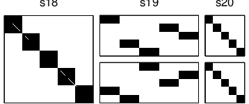
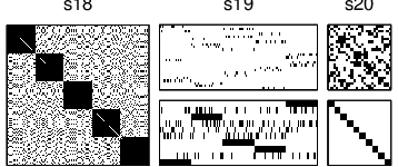


While the imrm model explicitly accounts for multiple memberships, the irm model can also implicitly account for multiple memberships through the between class interactions. To illustrate this, we analyzed the generated hw and mhw data by the irm model as well as the proposed imrm model (see Figure 2). When there are only single memberships, the imrm reduces to the irm model; however, when the network is generated such that the vertices have multiple memberships the imrm model correctly identifies the () underlying classes. The irm model on the other hand extracts a larger number of classes corresponding to all possible () combinations of classes present in the data. The estimated indicates how these classes combine to form the underlying multiple membership groups in the network. As such, the irm model has the same expressive power as the proposed multiple membership models but interpreting the results can be difficult when multiple membership community structure is split into several classes with complex patterns of interaction.
Figure 3 shows the link-prediction auc scores from the analysis of the six generated networks. Results show that all models work well on data generated according to their own model or models which they generalize. We also notice, that the irm model accounts well for multiple membership structure as discussed and illustrated in Figure 2. The hw and db models on the other hand fail in modeling networks with multiple memberships.
Real Networks: We finally analyzed five benchmark complex networks summarized in Table 1. The sizes of most of the networks makes it computationally infeasible for us to analyze them using the existing multiple-membership approaches proposed in [1, 11, 12]. For all the networks, multiple memberships are conceivable: In protein interaction networks such as the Yeast network proteins can be part of multiple functional groups, in social networks such as Erdos scientist collaborate with different groups of people depending on the research topic, and in word relation networks such as Reuters911 and FreeAssoc words can have multiple meanings/contexts. For all these networks explicitly modeling these multiple contexts can potentially improve on the structure identification over the equivalent single membership models.
| Network | Description | |||||
|---|---|---|---|---|---|---|
| Yeast | 2,284 | 6,646 | -0.10 | 0.13 | 4.4 | Protein-protein interaction network [18] |
| USPower | 4,941 | 6,594 | 0.00 | 0.08 | 19.9 | Topology of power grid [19] |
| Erdos | 5,534 | 8,472 | -0.04 | 0.08 | 3.9 | Erdös 02 collaboration network [2] |
| FreeAssoc | 10,299 | 61,677 | -0.07 | 0.12 | 3.9 | Word relations in free association [13] |
| Reuters911 | 13,314 | 148,038 | -0.11 | 0.37 | 3.1 | Word co-occurence [3] |
| ||||||||||||||||||
|
In Figure 4 the auc link prediction score is given for the five networks analyzed. As can be seen from the results, modeling multiple memberships significantly improves on predicting links in the network. In particular when considering the ihw and idb models and the corresponding proposed multiple membership models, the learning of structure is improved substantially for all networks except USPower. Furthermore, it can be seen that the irm model that can also implicitly account for multiple memberships in general has a similar performance to the multiple membership models. The poor identification of structure in the USPower network might be due to the fact that the average path between vertices are very high rendering it difficult to detect the underlying structure for any but the most simple ihw model. While the irm and imrm perform equally well in terms of link prediction it can be seen in table 2 that the average number of extracted components for the imrm model is significantly smaller than the number of components extracted by the irm model for all networks except the Reuters911 network where no significant difference is found. As a result, the imrm model is in general able to extract a more compact representation of the latent structure of networks. In table 2 is given the total cpu-time for estimating the 2500 samples for each of the network using the irm and imrm showing that the order of magnitude for the computational cost of the two models are the same.
4 Discussion
While single membership models based on the irm indirectly can account for multiple memberships as we have shown, the benefit of the proposed framework is that it allows for these multiple memberships to be modeled explicitly rather than through complex between-group interactions based on a multitude of single membership components. On synthetic and real data we demonstrated that explicitly modeling multiple-membership resulted in a more compact representation of the inherent structure in networks. We further demonstrated that models that can capture multiple memberships (which includes the irm model) significantly improve on the link prediction relative to models that can only account for single membership structure, i.e., the ihw and idb models. We presently considered undirected networks but we note that the proposed approach readily generalizes to directed and bi-partite graphs. Furthermore, the approach also extends to include side information as proposed in [12] as well as simultaneous modeling of vertex attributes [20]. We note however, that the inclusion of side information requires a linearly scalable parameterization in order for the overall model to remain computationally efficient. An attractive property of the irm model over the imrm model is that the irm model admits the use of collapsed Gibbs sampling which we have found to be more efficient relative to sampling the non-conjugate multiple membership models where additional sampling of the parameter is required. In future research, we envision combining the irm and imrm model, using the irm as initialization for the imrm or by forming hybrid models.
References
- [1] E. M. Airoldi, D. M. Blei, S. E. Fienberg, and E. P. Xing. Mixed membership stochastic blockmodels. J. Mach. Learn. Res., 9:1981–2014, 2008.
- [2] V. Batagelj and A. Mrvar. Pajek data sets, 2006.
- [3] S. R. Corman, T. Kuhn, R. D. McPhee, and D. K. J. Studying complex discursive systems: Centering resonance analysis of communication. Human communication research, 28(2):157–206, 2002.
- [4] D. B. Dahl. Sequentially-allocated merge-split sampler for conjugate and nonconjugate Dirichlet process mixture models. Technical report, Texas A&M University, 2005.
- [5] S. Duane, A. D. Kennedy, B. J. Pendleton, and D. Roweth. Hybrid monte carlo. Physics Letters B, 195(2):216–222, 1987.
- [6] T. L. Griffiths and Z. Ghahramani. Infinite latent feature models and the Indian buffet process. In Neural Information Processing Systems, Advances in (NIPS), pages 475–482, 2006.
- [7] J. M. Hofman and C. H. Wiggins. Bayesian approach to network modularity. Physical Review Letters, 100(25), Jun 2008.
- [8] S. Jain and R. M. Neal. A split-merge markov chain monte carlo procedure for the dirichlet process mixture model. Journal of Computational and Graphical Statistics, 13(1):158–182, 2004.
- [9] C. Kemp, J. B. Tenenbaum, T. L. Griffiths, T. Yamada, and N. Ueda. Learning systems of concepts with an infinite relational model. In Artificial Intelligence, Proceedings of the National AAAI Conference on, 2006.
- [10] D. D. Lee and H. S. Seung. Learning the parts of objects by non-negative matrix factorization. Nature, 401(6755):788–791, 1999.
- [11] E. Meeds, Z. Ghahramani, R. M. Neal, and S. T. Roweis. Modeling dyadic data with binary latent factors. In Advances in Neural Information Processing Systems (NIPS), volume 19, pages 977–984, 2007.
- [12] K. T. Miller, T. L. Griffiths, and M. I. Jordan. Nonparametric latent feature models for link prediction. In Advances in Neural Information Processing Systems (NIPS), pages 1276–1284, 2009.
- [13] D. L. Nelson, C. L. McEvoy, and T. A. Schreiber. The university of south florida word association, rhyme, and word fragment norms, 1998.
- [14] M. E. J. Newman. The structure of scientific collaboration networks. PNAS, 98(2):404–409, 2001.
- [15] M. E. J. Newman and M. Girvan. Finding and evaluating community structure in networks. Phys. Rev. E, 69(2):026113–1–15., 2004.
- [16] K. Nowicki and T. A. B. Snijders. Estimation and prediction for stochastic blockstructures. Journal of the American Statistical Association, 96(455):1077–1087, 2001.
- [17] J. Reichardt and S. Bornholdt. Statistical mechanics of community detection. Physical Review E, 74(1), 2006.
- [18] S. Sun, L. Ling, N. Zhang, G. Li, and R. Chen. Topological structure analysis of the protein-protein interaction network in budding yeast. Nucleic Acids Research, 31(9):2443–2450, 2003.
- [19] D. J. Watts and S. H. Strogatz. Collective dynamics of ’small-world’ networks. Nature, 393(6684):440–442, June 1998.
- [20] Z. Xu, V. Tresp, K Yu, and H.-P. Kriegel. Learning infinite hidden relational models. Uncertainity in Artificial Intelligence (UAI2006), 2006.