On Sharing Viral Video Over an Ad Hoc Wireless Network

In this paper we propose a simple and distributed file dissemination algorithm that takes advantage of two main ideas: (i) knowledge of the file spreads quickly because of the structure of the social network – we can use the same to manage file dissemination; (ii) in dense settings where ad hoc networks make sense, exploiting geographic proximity can provide additional benefits. With these ideas in mind, we devise a file dissemination algorithm that works by passing messages through the social network, and requires limited communication and computation overhead. In particular, the main features of our algorithm are as follows:

1. 1.

   Load balancing: users receiving a large amount of requests distribute them to nearby users on the social network, in such a way that we can guarantee no user has to serve more than six other users. Our algorithm achieves $\sqrt{n}$-scaling with the number of users receiving the file – sublinear, in sharp contrast to the linear scaling required in the WAN file dissemination architecture.

2. 2.

   Exploiting geographic proximity: We extend our load-balancing algorithm to exploit geographic proximity. Because of the structure of the social network, we show that by searching a few hops deeper in their social network, most users are able to download the file from another user at close range. This idea allows us to further reduce the scaling below $\sqrt{n}$, depending on the depth of the social-network a user may search.

3. 3.

   Social Networks: We analyze our algorithm on popular models for social networks (power law graphs). We show that the file dissemination time scales sublinearly with $n$ for a broad range of social-network parameters. In addition, we show that the performance of our algorithm is comparable to the best possible dissemination time of any algorithm – even those not constrained by communication or computation time.

Single piece file dissemination problems were first studied in [18][19]. In [20]-[22], they provide analytic results for multi-piece file dissemination problems. Other topics related to influence spreading, epidemics, and content distribution in social networks can be found, for example, in [23]-[25] and references therein.

Multi-hop transmission in a wireless network has been studied extensively since Gupta and Kumar’s seminal work [1]. Subsequently, [3] provides a simple proof and [2] closes the gap of $1/\sqrt{\log(n)}$. Multicast and broadcast capacities are considered in, e.g., [11]-[13]. On the other hand, [14]-[17] use randomized schemes to balance the traffic load and achieve throughput optimal routing.

We introduce the system model in Section II. In Section III, we present our algorithm and main results. Some lemmas regarding random placement and random graphs are included in Section IV. We analyze the performance of our algorithm in Section V. Conclusions are provided in Section VI. The proofs of various lemmas and theorems in Section III and Section IV can be found in Appendix A and Appendix B.

We model our network as $n$ static nodes, placed independently and uniformly on a square of width $\sqrt{n}$. Thus the (expected) density of the network stays constant. Each node has a transmitter and a receiver. All nodes can communicate with each other with fixed power $P$. The interference model is described by a Gaussian channel model defined below.

In this paper, we consider either $\gamma>0$ or $\gamma=0$ and $\alpha>2$.

As we identify users with their devices (e.g. cell phones/ PDA), the $n$ nodes in the wireless network also form a social network. A social network is described as a graph $G=(V,E)$ where $V$ is the set of nodes with cardinality $n$ and $E$ is the set of edges. Two nodes are joined by an edge if (and only if) the corresponding users are friends in the social network. The distance between two nodes $x$ and $y$ on the social-graph $G$ is the minimum number of hops between $x$ and $y$ in the social network. Thus a node’s neighbors are the nodes one hop away on the social graph, and its $k$-neighborhood are the nodes within $k$ hops away on the social graph. A key property we exploit is that distance between two nodes on the social network is generally unrelated to geographic distance between the corresponding users in the wireless network.

Empirical studies of many social (and other) networks have shown them to satisfy so-called power law graph structure, including many collaboration networks, but also the Internet and many communication networks (see e.g. [7] [8] [9] [10]). As a consequence, power law graphs (which we define below) are a popular choice for modeling social networks.

A graph $G$ is called a power law graph with parameter $\beta$ if the number of nodes with degree $k$ is proportional to $k^{-\beta}$. We will consider social networks generated by random power law graphs [4]. These random graphs satisfy an important property: each node has only small number of neighbors, i.e., small degree (small relative to the size of the overall network) while the diameter of the random graph (the maximum number of hops between the vast majority of the nodes) is still small, with overwhelming probability. This property is consistent with properties of most social networks, and in particular, with the famous observation known as the small world phenomenon, first discussed in [6].

As is common, we generate random graphs and in particular random power law graphs, according to expected degree sequences [4].

For convenience, we further introduce the following notation. Given a subset $S\subseteq V$, let the volume of $S$ be ${\rm vol}(S)=\sum_{i\in S}w_{i}$, $i.e.$, the sum of weights of nodes in $S$. Similarly, define ${\rm vol}_{k}(S)=\sum_{i\in S}w_{i}^{k}$ and $\tilde{d}={\rm vol}_{2}(G)/{\rm vol}(G)$.

The transmission time consists of two parts: propagation delay and file receiving time. The propagation delay is the time required to receive the first bit since the start of the transmission. The file receiving time is the time required to finish the transmission since then. For simplicity, we assume the file length $F$ is large, and we ignore the propagation delay in the analysis. We note in passing that we can formally incorporate both propagation delay as well as the file receiving time in our analysis by scaling $F$ such that the propagation delay terms will be sub-dominant to the file receiving time.

Our algorithm takes the input as the diameter of the social network, $D$, as well as two parameters which we specify: $\epsilon$, and $\mathcal{L}$, whose roles are as follows. Nodes are allowed to search for another node in the social network from which to download the file, at a distance of at most $2\epsilon D+1$ hops away. Thus if $\epsilon=0$, they cannot look beyond a single hop away, and if $\epsilon=0.5$, they have access to the entire social network. Thus the parameter $\epsilon$ controls the search depth. The parameter $\mathcal{L}$ is used to exploit geographic proximity: most nodes will download the file from nodes that are at a geographic distance of at most $\mathcal{L}$. If nodes have no notion of geography, we set $\mathcal{L}=\infty$, hence all nodes are within $\mathcal{L}$. Otherwise, we set $\mathcal{L}$ to a smaller value.

Given parameters $(\epsilon,\mathcal{L},D)$ as described above, the algorithm finds active nodes from which eager nodes can download the file. This is accomplished through coordination through the social network.

The main idea is the following: eager nodes send requests to one of their social-network neighbors with the file. Since a single node may get many such requests, it does not serve all of them, but rather finds other active nodes nearby in the social network to serve them, and also enlists the receiving nodes themselves to forward along the file. The theorems given in Sections III-B and III-C show that for the specific choices of parameters $\epsilon$ and $\mathcal{L}$ given, the algorithm succeeds in delivering the file to all nodes, and moreover does so in the advertised time scaling.

When $\mathcal{L}$ is set to a non-infinite value, it may not always be possible for nodes to obtain the file from geographically proximate neighbors – for instance, suppose the generator has no neighbors in her geographic proximity. In such cases, we allow file transfers that exceed geographic distance $\mathcal{L}$, and these happen from two or one-hop neighbors on the social network. We call transfers within geographic distance $\mathcal{L}$, $\mathcal{L}$-transfers, and all other transfers $S$-transfers, since they are near in the social-network distance. Similarly we refer to ${\mathcal{L}}$-requests and $S$-requests.

ALGORITHM 1:

Input: parameter $\epsilon$, distance threshold $\mathcal{L}$, and the diameter of the social network $D$.

Requesting Phase: Consider an eager node, $x$, at time $t$.

Step 1: Let $\mathcal{N}_{x}(t)$ denote node $x$’s $2\epsilon D+1$-neighborhood in the social-graph at time $t$. Let $\mathcal{N}_{x}^{\mathcal{L}}(t)\subseteq\mathcal{N}_{x}(t)$ be the set of nodes in $\mathcal{N}_{x}(t)$ that have the file and whose Euclidean (geographic) distance to $x$ does not exceed $\mathcal{L}$.

Step 2: If $\mathcal{N}_{x}^{\mathcal{L}}(t)$ is not empty, $x$ sends an ${\mathcal{L}}$-request to a randomly picked node in $\mathcal{N}_{x}^{\mathcal{L}}(t)$.

Step 3: If $\mathcal{N}_{x}^{\mathcal{L}}(t)$ is empty and the distance from $x$ to the source on the social-graph is smaller than $\epsilon D+1$, then $x$ sends an $S$-request to a one-hop neighbor in the social-graph which has the file.

Step 4: Otherwise, $x$ waits and goes back to step 1 at time $t+1$.

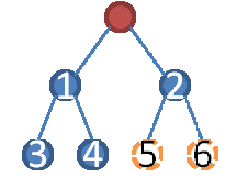
Scheduling Phase: Consider an active node $y$. It maintains two balanced binary trees, an $\mathcal{L}$-tree and an $S$-tree, constructed from its $\mathcal{L}$-requests and $S$-requests, respectively. It builds these trees by adding requesting nodes sequentially, as the requests arrive. This sequential building of the binary trees is depicted in Figure 1.

When node $y$ receives an $\mathcal{L}$-request, node $y$ adds the eager node to the $\mathcal{L}$-tree and asks its parent on the tree to deliver the file, and similarly for $S$-requests.

Transmission Phase: An eager node waits until the node designated as its transmitting node in the Scheduling Phase has the file. It then sets up a wireless transmission, and routes data through a highway system described in [2]. Note that the transmitter will have to serve at most 6 nodes: 2 from its own $\mathcal{L}$-tree, 2 from its own $S$-tree, and 2 from the tree it joins when it is an eager node (which could be either an $\mathcal{L}$-tree or an $S$-tree). Thus, we divide a time slot into six and each transmitter serves all nodes in a round robin fashion.

In this section we show that the load-balancing accomplished by the $\mathcal{L}$-binary trees is enough to give $\sqrt{n}$-scaling, without any geographic information. We show that our result holds, as long as the social network has the properties of a random power law graph with $\beta>2$, minimum expected degree $m>3$ and maximum expected degree $M$ satisfying $\log(n)\ll M\ll\sqrt{n}$ (many social networks have values of $\beta$ large than this – see, for example, collaboration graphs in [9]). In this case, the diameter of the social-graph is $\mathcal{O}(\log(n))$ and the size of the largest component is of $\Theta(n)$ [4][5].

As discussed, we set $\mathcal{L}=\infty$, and $\epsilon=0$, thus nodes are only allowed to request the file from nodes at most one hop away on the social network, and they entirely ignore geography.

In this case, for any eager node $x$, we have $\mathcal{N}_{x}^{\mathcal{L}}(t)\neq\emptyset$ at the time $t$ node $x$ becomes eager, and hence the Requesting Phase of the algorithm uses only Step 1 and Step 2. There are only $\mathcal{L}$-requests, and thus the algorithm requires each node to transmit to at most 4 other nodes. Indeed, the point of this algorithm is to distribute the load evenly on the wireless network.

In Theorem 4, we show that the file dissemination time scales like $\sqrt{n}$ (sublinearly). In addition, we show that the performance only differs from algorithm independent lower bounds with a factor $n^{\xi}$ for any $\xi>0$. Since the proofs of the following two theorems are similar to those for Theorem 7 and Theorem 8, we defer the full details to the Appendix B.

Intuitively, increasing the number of geographically proximal downloads should decrease transmission time. We show that this can be accomplished, at the cost of deeper searching of the social network, as long as the social network has the properties of a random power law graph with $\beta>3$ (again, many graphs have this property, see, e.g., the collaboration graphs in [10]). We assume that the minimum expected degree is $m=K\log(n)$ where $K$ is a constant greater than 10, and the maximum expected degree is $M$, satisfying $\log^{2}(n)\ll M\ll\sqrt{n}.$ Thus, almost all nodes are in the largest component and the diameter of the graph is $D\approx\log_{\tilde{d}}(n)$ [4][5] (recall the definition of $\tilde{d}$ from Section II).

Setting $\epsilon$ to a positive value translates to allowing nodes to search for an active node in their $2\epsilon\log_{\tilde{d}}(n)+1$-neighborhood, and because of our load-balancing architecture, ultimately download the file from nodes in their $4\epsilon\log_{\tilde{d}}(n)+2$ neighborhood. With more active nodes available, eager nodes can more easily find geographically proximal active nodes. We set $\mathcal{L}=8\sqrt{n^{1-\epsilon^{\prime}}\log(n)/\sigma\pi}$ for any $\epsilon^{\prime}<\epsilon$. The value of $\epsilon$ is chosen to be small, $\epsilon<1/10$, allowing nodes to search a neighborhood that is large, but nevertheless a vanishing fraction of the size of the entire network.

As load-balancing alone was able to achieve file dissemination time scaling of $\sqrt{n}$, we show now that by additionally exploiting geography, the file dissemination time can be further reduced by a factor $n^{\epsilon/2}$ compared to the result in Theorem 4. Proofs of the two theorems can be found in Section V.

Two properties in particular, are important. For our scheme to work, we need to show that with overwhelming probability, we will not have a very high clustering of nodes (some clustering will occur). We also need to show that when nodes look in their social network for geographically proximate active nodes, they will be able to find at least one, with high probability. The next two lemmas show precisely these properties.

In the first lemma, we show we control the minimum distance between a node and $k$ other nodes. We use this lemma to ensure that each node can find a node close to it on the wireless-square. In the second lemma, we show a concentration result about the number of nodes falling into a small rectangle, thus showing it is not too big. The proofs of these lemmas are also available in Appendix B.

In the following lemma, we address the relation between weights and the number of neighbors. Specifically, we show that if a node has weight $w_{i}$ greater than $10\log(n)$, then the number of one-hop neighbors the node can reach in the social-graph is between $w_{i}/2$ and $2w_{i}$. We use this lemma as it provides a relationship between weights and the number of nodes.

The next two lemmas characterize the local behavior of random power law graphs. Specifically, we are interested in how the size of neighborhoods of nodes in the largest component grows. We show that for any node in the largest component, the number of nodes in a small neighborhood grows like a factor $\tilde{d}$ if we explore one more step. We prove this by providing upper and lower bounds that only differ by a factor of $n^{\xi}$ for any $\xi>0$. The proofs are shown in Appendix A.

In this section, we first prove Theorem 7 which states the performance of our algorithm when geographic information is available, and when nodes can download the file from a neighborhood of radius $4\epsilon\log_{\tilde{d}}(n)+2$. The proof of the more simple load-balancing case (where we set $\mathcal{L}=\infty$ and $\epsilon=0$) is essentially a consequence of this proof – for the full details we refer to Appendix B. Specifically, we show the file dissemination time is roughly $\sqrt{n^{1-\epsilon}}F$.

The proof of the theorem consists of two main parts: showing the existence of a geographically nearby neighbor in the wireless-graph and the analysis of transmission rates. In addition, the transmission phase of our algorithm relies on some routing results from [2] and [12] which we summarize here. For the full details, we refer readers to those individual papers. In the routing scheme, packets are routed through a highway system consisting of horizontal highways and vertical highways. Each highway serves nodes in a stripe on the wireless-square. An illustration is shown in Fig. 2. The results in [2] and [12] guarantee the following properties of this highway system.

1. 1.

   Nodes can reach their highways in a hop of length $\mathcal{O}(\log(n))$.

2. 2.

   The highways are almost straight. For example, if a flow on a horizontal highway starts from $x$-coordinate $a_{1}$ with destination at $x$-coordination $a_{2}>a_{1}$, it will not reach any node with $x$-coordinate smaller than $a_{1}-H$ where $H=\mathcal{O}(\log(n))$.

3. 3.

   Highway nodes can communicate with neighboring highway nodes with a constant rate. A highway node serves flows through it with equal rate.

We now move to the proof of the theorem. We first state the existence of an “intermediate node” in the following lemma.

Thus, by Lemma 9, there exists a node $y$ among the $\sigma n^{\epsilon^{\prime}}$ nodes whose Euclidean distance to $x$ on the wireless-square is smaller than $\mathcal{L}$ with probability $1-o(n^{-1})$.  

Now, we bound the number of flows through a highway node at any time. Consider a transmission between two nodes with Euclidean distance less than $2\mathcal{L}.$ By the fact that highways are almost straight and the first and last hops are of length $\mathcal{O}(\log(n))$, the transmission passes through a horizontal (vertical) highway node only if the horizontal (vertical) distance between the transmitter (receiver) and the node is smaller than $3\mathcal{L}$ on the wireless-square. In other words, $\mathcal{L}$-transmissions through a horizontal (vertical) highway node must fall in a rectangle of side $6\mathcal{L}\times h$ in the corresponding horizontal (vertical) strip where $h$ is a constant provided in [2]. Since, by Lemma 10, the total number of nodes falling into this region is $\mathcal{O}(\mathcal{L})$ with probability $1-o(n^{-1})$ and each node generates at most a constant number of flows, using the union bound we can conclude that all highway nodes have at most $\mathcal{O}(\mathcal{L})$ $\mathcal{L}$-flows with probability $1-o(1)$. In addition, since there are at most $2Wn^{\epsilon^{\prime\prime}}/\log(n)$ $S$-transmissions, the total number of flows through each highway node is $\mathcal{O}(\mathcal{L})$ with probability $1-o(1)$. Therefore, each flow has a rate $\Omega(1/\mathcal{L})$ with high probability and each node can receive the file in $c_{0}\mathcal{L}F$ time slots for some constant $c_{0}>0$ from the time when the transmission begins.

We prove the theorem by induction on $k$: the distance from a node to the source on the social-graph. Let $\mathcal{N}_{k}$ denote nodes whose distance to the source is $k$ on the social-graph. The claim of the induction is that a node in $\mathcal{N}_{k}$ can receive the file in at most $kc_{0}\log_{2}(n)\mathcal{L}F$ time slots. By our notation, $\mathcal{N}_{0}$ is the source node. First note, that the base case $k=1$ of the induction clearly holds. Now, we suppose it is true for $k-1$ and consider nodes in $\mathcal{N}_{k}$. Note that no nodes in $\mathcal{N}_{k}$ are inactive at time $(k-1)c_{0}\log_{2}(n)\mathcal{L}F$. Further, by Algorithm 1 and Lemma 14, all nodes in $\mathcal{N}_{k}$ can request the file, according to the algorithm, from an active node in $\cup_{i=0}^{k-1}\mathcal{N}_{i}$. Thus, these nodes have to wait at most $\log_{2}(n)-1$ successful transmissions before starting to receive the file, since the depth of any binary tree is at most $\log_{2}(n)$. Therefore, they can receive the file before time $kc_{0}\log_{2}(n)\mathcal{L}F$. Hence, by induction, the file dissemination time is $\mathcal{O}(\sqrt{n^{1-\epsilon^{\prime}}}\log^{2.5}(n)F)$ as the diameter of the social-graph is $\mathcal{O}(\log(n))$.  

We proceed by first providing some definitions and a lemma. Given a transmission pair with rate $r$ over an Euclidean distance $\rho$ on the wireless-square, define the bit-meter rate of the transmission pair as $r\rho$. The total bit-meter product a network can transmit is the supremum of the sum of bit-meter products of all transmission pairs.

To prove the lower bound, we place no restrictions on computation or communication overhead. Moreover, we make (overly) optimistic assumptions throughout in order to guarantee a bound. For instance, we assume nodes only download from their nearest social-network neighbors.

Let $\mathcal{M}$ be the set of nodes in the largest component with expected degree in the range $[K\log(n)$ $2K\log(n)]$. Then,

since almost all nodes are in the largest component.

Fix any $\epsilon^{\prime}>\epsilon$. Let $\mathcal{N}_{i}$ be the set of nodes that node $i$ can reach in $4\epsilon\log_{\tilde{d}}(n)+2$ hops in the social-graph. Let $X_{i}$ be the indicator that the Euclidean distance from node $i$ to $\mathcal{N}_{i}$ on the wireless-square is smaller than $\sqrt{n/2\pi W\tilde{d}^{2}n^{4\epsilon^{\prime}}}$. Therefore, we have, for $i\in\mathcal{M}$ and $n$ large enough and some constant $c_{1}$,

since the probability that a node is close is smaller than $1/2W\tilde{d}^{2}n^{4\epsilon^{\prime}}$ and the second term comes from the probability that $|\mathcal{N}_{i}|\geq 2W\tilde{d}^{2}n^{4\epsilon^{\prime}}/\log(n)$. Therefore, we have

We claim that $\mathbb{P}(|\sum_{i\in\mathcal{M}}X_{i}-\mathbb{E}[\sum_{i\in\mathcal{M}}X_{i}]|\geq n/\log^{1/3}(n))=o(1).$ Indeed, by Chebyshev’s inequality, we have

where the last inequality follows from $\mathbb{E}[X_{i}X_{j}]\leq\mathbb{E}[X_{i}]$.

By the above claims, $|\mathcal{M}|=\Theta(n)$ while the number of nodes with geographically close neighbors in the wireless-square is $o(n)$. Hence, the transport load is $\Omega(n^{3/2-2\epsilon-\xi}F)$.  

We first quote lemma 3.2 from [4]. This useful lemma addresses how a neighborhood of a set in the random power law graph grows. Specifically, if we have two sets $S$ and $T$, what is the sum of weights of neighbors of $S$ which are also in $T$? One important application is the setting where $T\approx G$, i.e., $T$ is almost the entire graph. In this case, we get an increase factor of roughly $\tilde{d}$.

Using this lemma, we provide a proof to Lemma 12, which we used to lower bound the size of a node’s immediate neighborhood.

First notice that ${\rm vol}(S_{1})=\Omega(\log^{2}(n))$ with probability $1-o(n^{-1})$. This is true since, by Lemma 11, the node $x$ has at least $K\log(n)/2$ neighbors with probability $1-o(n^{-1})$ and each neighbor has weight at least $K\log(n)$.

We next verify (14) for $\beta>4$. Let $T_{i}$ be the set of all potential nodes whose distance to $x$ is $i+1$, i.e., $T_{i}=G\setminus\cup_{k=0}^{i}S_{k}$. Then, ${\rm vol}_{2}(T_{i})=(1+o(1)){\rm vol}_{2}(G)$ and ${\rm vol}_{3}(T_{i})=(1+o(1)){\rm vol}_{3}(G)$. Thus, $\frac{{\rm vol}_{3}(T_{i}){\rm vol}(G)}{{\rm vol}^{2}_{2}(T_{i})}=\Theta(1)$. Therefore, we have the result by induction.

For the case $3<\beta\leq 4$, let $T^{(k)}_{i}$ be the intersection of $T_{i}$ and the set of nodes with weight smaller than $k\log(n)$. Then, we have

and

Therefore, by (17), we have (15) is true by induction. On the other hand, ${\rm vol}_{2}(T_{i}^{(k)})/{\rm vol}(G)\approx\tilde{d}$ as $k$ becomes large enough, by (18).

With the above results, we can conclude that the size of the neighborhood grows by roughly a factor of $\tilde{d}/2$ with probability $1-o(n^{-2})$ for each step, from the second one to the $\epsilon\log_{\tilde{d}}(n)^{th}$ step. Since ${\rm vol}(S_{\epsilon\log_{\tilde{d}}(n)-1})\geq 2\sigma n^{\epsilon(1-o(1))}$ for some constant $\sigma$, there are at least $\sigma n^{\epsilon^{\prime}}$ nodes within distance $\epsilon\log_{\tilde{d}}(n)$ of $x$ in the social network.  

The proof of Lemma 13 depends on the following lemma from [5], that provides large deviation results for both an upper bound and a lower bound for the sum of Bernoulli random variables.

We now present the details of the proof. We first show the condition, ${\rm vol}(S_{0})\leq W$. Since $S_{0}=\{x\}$, we need to show the weight of $x$ does not exceed $W$ if $x$ is picked randomly.

where $C_{1}$ is the normalization constant $\int_{m}^{M}x^{-\beta}dx$. Thus, a randomly picked node $x$ has weight smaller than $W$ with high probability. Since by standard coupling arguments we see that the growth of the neighborhood of $x$ is dominated by a node with weight $W$, we simply take the weight of $x$ to be $W$ in what follows.

We turn to show ${\rm vol}(S_{i+1})\leq(1+\delta)\tilde{d}{\rm vol}(S_{i})$ with probability $1-\mathcal{O}(\log^{-2}(n))$. First, we give some definitions. Let $\tilde{m}_{i}=({\rm vol}(S_{i})\log^{\beta}(n))^{1/(\beta-2)}$ and define $T^{i}$ to be the set of nodes with weight greater than $\tilde{m}_{i}$. We first show that $T^{i}\cap S_{i+1}=\emptyset$ with probability $1-\mathcal{O}(\log^{-2}(n))$. Indeed,

where the first inequality follows from the union bound. Therefore, with high probability, $S_{i+1}\cap T^{i}=\emptyset$.

Define $\tilde{T}_{i}$ to be the set of unexplored nodes with weight smaller than $\tilde{m}$ in the $i$-th step, i.e., $\tilde{T}_{i}=V\setminus(T^{i}\cup\cup_{j=0}^{i}S_{j})$. Thus, $S_{i+1}$ is a subset of $\tilde{T}_{i}$. For simplicity, we consider a larger set $T_{i}$ which includes $\tilde{T}_{i}$ and virtual nodes $\tilde{V}_{i}$ where $\tilde{V}_{i}$ is chosen such that the number of nodes and their weights are the same as those in $\cup_{j=0}^{i}S_{j}$. We allow nodes in $S_{i}$ to connect to nodes in $\tilde{V}_{i}$ and, therefore, have a looser upperbound on ${\rm vol}(S_{i+1})$. We first give some properties of $T_{i}$. Specifically, we claim ${\rm vol}(T_{i})=(1+o(1)){\rm vol}(G)$ and ${\rm vol}_{2}(T_{i})=(1+o(1)){\rm vol}_{2}(G)$. Indeed,

where the inequality follows from ${\rm vol}(S_{i})$ will increase by a factor at least $\tilde{d}/2$ in each step as shown in Lemma 12. Similarly, we have ${\rm vol}_{2}(T_{i})=(1+o(1)){\rm vol}_{2}(G).$

Next, we give some properties of $S_{i+1}$. Our goal is to find the expected weight of $S_{i+1}$, $\mathbb{E}[Y_{i}]$, and the variable $\nu_{i}$ (defined below) to apply Lemma 17. To do this, define $X_{j}$ as the indicator function that node $j$ is in $S_{i+1}$. Thus, by union bound and a fact (in the proof of Lemma 3.2 in [4]), we have

Let $Y_{i}$ be the volume of $S_{i+1}$, i.e., $Y_{i}=\sum_{j\in T_{i}}w_{j}X_{j}$. Thus, we have

Similarly, define $\nu_{i}=\sum_{j\in T_{i}}w_{j}^{2}\mathbb{P}(X_{j}=1)$. We have

Using the properties of $T_{i}$ and $S_{i+1}$, we now show the inductive step, namely: ${\rm vol}(S_{i+1})\leq(1+\delta)\tilde{d}{\rm vol}(S_{i})$ with probability $1-o(\log^{-2}(n))$. Recalling Lemma 17, we have

References

- [1] P. Gupta and P. R. Kumar, “The capacity of wireless networks,” IEEE Transaction on Information Theory, Vol. 46, No. 2, pp. 388-404, 2000.
- [2] M. Franceschetti, O. Dousse, D. Tse, P. Thiran, “Closing the Gap in the Capacity of Wireless Networks Via Percolation Theory,” IEEE Transaction on Information Theory, Vol. 53, No. 3, pp. 1009-1018, 2007
- [3] S. R. Kulkarni and P. Viswanath, “A deterministic approach to throughput scaling in wireless networks,” IEEE Trans. on Information Theory, Vol. 52, No. 6, pp. 1041-1049, 2004.
- [4] F. Chung and L. Lu, “The average distances in random graphs with given expected degrees,” Internet Mathematics, Vol. 1, No. 1, pp. 91-114, 2002.
- [5] F. Chung and L. Lu, “Connected components in random graphs with given expected degree sequences,” Annals of Combinatorics, Vol. 6, pp. 125-145, 2002.
- [6] S. Milgram, “The small world problem,” Psychology Today, Vol 1, No. 1, pp. 60 ¡V 67, 1967.
- [7] R. Albert, H. Jeong, and A. Barabsi, “Diameter of the world wide web, Nature, pp. 130-131, 1999.
- [8] M. Faloutsos, P. Faloutsos, and C. Faloutsos, “On power-law relationships of the Internet topology,” ACM SIG-COMM, 1999.
- [9] A. L. Barabsi, H. Jeong, Z. Nda, E. Ravasz, A. Schubert, and T. Vicsek, “Evolution of the social network of scientific collaborations,” Physica A, Vol. 311, pp. 590-614, 2002.
- [10] J. Grossman, P. Ion, and R. De Castro, “Facts about Erds numbers and the collaboration graph,” available from the WWW: (http://www.oakland.edu/enp/trivia/), 2003.
- [11] X.-Y. Li, S.-J. Tang, and F. Ophir, “Multicast capacity for large scale wireless ad hoc networks,” ACM MobiCom 2007.
- [12] S. Li, Y. Liu, and X. -Y. Li, “Capacity of large scale wireless networks under gaussian channel model,” ACM MobiCom 2008.
- [13] S. Shakkottai, X. Liu, and R. Srikant, “The multicast capacity of ad hoc networks,” ACM MobiHoc 2007.
- [14] L. Tassiulas and A. Ephremides, “Stability properties of constrained queueing systems and scheduling for maximum throughput in multihop radio networks,” IEEE Trans. on Auto. Control, Vol. 37, no. 12, pp. 1936-1949, 1992.
- [15] P. Gupta and P. R. Kumar, “A system and traffic dependent adaptive routing algorithm for ad hoc networks,” Proc. IEEE 36th Conference on Decision and Control, 1997.
- [16] S. Subramanian, S. Shakkottai, and P. Gupta, “On optimal geographic routing in wireless networks with holes and non-uniform traffic,” Proc. IEEE INFOCOM 2007.
- [17] S. Subramanian, S. Shakkottai, and P. Gupta, “Optimal Geographic routing for wireless networks with near-arbitrary holes and traffic,” Proc. IEEE INFOCOM 2008.
- [18] A. Frieze and G. Grimmett, “The shortest path problem for graphs with random arc lengths,” Discrete Applied Mathematics, pp. 577, 1985.
- [19] B. Pittel, “On spreading a rumor,” SIAM Journal of Applied Mathematics, Vol. 47, No. 1, pp. 213-223, 1987.
- [20] R. Karp, C. Schindelhauer, S. Shenker, and B. Vcking, “Randomized rumor spreading,” Proceedings of the 41st Annual IEEE Symposium on Foundations of Computer Science, 2000, pp. 565-574.
- [21] S. Sanghavi, B. Hajek, and L. Massouli, “Gossiping with Multiple Messages,” IEEE Trans on Information Theory, Vol. 53, No. 12, pp 4640-4654, 2007
- [22] S. Deb and M. Mdard, “Algebraic gossip: A network coding approach to optimal multiple rumor mongering,” Proceedings of the 42nd Annual Allerton Conference on Communication, Control, and Computing, 2004.
- [23] D. Kempe, J. Kleinberg, and Tardos, “Maximizing the spread of influence through a social network,” ACM KDD, 2003.
- [24] A. Ganesh, L. Massouli, and D. Towsley, “The effect of network topology on the spread of epidemics,” IEEE INFOCOM, 2005.
- [25] S. Ioannidis, A. Chaintreau, and L. Massouli, “Optimal and Scalable Distribution of Content Updates over a Mobile Social Network,” IEEE INFOCOM, 2009.