跳到论文正文
W Papers独立论文阅读器 arXiv:1101.4714 论文正文 计算阅读时间 · 0%
引用这篇论文根据当前论文元数据生成,正式投稿前建议核对。


License: CC BY-NC-SA 3.0
arXiv:1101.4714v2 [hep-ph] 27 Oct 2011

Nonleptonic two-body decays of charmed mesons

Fu-Sheng Yu, Xiao-Xia Wang, and Cai-Dian Lü Affiliation: Institute of High Energy Physics and Theoretical Physics Center for Science Facilities, Chinese Academy of Sciences, Beijing 100049, People’s Republic of China
Abstract

Nonleptonic decays of charmed mesons into two pseudoscalar mesons or one pseudoscalar meson and one vector meson are studied on the basis of a generalized factorization method considering the resonance effects in the pole model for the annihilation contributions. Large strong phases between different topological diagrams are considered in this work, simply taking the phase in the coefficients aia_{i}. We find that the annihilation-type contributions calculated in the pole model are large in both of the P​PPP and P​VPV modes, which make our numerical results agree with the experimental data better than those previous calculations.

PACS: 13.25.Ft, 11.15.Tk, 11.30.Hv, 12.39.St

I Introduction

Nonleptonic decays of charmed mesons are very interesting as they can provide useful information on flavor mixing, CP violation, and strong interactions[1]. They may also shed light on any new physics signal through D0−D¯0D^{0}-\bar{D}^{0} mixing and rare decays[2, 3, 4, 5, 6, 7]. The CLEO-c and two B factories experiments have given many new results on this subject and more are expected soon from the BES-III experiment. Besides, theoretical studies have been in progress for decades.

With the heavy quark effective theory, many QCD-inspired approaches, such as the QCD factorization approach [8], the perturbative QCD approach [9], and the soft-collinear effective theory [10], successfully describe the hadronic B decays. However, this is not the case for the DD meson decays. These approaches do not work well here, due to the mass of charm quark, of order 1.5GeV, which is not heavy enough for a sensible heavy quark expansion, neither light enough to apply the chiral perturbation theory.

After decades of studies, the factorization approach is still one of the effective ways to deal with the two-body charmed meson decays[11]. However, it is well known that some difficulties exist in the naive factorization approach: the Wilson coefficients a1​(μ)a_{1}(\mu) and a2​(μ)a_{2}(\mu) of effective operators are renormalization scale and γ5\gamma_{5}-scheme dependent; and the color-suppressed processes are not calculated well due to the smallness of a2a_{2}, etc. In order to solve these problems, the so-called generalized factorization approach was proposed [12]. The Wilson coefficients a1​(μ)a_{1}(\mu) and a2​(μ)a_{2}(\mu) are not from direct calculation any more but are effective coefficients to accommodate the important nonfactorizable corrections [13]. In these naive or generalized factorization approaches, there is almost no strong phase. But large strong phases have been found from DD decay experiments. A corresponding large relative strong phase between the factorization coefficients a1a_{1} and a2a_{2} has been discussed in [14, 15].

Unsatisfied by the short comings of the factorization approach, the model-independent diagrammatic approach, with various topological amplitudes extracted from the data, is recently applied to two-body hadronic DD decays [16, 17, 18, 19]. They use SU(3) symmetry in their analysis to avoid model calculations. All the parameters are fitted from experiments to give a better agreement with the experimental data but with less predictive power. More precise predictions are limited in this approach due to the uncontrolled SU(3) breaking effect[15]. These analyses also show that large annihilation type contributions are needed to explain the data, which can not be calculated in the naive or generalized factorization approaches. The kind of pure annihilation type DD meson decays also needs to be systematically analyzed [20].

In another aspect, the hadronic picture description of nonleptonic weak decays has a longer history, because of their nonperturbative feature. Based on the idea of vector dominance, which is discussed on strange particle decays[21], the pole-dominance model of two-body nonleptonic decays is proposed [22]. Beyond the vector dominance pole, this model also involves scalar, pseudoscalar, and axial-vector poles. For simplicity, only the lowest-lying poles are considered. This model has already been applied to charmed meson and bottom meson decays [22, 23], where it is approved that this model is more or less equivalent to the factorization approach in the first order approximation.

In this work, we will use the generalized factorization approach but with a relative strong phase between the Wilson coefficients a1a_{1} and a2a_{2} to accommodate the nonfactorizable contributions. For the uncalculable annihilation type contributions, we use the pole model. In this case, we can really calculate most of the important contributions in the hadronic DD decays, which are demonstrated in the model-independent diagrammatic analysis [19].

The outline of this paper is as follows. In Sec.II, we give the formulas of this work, showing the generalized factorization approach and the pole-dominance model. In Sec.III, our results are given and compared to the experimental data and those of the diagrammatic approach and the calculations considering the final-state interaction of nearby resonances effects. Summary and conclusions are followed.

II Formalism

II.1 The factorization approach

First we begin with the weak effective Hamiltonian He​f​fH_{eff} for the Δ​C=1\Delta C=1 transition [24]:

ℋe​f​f=GF2​VC​K​M​(C1​O1+C2​O2)+h.c.,\mathcal{H}_{eff}=\frac{G_{F}}{\sqrt{2}}V_{CKM}(C_{1}O_{1}+C_{2}O_{2})+h.c., (1)

where VC​K​MV_{CKM} is the corresponding Cabibbo-Kobayashi- Maskawa (CKM) matrix elements, C1,2C_{1,2} are the Wilson coefficients. The current-current operators O1,2O_{1,2} are

O1=u¯α​γμ​(1−γ5)​q2​β⋅q¯3​β​γμ​(1−γ5)​cα,\displaystyle O_{1}=\bar{u}_{\alpha}\gamma_{\mu}(1-\gamma_{5})q_{2\beta}\cdot\bar{q}_{3\beta}\gamma^{\mu}(1-\gamma_{5})c_{\alpha},
O2=u¯α​γμ​(1−γ5)​q2​α⋅q¯3​β​γμ​(1−γ5)​cβ,\displaystyle O_{2}=\bar{u}_{\alpha}\gamma_{\mu}(1-\gamma_{5})q_{2\alpha}\cdot\bar{q}_{3\beta}\gamma^{\mu}(1-\gamma_{5})c_{\beta}, (2)

where α,β\alpha,\beta are color indices, and q2,3q_{2,3} are dd or ss quarks.

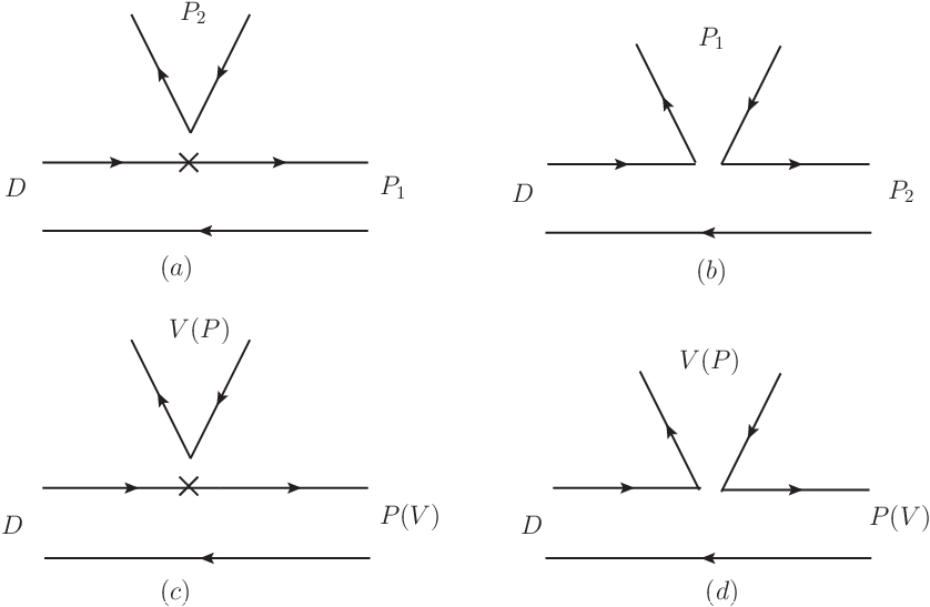
Refer to caption
Figure 1: Emission-type diagrams in the factorization approach.

The color-favored emission diagram corresponding to D→P​PD\to PP decays, with PP representing a pseudoscalar meson, is shown in Fig. 1 (a). Under the factorization hypothesis, the transition matrix element of hadronic two-body charmed meson decays is factorized into two parts [11]:

⟨P1​P2|ℋe​f​f|D⟩\displaystyle\langle P_{1}P_{2}|\mathcal{H}_{eff}|D\rangle =\displaystyle= GF2​VC​K​M​a1​⟨P2|u¯​γμ​(1−γ5)​q2|0⟩​⟨P1|q¯3​γμ​(1−γ5)​c|D⟩.\displaystyle\frac{G_{F}}{\sqrt{2}}V_{CKM}a_{1}\langle P_{2}|\bar{u}\gamma_{\mu}(1-\gamma_{5})q_{2}|0\rangle\langle P_{1}|\bar{q}_{3}\gamma^{\mu}(1-\gamma_{5})c|D\rangle. (3)

Similarly, the contribution of the color-suppressed diagram shown in Fig. 1 (b) is given as

⟨P1​P2|ℋe​f​f|D⟩\displaystyle\langle P_{1}P_{2}|\mathcal{H}_{eff}|D\rangle =\displaystyle= GF2​VC​K​M​a2​⟨P1|q¯3​γμ​(1−γ5)​q2|0⟩​⟨P2|u¯​γμ​(1−γ5)​c|D⟩,\displaystyle\frac{G_{F}}{\sqrt{2}}V_{CKM}a_{2}\langle P_{1}|\bar{q}_{3}\gamma_{\mu}(1-\gamma_{5})q_{2}|0\rangle\langle P_{2}|\bar{u}\gamma^{\mu}(1-\gamma_{5})c|D\rangle, (4)

where

a1​(μ)=C2​(μ)+C1​(μ)Nc,\displaystyle a_{1}(\mu)=C_{2}(\mu)+\frac{C_{1}(\mu)}{N_{c}}, a2​(μ)=C1​(μ)+C2​(μ)Nc,\displaystyle a_{2}(\mu)=C_{1}(\mu)+\frac{C_{2}(\mu)}{N_{c}}, (5)

correspond to the color-favored tree diagram (𝒯\mathcal{T}) and the color-suppressed diagram (𝒞\mathcal{C}) respectively in the naive factorization, with the number of colors Nc=3N_{c}=3. They are assumed to be universal and process-independent in the native factorization approach. The current matrix elements in Eqs.(3,4) are evaluated in terms of transition form factors and decay constants. For D→P​PD\to PP decays, the form factor is defined as follows:

⟨P⁡(k)|q¯3​γμ​(1−γ5)​c|D⁡(p)⟩\displaystyle\langle P(k)|\bar{q}_{3}\gamma_{\mu}(1-\gamma_{5})c|D(p)\rangle =\displaystyle= [(p+k)μ−mD2−mP2q2​qμ]​F1D→P​(q2)\displaystyle\bigg[(p+k)_{\mu}-\frac{m_{D}^{2}-m_{P}^{2}}{q^{2}}q_{\mu}\bigg]F_{1}^{D\to P}(q^{2}) (6)
+mD2−mP2q2​qμ​F0D→P​(q2),\displaystyle+\frac{m_{D}^{2}-m_{P}^{2}}{q^{2}}q_{\mu}F_{0}^{D\to P}(q^{2}),

where q=p−kq=p-k, and FiF_{i} are the corresponding transition form factors. The decay constants fPf_{P} of pseudoscalar mesons are defined as

⟨P⁡(q)|q¯1​γμ​(1−γ5)​q2|0⟩\displaystyle\langle P(q)|\bar{q}_{1}\gamma_{\mu}(1-\gamma_{5})q_{2}|0\rangle =\displaystyle= i​fP​qμ.\displaystyle if_{P}q_{\mu}. (7)

In terms of decay constant and transition form factors, the decay amplitude of Figs.1 (a) and (b) are then

⟨P1​P2|ℋe​f​f|D⟩T\displaystyle\langle P_{1}P_{2}|\mathcal{H}_{eff}|D\rangle_{T} =\displaystyle= i​GF2​VC​K​M​a1​fP2​(mD2−mP12)​F0D→P1​(mP22),\displaystyle i\frac{G_{F}}{\sqrt{2}}V_{CKM}a_{1}f_{P_{2}}(m_{D}^{2}-m_{P_{1}}^{2})F_{0}^{D\to P_{1}}(m_{P_{2}}^{2}), (8)
⟨P1​P2|ℋe​f​f|D⟩C\displaystyle\langle P_{1}P_{2}|\mathcal{H}_{eff}|D\rangle_{C} =\displaystyle= i​GF2​VC​K​M​a2​fP1​(mD2−mP22)​F0D→P2​(mP12).\displaystyle i\frac{G_{F}}{\sqrt{2}}V_{CKM}a_{2}f_{P_{1}}(m_{D}^{2}-m_{P_{2}}^{2})F_{0}^{D\to P_{2}}(m_{P_{1}}^{2}). (9)

The diagrams for D→P​VD\to PV decays, with VV denoting a vector meson, are shown in Figs. 1 (c) and (d). If the out-emitted particle is a pseudoscalar meson, the matrix element of Fig. 1 (c) is

⟨P​V​|ℋe​f​f|​D⟩\displaystyle\langle PV|\mathcal{H}_{eff}|D\rangle =\displaystyle= GF2​VC​K​M​a1​⟨P|u¯​γμ​(1−γ5)​q2|0⟩​⟨V|q¯3​γμ​(1−γ5)​c|D⟩.\displaystyle\frac{G_{F}}{\sqrt{2}}V_{CKM}a_{1}\langle P|\bar{u}\gamma_{\mu}(1-\gamma_{5})q_{2}|0\rangle\langle V|\bar{q}_{3}\gamma^{\mu}(1-\gamma_{5})c|D\rangle. (10)

The D→VD\to V transition form factors are usually defined as

⟨V⁡(k)|q¯3​γμ​(1−γ5)​c|D⁡(p)⟩\displaystyle\langle V(k)|\bar{q}_{3}\gamma_{\mu}(1-\gamma_{5})c|D(p)\rangle =\displaystyle= 2mD+mV​ϵμ​ν​ρ​σ​ε∗ν​pρ​kσ​V​(q2)\displaystyle\frac{2}{m_{D}+m_{V}}\epsilon_{\mu\nu\rho\sigma}\varepsilon^{*\nu}p^{\rho}k^{\sigma}V(q^{2}) (11)
−i⁡(εμ∗−ε∗⋅qq2​qμ)​(mD+mV)​A1D→V​(q2)\displaystyle-i\bigg(\varepsilon^{*}_{\mu}-\frac{\varepsilon^{*}\cdot q}{q^{2}}q_{\mu}\bigg)(m_{D}+m_{V})A_{1}^{D\to V}(q^{2})
+i⁡((p+k)μ−mD2−mV2q2​qμ)​ε∗⋅qmD+mV​A2D→V​(q2)\displaystyle+i\bigg((p+k)_{\mu}-\frac{m_{D}^{2}-m_{V}^{2}}{q^{2}}q_{\mu}\bigg)\frac{\varepsilon^{*}\cdot q}{m_{D}+m_{V}}A_{2}^{D\to V}(q^{2})
−i​2​mV​(ε∗⋅q)q2​qμ​A0D→V​(q2),\displaystyle-i\frac{2m_{V}(\varepsilon^{*}\cdot q)}{q^{2}}q_{\mu}A_{0}^{D\to V}(q^{2}),

where ε∗\varepsilon^{*} is the polarization vector of the vector meson, and AiA_{i} and VV are corresponding transition form factors. Utilizing the form factor definitions we get the result for Eq.(10):

⟨P​V​|ℋe​f​f|​D⟩\displaystyle\langle PV|\mathcal{H}_{eff}|D\rangle =\displaystyle= GF2​VC​K​M​a1​fP​mV​A0D→V​(mP2)​2​(ε∗⋅pD).\displaystyle\frac{G_{F}}{\sqrt{2}}V_{CKM}a_{1}f_{P}m_{V}A_{0}^{D\to V}(m_{P}^{2})2(\varepsilon^{*}\cdot p_{D}). (12)

If a vector meson is out emitted, the matrix element of Fig. 1(c) is

⟨P​V​|ℋe​f​f|​D⟩\displaystyle\langle PV|\mathcal{H}_{eff}|D\rangle =\displaystyle= GF2​VC​K​M​a1​⟨V|u¯​γμ​(1−γ5)​q2|0⟩​⟨P|q¯3​γμ​(1−γ5)​c|D⟩\displaystyle\frac{G_{F}}{\sqrt{2}}V_{CKM}a_{1}\langle V|\bar{u}\gamma^{\mu}(1-\gamma_{5})q_{2}|0\rangle\langle P|\bar{q}_{3}\gamma^{\mu}(1-\gamma_{5})c|D\rangle (13)
=\displaystyle= GF2​VC​K​M​a1​fV​mV​F1D→P​(mV2)​2​(ε∗⋅pD),\displaystyle\frac{G_{F}}{\sqrt{2}}V_{CKM}a_{1}f_{V}m_{V}F_{1}^{D\to P}(m_{V}^{2})2(\varepsilon^{*}\cdot p_{D}),

where the decay constants fVf_{V} of vector mesons are defined as

⟨V⁡(q)|q¯1​γμ​(1−γ5)​q2|0⟩\displaystyle\langle V(q)|\bar{q}_{1}\gamma_{\mu}(1-\gamma_{5})q_{2}|0\rangle =\displaystyle= fV​mV​εμ∗​(q).\displaystyle f_{V}m_{V}\varepsilon^{*}_{\mu}(q). (14)

For the color-suppressed diagram, Fig.1(d), we have similar formulas as Eqs.(12,13), but with the Wilson coefficient changed from a1a_{1} to a2a_{2}.

As mentioned in the Introduction, the Wilson coefficients a1a_{1} and a2a_{2} are renormalization-scale dependent in the naive factorization approach and it fails to describe the color-suppressed processes with too small a2≈−0.1a_{2}\approx-0.1. So the generalized factorization method is proposed to include the nonfactorizable contributions [13],

a1eff=C2​(μ)+C1​(μ)​(1Nc+χ1​(μ)),\displaystyle a_{1}^{\rm eff}=C_{2}(\mu)+C_{1}(\mu)\bigg(\frac{1}{N_{c}}+\chi_{1}(\mu)\bigg), a2eff=C1​(μ)+C2​(μ)​(1Nc+χ2​(μ)),\displaystyle a_{2}^{\rm eff}=C_{1}(\mu)+C_{2}(\mu)\bigg(\frac{1}{N_{c}}+\chi_{2}(\mu)\bigg), (15)

where the terms χi\chi_{i} characterize the nonfactorizable corrections involving vertex corrections, hard spectator interactions, final-state interactions, resonance effects, etc. These χi​(μ)\chi_{i}(\mu) will compensate the scale- and scheme-dependence of the Wilson coefficients, so that aia_{i}’s are physical now. Without confusion, we will drop the superscript ”eff” in the effective Wilson coefficients for convenience in the following discussions. In the large-NcN_{c} approach, the 1/NcN_{c} terms are discarded[25], equally with a universal nonfactorizable term χ1=χ2=−1/Nc\chi_{1}=\chi_{2}=-1/N_{c}, hence,

a1≈C2​(mc)=1.274,\displaystyle a_{1}\approx C_{2}(m_{c})=1.274, a2≈C1​(mc)=−0.529.\displaystyle a_{2}\approx C_{1}(m_{c})=-0.529. (16)

This implies a null relative strong phase between the two kinds of contributions. However, the experimental data tell us that there should be a large strong phase between a1a_{1} and a2a_{2}. On the other hand, the existence of relative phases is reasonable for the importance of inelastic final-state interactions of the DD meson decays, in which the on-shell intermediate states contribute imaginary parts. Therefore, we consider a relative phase between the coefficients a1a_{1} and a2a_{2} in this work, so that

a1=|a1|,\displaystyle a_{1}=|a_{1}|, a2=|a2|​ei​δ,\displaystyle a_{2}=|a_{2}|e^{i\delta}, (17)

where we set a1a_{1} real for convenience.

II.2 Pole-dominance Model

The annihilation type diagrams are neglected as an approximation in the factorization model. However, considerable contributions come from the weak annihilation diagrams in the DD decays, which can be demonstrated by the difference of lifetime between D0D^{0} and D+D^{+}. Hence, we will calculate them in a single pole-dominance model. For simplicity, only the lowest-lying poles are considered in the single-pole model. Taking D0→π+​K∗⁣−D^{0}\to\pi^{+}{K}^{*-} as an example, the annihilation-type diagram in the pole model is shown in Fig. 2(a). D0D^{0} goes into K¯0\bar{K}^{0} via the weak interaction in Eq. (1) shown in terms of quark lines in Fig. 2(b), and then decays into π+​K∗⁣−\pi^{+}K^{*-} through the strong interaction. Angular momentum should be conserved at the weak vertex and all conservation laws be preserved at the strong vertex. So it is a pseudoscalar meson as a resonant state for D→P​VD\to PV decays. The weak matrix element is evaluated in the vacuum insertion approximation[23],

⟨K¯0|ℋe​f​f|D0⟩\displaystyle\langle\bar{K}^{0}|\mathcal{H}_{eff}|D^{0}\rangle =\displaystyle= GF2​Vc​s∗​Vu​d​aEP​V​⟨K¯0|s¯​γμ​(1−γ5)​d|0⟩​⟨0|u¯​γμ​(1−γ5)​c|D0⟩\displaystyle\frac{G_{F}}{\sqrt{2}}V_{cs}^{*}V_{ud}a_{E}^{PV}\langle\bar{K}^{0}|\bar{s}\gamma_{\mu}(1-\gamma_{5})d|0\rangle\langle 0|\bar{u}\gamma^{\mu}(1-\gamma_{5})c|D^{0}\rangle (18)
=\displaystyle= GF2​Vc​s∗​Vu​d​aEP​V​fK​fD​mD2.\displaystyle\frac{G_{F}}{\sqrt{2}}V_{cs}^{*}V_{ud}a_{E}^{PV}f_{K}f_{D}m_{D}^{2}.

where the subscript EE of the Wilson coefficient aEP​Va_{E}^{PV} denotes a W-exchange diagram for D→P​VD\to PV, otherwise aAP​Va_{A}^{PV} corresponds to W-annihilation contributions. In fact, the effective Wilson coefficients of the W-annihilation diagrams and W-exchange diagrams have the same form as a1a_{1} and a2a_{2} in Eq.(15), that is

aE=C1​(μ)+C2​(μ)​(1Nc+χE​(μ)),aA=C2​(μ)+C1​(μ)​(1Nc+χA​(μ)),\displaystyle a_{E}=C_{1}(\mu)+C_{2}(\mu)\left({1\over N_{c}}+\chi_{E}(\mu)\right),~~~a_{A}=C_{2}(\mu)+C_{1}(\mu)\left({1\over N_{c}}+\chi_{A}(\mu)\right), (19)

where χA⁡(E)\chi_{A(E)} represents the nonfactorizable contributions in the annihilation (exchange) process. Since the nonfactorizable contributions in these kinds of diagrams are large and with relatively different strong phases, we use different symbols to avoid confusing in our approach for these collective effective Wilson coefficients as aEa_{E} and aAa_{A}, respectively. Strong phases relative to the emission diagrams are considered in the Wilson coefficients. The effective strong coupling constant of K¯0\bar{K}^{0} to π+​K∗⁣−\pi^{+}K^{*-} is defined through the Lagrangian

ℒV​P​P=i​gV​P​P​Vμ​(P​∂↔μ​P),\mathcal{L}_{VPP}=ig_{VPP}V^{\mu}(P\overleftrightarrow{\partial}_{\mu}P), (20)

where gV​P​Pg_{VPP} is dimensionless. Inserting the propagator of the intermediate K¯0\bar{K}^{0} meson, the decay amplitude is

⟨π+​K∗⁣−|ℋe​f​f|D0⟩\displaystyle\langle\pi^{+}K^{*-}|\mathcal{H}_{eff}|D^{0}\rangle =\displaystyle= GF2​Vc​s∗​Vu​d​aEP​V​fK​fD​gK∗​K​π​mD2mD2−mK2​2​(ε∗⋅pD).\displaystyle\frac{G_{F}}{\sqrt{2}}V_{cs}^{*}V_{ud}a_{E}^{PV}f_{K}f_{D}g_{K^{*}K\pi}\frac{m_{D}^{2}}{m_{D}^{2}-m_{K}^{2}}2(\varepsilon^{*}\cdot p_{D}). (21)
Refer to caption
Figure 2: Annihilation diagrams in the pole model.

Similarly, in D→P​PD\to PP decays, it is a scalar meson as a resonant state. The effective strong coupling constant is described by

ℒS​P​P=−gS​P​P​mS​S​P​P,\mathcal{L}_{SPP}=-g_{SPP}m_{S}SPP, (22)

where mSm_{S} is the mass of the scalar meson. Besides, the scalar meson decay constant of the vector current is defined as

⟨S⁡(p)|q2¯​γμ​q1|0⟩=fS​pμ.\displaystyle\langle S(p)|\bar{q_{2}}\gamma_{\mu}q_{1}|0\rangle=f_{S}p_{\mu}. (23)

Therefore, the corresponding matrix element is

⟨P​P​|ℋe​f​f|​D⟩\displaystyle\langle PP|\mathcal{H}_{eff}|D\rangle =\displaystyle= −i​GF2​VC​K​M​aA​(aE)​fS​fD​gS​P​P​mD2​mSmD2−mS2.\displaystyle-i\frac{G_{F}}{\sqrt{2}}V_{CKM}a_{A}(a_{E})f_{S}f_{D}g_{SPP}\frac{m_{D}^{2}m_{S}}{m_{D}^{2}-m_{S}^{2}}. (24)

As a convenience of reference, the various decay formulas of individual decay modes are collected in the appendix. Note that some of the intermediate resonances are unstable particles which have large width and therefore contribute large relative phases. These phases are absorbed in the effective Wilson coefficients aAa_{A} and aEa_{E} for convenience.

III Numerical Analysis

III.1 Input Parameters

In order to calculate the emission type diagrams in the factorization approach, we need to know the transition form factors and meson decay constants. The decay constants of π\pi, KK, DD and DsD_{s} are taken from the particle data group (PDG) [26], others are from [27], all of which are summarized in Table 1. There exist many models to parametrize the transition form factors and their q2q^{2} dependence [28, 29, 31, 30, 32, 33, 34, 35, 36, 37, 38, 39, 40, 41, 42, 43, 44, 45, 46]. In this work we shall use the dipole model [28]:

F⁡(q2)=F⁡(0)(1−α1​q2mp​o​l​e2+α2​q4mp​o​l​e4),\displaystyle F(q^{2})=\frac{F(0)}{(1-\alpha_{1}\frac{q^{2}}{m_{pole}^{2}}+\alpha_{2}\frac{q^{4}}{m_{pole}^{4}})}, (25)

where mp​o​l​em_{pole} is the mass of the pole. The corresponding poles are D∗D^{*} for F0,1Dπ,Dη(′),DsKF_{0,1}^{D\pi,D\eta^{(^{\prime})},D_{s}K}, Ds∗D^{*}_{s} for F0,1DK,Dsη(′)F_{0,1}^{DK,D_{s}\eta^{(^{\prime})}}, DD for A0D​ρ,D​ω,Ds​K∗A_{0}^{D\rho,D\omega,D_{s}K^{*}}, and DsD_{s} for A0D​K∗,Ds​ϕA_{0}^{DK^{*},D_{s}\phi}. The transition form factors and αi\alpha_{i} parameters of DD to π\pi and KK are taken from the recent CLEO-c measurement [29], D→ηqD\to\eta_{q} are from [30], and others from [28], all of which are shown in Table 2.

For the final states involving η\eta or η′\eta^{\prime}, it is convenient to consider the flavor mixing of ηq\eta_{q} and ηs\eta_{s} with a mixing angle ϕ\phi,

(ηη′)=(cos⁡ϕ−sin⁡ϕsin⁡ϕcos⁡ϕ)​(ηqηs),\left(\begin{array}[]{cc}\eta\\ \eta^{\prime}\end{array}\right)=\left(\begin{array}[]{cc}\cos\phi&-\sin\phi\\ \sin\phi&\cos\phi\end{array}\right)\left(\begin{array}[]{c}\eta_{q}\\ \eta_{s}\end{array}\right), (26)

where ηq\eta_{q} and ηs\eta_{s} are defined by

ηq=12​(u​u¯+d​d¯),\displaystyle\eta_{q}=\frac{1}{\sqrt{2}}(u\bar{u}+d\bar{d}), ηs=s​s¯.\displaystyle\eta_{s}=s\bar{s}. (27)

A recent experimental measurement from the KLOE collaboration gives the mixing angle ϕ=(40.4±0.6)∘\phi=(40.4\pm 0.6)^{\circ}[47].

Table 1: Meson decay constants (MeV). Those of π\pi, KK, DD, and DsD_{s} are from PDG[26], others are from [27].
fπf_{\pi} fKf_{K} fρf_{\rho} fK∗f_{K^{*}} fωf_{\omega} fϕf_{\phi} fDf_{D} fDsf_{D_{s}}
130 156 216 220 187 215 207 258
Table 2: The DD meson transition form factors and dipole model parameters α1,2\alpha_{1,2}. The parameter α1=α2+1\alpha_{1}=\alpha_{2}+1 if only α2\alpha_{2} is shown in the table. The form factors and αi\alpha_{i} parameters of DD to π\pi and KK are from [29], D→ηqD\to\eta_{q} from [30], and others from [28].
F0D​πF_{0}^{D\pi} F1D​πF_{1}^{D\pi} F0D​KF_{0}^{DK} F1D​KF_{1}^{DK} F1DS​KF_{1}^{D_{S}K} F1DS​ηsF_{1}^{D_{S}\eta_{s}}
F⁡(0)F(0) 0.67 0.67 0.74 0.74 0.72 0.78
α2\alpha_{2} 0.21 0.24 0.30 0.33 0.20 0.23
A0D​ρA_{0}^{D\rho} A0D​ωA_{0}^{D\omega} A0D​K∗A_{0}^{DK^{*}} A0DS​K∗A_{0}^{D_{S}K^{*}} A0DS​ϕA_{0}^{D_{S}\phi}
F⁡(0)F(0) 0.66 0.66 0.76 0.67 0.73
α2\alpha_{2} 0.36 0.36 0.17 0.20 0.10
F0DS→KF_{0}^{D_{S}\to K} F0DS→ηs​(Mη)F_{0}^{D_{S}\to\eta_{s}(M_{\eta})} F0DS→ηs​(Mη′)F_{0}^{D_{S}\to\eta_{s}(M_{\eta^{\prime}})} F1D→ηqF_{1}^{D\to\eta_{q}} F0D→ηqF_{0}^{D\to\eta_{q}}
F⁡(0)F(0) 0.72 0.78 0.78 0.69 0.69
α1\alpha_{1} 0.41 0.33 0.21 1.03 0.39
α2\alpha_{2} 0.70 0.38 0.76 0.29 0.01

The decay constants of η\eta or η′\eta^{\prime} are defined by

⟨0|u¯​γμ​γ5​u|η⁡(p)⟩=i​fηu​pμ,\displaystyle\langle 0|\bar{u}\gamma_{\mu}\gamma_{5}u|\eta(p)\rangle=if^{u}_{\eta}p_{\mu}, ⟨0|d¯​γμ​γ5​d|η⁡(p)⟩=i​fηd​pμ,\displaystyle\langle 0|\bar{d}\gamma_{\mu}\gamma_{5}d|\eta(p)\rangle=if^{d}_{\eta}p_{\mu}, ⟨0|s¯​γμ​γ5​s|η⁡(p)⟩=i​fηs​pμ,\displaystyle\langle 0|\bar{s}\gamma_{\mu}\gamma_{5}s|\eta(p)\rangle=if^{s}_{\eta}p_{\mu},
⟨0​|u¯​γμ​γ5​u|​η′​(p)⟩=i​fη′u​pμ,\displaystyle\langle 0|\bar{u}\gamma_{\mu}\gamma_{5}u|\eta^{\prime}(p)\rangle=if^{u}_{\eta^{\prime}}p_{\mu}, ⟨0​|d¯​γμ​γ5​d|​η′​(p)⟩=i​fη′d​pμ,\displaystyle\langle 0|\bar{d}\gamma_{\mu}\gamma_{5}d|\eta^{\prime}(p)\rangle=if^{d}_{\eta^{\prime}}p_{\mu}, ⟨0​|s¯​γμ​γ5​s|​η′​(p)⟩=i​fη′s​pμ,\displaystyle\langle 0|\bar{s}\gamma_{\mu}\gamma_{5}s|\eta^{\prime}(p)\rangle=if^{s}_{\eta^{\prime}}p_{\mu}, (28)

where

fηu=fηd=12​fηq,\displaystyle f^{u}_{\eta}=f^{d}_{\eta}=\frac{1}{\sqrt{2}}f^{q}_{\eta}, fη′u=fη′d=12​fη′q.\displaystyle f^{u}_{\eta^{\prime}}=f^{d}_{\eta^{\prime}}=\frac{1}{\sqrt{2}}f^{q}_{\eta^{\prime}}. (29)

With the ansatz in [48], we have

fηq=fq​cos⁡ϕ,\displaystyle f^{q}_{\eta}=f_{q}\cos\phi, fηs=−fs​sin⁡ϕ,\displaystyle f^{s}_{\eta}=-f_{s}\sin\phi,
fη′q=fq​sin⁡ϕ,\displaystyle f^{q}_{\eta^{\prime}}=f_{q}\sin\phi, fη′s=fs​cos⁡ϕ.\displaystyle f^{s}_{\eta^{\prime}}=f_{s}\cos\phi. (30)

It is assumed that fq,sf_{q,s} obtained from the ηq,s\eta_{q,s} components of the wave functions are independent of the meson involved. We use that fq=(1.07±0.02)​fπf_{q}=(1.07\pm 0.02)f_{\pi} and fs=(1.34±0.06)​fπf_{s}=(1.34\pm 0.06)f_{\pi} from [48].

The form factors of D→ηqD\to\eta_{q} in Table 2 denote that of D→ηu​u¯,d​d¯D\to\eta_{u\bar{u},d\bar{d}}, not D→12​(u​u¯+d​d¯)D\to\frac{1}{\sqrt{2}}(u\bar{u}+d\bar{d}), hence,

FD→η=12​FD→ηq​cos⁡ϕ,\displaystyle F^{D\to\eta}=\frac{1}{\sqrt{2}}F^{D\to\eta_{q}}\cos\phi, FDS→η=−FDS→ηs​sin⁡ϕ,\displaystyle F^{D_{S}\to\eta}=-F^{D_{S}\to\eta_{s}}\sin\phi, (31)
FD→η′=12​FD→ηq​sin⁡ϕ,\displaystyle F^{D\to\eta^{\prime}}=\frac{1}{\sqrt{2}}F^{D\to\eta_{q}}\sin\phi, FDS→η′=FDS→ηs​cos⁡ϕ.\displaystyle F^{D_{S}\to\eta^{\prime}}=F^{D_{S}\to\eta_{s}}\cos\phi. (32)

In order to calculate the annihilation-type diagrams in the pole model, we have to know the effective strong coupling constants between the intermediate state and two final states. Some of them are obtained directly from experiments. Some others are related to the known ones using SU(3) symmetry. Although the intermediate states are a little off shell, in the pole model they are used as on-shell resonant states. So these on-shell strong couplings are used to calculate the annihilation diagrams in an approximation.

There are many scalar mesons discovered by the experiments. The existence of the lightest scalar nonet with the mass smaller than or close to 1 GeV has been a problem for many years[26]. It is still controversial that they are primarily the four-quark bound states or two-quark scalar states. In this work, we use K0∗​(1430)K^{*}_{0}(1430), a0​(1450)a_{0}(1450), f0​(1370)f_{0}(1370), and f0​(1500)f_{0}(1500) as intermediate mesons in the pole model for D→P​PD\to PP decays. The decay constant of K0∗K_{0}^{*} is calculated in several methods, such as the finite-energy sum rule[49], the generalized Nambu-Jona-Lasinio model [50], and so on. We shall use the results in [49],

fK0∗=(42±2)​MeV.\displaystyle f_{K^{*}_{0}}=(42\pm 2){\rm MeV}. (33)

For all other scalar mesons, we take the same value of decay constants as K0∗K_{0}^{*} in the flavor SU(3) limit for simplification.

The corresponding effective strong coupling constant between K0∗K^{*}_{0} and the final states of K​πK\pi is evaluated by gK0∗​K​π=2.7g_{K^{*}_{0}K\pi}=2.7 from the decay of K0∗​(1430)0→π−​K+K^{*}_{0}(1430)^{0}\to\pi^{-}K^{+}. Other couplings of gS​P​Pg_{SPP} are of the same value in the SU(3) limit. For D→P​VD\to PV decays, the intermediate states are pseudoscalar mesons with relatively large decay constants shown in Table 1. The corresponding effective strong coupling constants are gρ​π​π=4.2g_{\rho\pi\pi}=4.2 obtained from ρ+→π+​π0\rho^{+}\to\pi^{+}\pi^{0} or ρ0→π+​π−\rho^{0}\to\pi^{+}\pi^{-}, gK∗​K​π=4.6g_{K^{*}K\pi}=4.6 from K∗​(892)0→π+​K−K^{*}(892)^{0}\to\pi^{+}K^{-}, and gϕ​K​K=4.5g_{\phi KK}=4.5 from ϕ→K+​K−\phi\to K^{+}K^{-}. For decays involving η\eta or η′\eta^{\prime}, we assume that gq=4.2g_{q}=4.2, gs=4.6g_{s}=4.6, and gs​s=4.5g_{ss}=4.5, where gqg_{q} couple to the states with only uu or dd quarks, gsg_{s} to two of the states with ss quark, and gs​sg_{ss} to all the three mesons with ss quark, so that some effects of SU(3) breaking are considered.

III.2 D→P​PD\to PP

For D→P​PD\to PP decays, the decay rate is

Γ⁡(D→P​P)=p8​π​mD2​|𝒜|2,\Gamma(D\to PP)=\frac{p}{8\pi m_{D}^{2}}|\mathcal{A}|^{2}, (34)

where pp is the momentum of either meson in the final state in the center-of-mass frame, p=(mD2−(mP1+mP2)2)​(mD2−(mP1−mP2)2)/2​mDp=\sqrt{(m_{D}^{2}-(m_{P_{1}}+m_{P_{2}})^{2})(m_{D}^{2}-(m_{P_{1}}-m_{P_{2}})^{2})}/{2m_{D}}.

As is done in the naive factorization model, the Wilson coefficients aia_{i}’s are universal and process-independent, except with a relative strong phase for different topological diagrams. Because of the important nonperturbative effect of QCD in the charm system, a1a_{1} and a2a_{2} should deviate a lot from the naive factorization approach. In order to give the most suitable results, we input the following values by hand, which also used the hint from the fit of diagrammatic approach:

a1\displaystyle a_{1} =1.25±0.10,\displaystyle=1.25\pm 0.10, (35)
a2\displaystyle a_{2} =(0.85±0.10)​ei​(153±10)∘,\displaystyle=(0.85\pm 0.10)e^{i(153\pm 10)^{\circ}},
aA\displaystyle a_{A} =(0.90±0.10)​ei​(160±10)∘,\displaystyle=(0.90\pm 0.10)e^{i(160\pm 10)^{\circ}},
aE\displaystyle a_{E} =(2.4±0.1)​ei​(55±10)∘,\displaystyle=(2.4\pm 0.1)e^{i(55\pm 10)^{\circ}},

where a1a_{1} is the coefficient of the color-favored emission tree diagrams, a2a_{2} for the color-suppressed emission diagrams, aAa_{A} for the W-annihilation diagrams, and aEa_{E} for the W-exchange diagrams. Large relative strong phases are considered in the aia_{i}, due to unneglected inelastic final-state interactions in the DD decays. These values of a1a_{1} and a2a_{2} are not far away from the large NcN_{c} limit, except that we use quite large strong phases, which are required by the experimental data. As is discussed in the diagrammatic approach [19], the W-annihilation contributions with helicity-suppressed effect are much smaller than those of the W-exchange diagrams. Therefore we use a much larger coefficient of aEa_{E} than the W-annihilation coefficient aAa_{A}. Besides, we ignore the disconnected hairpin diagrams, S​ESE and S​ASA, as discussed in [19].

Table 3: Branching ratios for Cabibbo-favored decays of D→P​PD\to PP(%). The predicted branching ratios with both annihilation- and emission-type contributions (all) and with only emission-type contributions (emission) are given together with the experimental data[53], the recent results from the diagrammatic approach [19], and the calculations considering the final-state interaction (FSI) effects of nearby resonances[51] as comparison.
Modes Br(FSI) Br(diagrammatic) Br(emission)       Br(all) Br(exp)
D+→π+​K¯0D^{+}\to\pi^{+}\bar{K}^{0} 2.51 3.08±\pm0.36 3.1±2.03.1\pm 2.0 3.1±2.03.1\pm 2.0 3.074±\pm0.096
D0→π+​K−D^{0}\to\pi^{+}K^{-} 4.03 3.91±\pm0.17 5.8±0.75.8\pm 0.7 3.9±1.03.9\pm 1.0 3.891±\pm0.077
D0→π0​K¯0D^{0}\to\pi^{0}\bar{K}^{0} 1.35 2.36±\pm0.08 2.1±0.62.1\pm 0.6 2.4±0.72.4\pm 0.7 2.38±\pm0.09
D0→K¯0​ηD^{0}\to\bar{K}^{0}\eta 0.80 0.98±\pm0.05 0.9±0.20.9\pm 0.2 0.8±0.20.8\pm 0.2 0.96±\pm0.06
D0→K¯0​η′D^{0}\to\bar{K}^{0}\eta^{\prime} 1.51 1.91±\pm0.09 0.3±0.20.3\pm 0.2 1.9±0.31.9\pm 0.3 1.90±\pm0.11
DS+→K+​K¯0D_{S}^{+}\to K^{+}\bar{K}^{0} 4.79 2.97±\pm0.32 5.1±0.95.1\pm 0.9 3.0±0.93.0\pm 0.9 2.98±\pm0.08
DS+→π+​ηD_{S}^{+}\to\pi^{+}\eta 1.33 1.82±\pm0.32 3.8±0.43.8\pm 0.4 1.9±0.51.9\pm 0.5 1.84±\pm0.15
DS+→π+​η′D_{S}^{+}\to\pi^{+}\eta^{\prime} 5.89 3.82±\pm0.36 2.9±0.62.9\pm 0.6 4.6±0.64.6\pm 0.6 3.95±\pm0.34
DS+→π+​π0D_{S}^{+}\to\pi^{+}\pi^{0} 0 0 0 <<0.06

The predicted branching ratios with annihilation-type contributions (all) and without annihilation type contributions (emission) together with experimental measurements of charmed mesons decay into two pseudoscalar mesons are listed in Tables 3, 4, 5, for the Cabibbo-favored decays, the singly Cabibbo-suppressed decays, and the doubly Cabibbo-suppressed decays, respectively. There are many sources of theoretical uncertainties in the calculations. Since the decay constants of pseudoscalar and vector mesons are taken from experiments with very small errors, our numerical results are not very sensitive to the variations of meson decay constants. The branching ratios are truly sensitive to the coefficients of a1a_{1} and a2a_{2}, especially to their relative strong phases. Since the systematic errors from theoretical models are usually difficult to estimate, we show uncertainties at the tables only from the parameters aia_{i} in Eq.(35). For comparison we also show the recent results from the diagrammatic approach [19] and those considering final-state interaction effects of nearby resonances [51]. It is clear that our results with large annihilation-type contributions agree with experiments much better than that of Ref.[51]. For the Cabibbo-favored channels, which are the input data for χ2\chi^{2} fit in the diagrammatic approach, we have comparable results with the diagrammatic approach [19]. For other channels, we have better agreement with experiments than the diagrammatic approach. The reason is mostly due to the SU(3) breaking effects, which had been fully neglected in the diagrammatic approach.

Table 4: Same as Table.3 except for singly Cabibbo-suppressed decays of D→P​PD\to PP(×10−3\times 10^{-3}).
Modes Br(FSI) Br(diagrammatic) Br(emission)       Br(all) Br(exp)
D+→π+​π0D^{+}\to\pi^{+}\pi^{0} 1.7 0.88±\pm0.10 1.0±0.51.0\pm 0.5 1.0±0.51.0\pm 0.5 1.18±\pm0.07
D+→K+​K¯0D^{+}\to K^{+}\bar{K}^{0} 8.6 5.46±\pm0.53 11.3±1.611.3\pm 1.6 8.4±1.68.4\pm 1.6 6.12±\pm0.22
D+→π+​ηD^{+}\to\pi^{+}\eta 3.6 1.48±\pm0.26 3.1±1.03.1\pm 1.0 1.6±1.01.6\pm 1.0 3.54±\pm0.21
D+→π+​η′D^{+}\to\pi^{+}\eta^{\prime} 7.9 3.70±\pm0.37 3.7±0.73.7\pm 0.7 5.5±0.85.5\pm 0.8 4.68±\pm0.29
D0→π+​π−D^{0}\to\pi^{+}\pi^{-} 1.59 2.24±\pm0.10 3.0±0.43.0\pm 0.4 2.2±0.52.2\pm 0.5 1.45±\pm0.05
D0→π0​π0D^{0}\to\pi^{0}\pi^{0} 1.16 1.35±\pm0.05 0.7±0.20.7\pm 0.2 0.8±0.20.8\pm 0.2 0.81±\pm0.05
D0→K+​K−D^{0}\to K^{+}K^{-} 4.56 1.92±\pm0.08 4.4±0.54.4\pm 0.5 3.0±0.83.0\pm 0.8 4.07±\pm0.10
D0→K0​K¯0D^{0}\to K^{0}\bar{K}^{0} 0.93 0 0 0.3±0.10.3\pm 0.1 0.64±\pm0.08
D0→π0​ηD^{0}\to\pi^{0}\eta 0.58 0.75±\pm0.02 0.7±0.20.7\pm 0.2 1.1±0.31.1\pm 0.3 0.68±\pm0.07
D0→π0​η′D^{0}\to\pi^{0}\eta^{\prime} 1.7 0.74±\pm0.02 0.6±0.10.6\pm 0.1 0.6±0.20.6\pm 0.2 0.91±\pm0.13
D0→η​ηD^{0}\to\eta\eta 1.0 1.44±\pm0.08 1.3±0.41.3\pm 0.4 1.3±0.41.3\pm 0.4 1.67±\pm0.18
D0→η​η′D^{0}\to\eta\eta^{\prime} 2.2 1.19±\pm0.07 0.04±0.040.04\pm 0.04 1.1±0.11.1\pm 0.1 1.05±\pm0.26
DS+→π0​K+D_{S}^{+}\to\pi^{0}K^{+} 1.6 0.86±\pm0.09 0.9±0.20.9\pm 0.2 0.5±0.20.5\pm 0.2 0.62±\pm0.23
DS+→π+​K0D_{S}^{+}\to\pi^{+}K^{0} 4.3 2.73±\pm0.26 4.1±0.54.1\pm 0.5 2.8±0.62.8\pm 0.6 2.52±\pm0.27
DS+→K+​ηD_{S}^{+}\to K^{+}\eta 2.7 0.78±\pm0.09 0.8±0.50.8\pm 0.5 0.8±0.50.8\pm 0.5 1.76±\pm0.36
DS+→K+​η′D_{S}^{+}\to K^{+}\eta^{\prime} 5.2 1.07±\pm0.17 0.7±0.30.7\pm 0.3 1.4±0.41.4\pm 0.4 1.8±\pm0.5
Table 5: Same as Table.3 except for doubly Cabibbo-suppressed decays of D→P​PD\to PP(×10−4\times 10^{-4}).
Modes Br(diagrammatic) Br(emission)       Br(all) Br(exp)
D+→π+​K0D^{+}\to\pi^{+}K^{0} 1.98±\pm0.22 2.8±0.52.8\pm 0.5 1.7±0.51.7\pm 0.5
D+→π0​K+D^{+}\to\pi^{0}K^{+} 1.59±\pm0.15 3.0±0.43.0\pm 0.4 2.2±0.42.2\pm 0.4 1.72±\pm0.19
D+→K+​ηD^{+}\to K^{+}\eta 0.98±\pm0.04 1.3±0.21.3\pm 0.2 1.2±0.21.2\pm 0.2 1.08±\pm0.1711 1 Data from [54]
D+→K+​η′D^{+}\to K^{+}\eta^{\prime} 0.91±\pm0.17 0.4±0.10.4\pm 0.1 1.0±0.11.0\pm 0.1 1.76±\pm0.2222 2 Data from [54]
D0→π0​K0D^{0}\to\pi^{0}K^{0} 0.67±\pm0.02 0.5±0.20.5\pm 0.2 0.6±0.20.6\pm 0.2
D0→π−​K+D^{0}\to\pi^{-}K^{+} 1.12±\pm0.05 2.3±0.32.3\pm 0.3 1.6±0.41.6\pm 0.4 1.48±\pm0.07
D0→K0​ηD^{0}\to K^{0}\eta 0.28±\pm0.02 0.23±0.050.23\pm 0.05 0.22±0.050.22\pm 0.05
D0→K0​η′D^{0}\to K^{0}\eta^{\prime} 0.55±\pm0.03 0.08±0.060.08\pm 0.06 0.5±0.10.5\pm 0.1
DS+→K+​K0D_{S}^{+}\to K^{+}K^{0} 0.38±\pm0.04 0.7±0.40.7\pm 0.4 0.7±0.40.7\pm 0.4

The branching ratio of the pure annihilation process Ds+→π+​π0D_{s}^{+}\to\pi^{+}\pi^{0} is vanished in our pole model. The resonant state that annihilates to π+​π0\pi^{+}\pi^{0} is a scalar meson (0+⁣+0^{++}), whose isospin could be 0, 1, or 2. However, isospin-0 would be ruled out because of charged final states, and isospin-2 is forbidden for the leading order Δ​C=1\Delta C=1 weak decay. For the case of isospin-1, its GG parity would be odd, which conflicts to a system of two pions whose GG parity is even. Therefore, no resonant states can be produced and then annihilate to π+​π0\pi^{+}\pi^{0}. In another word, no annihilation diagrams contribute to Ds+→π+​π0D_{s}^{+}\to\pi^{+}\pi^{0} and D+→π+​π0D^{+}\to\pi^{+}\pi^{0}. In fact, this kind of contribution is forbidden from the isospin symmetry of π+\pi^{+} and π0\pi^{0} as identical particles. Simply, two pions can not form an ss-wave isospin 1 state, because of the Bose-Einstein statics.

The pure annihilation process D0→K0​K¯0D^{0}\to K^{0}\bar{K}^{0}, with nonzero experimental data, also demonstrates the important annihilation-type contributions. There are two kinds of contributions to this mode with d​d¯d\bar{d} and s​s¯s\bar{s} produced from weak vertex, respectively. In the flavor SU(3) limit, the rate vanishes due to the cancelation of CKM matrix elements, as predicted in the diagrammatic approach. Therefore, the effect of the SU(3) breaking is the dominant contribution here. In our pole model, we use f0​(1370)f_{0}(1370) and f0​(1500)f_{0}(1500) as two different poles with the d​d¯d\bar{d} and s​s¯s\bar{s} components, respectively, to describe the corresponding SU(3) breaking effect. We also refer to the argument of the long distance resonance effect in [19, 55], the tt-channel final-state interaction in [56], the nonfactorizable chiral loop contributions in [57], and the SU(3) breaking effect in the effective Wilson coefficients in [15] for this channel.

Large branching ratios with η′\eta^{\prime} in the final states are both measured and predicted, which are larger than those with η\eta in most cases, such as D0D^{0} decays into K¯0​η\bar{K}^{0}\eta, K¯0​η′\bar{K}^{0}\eta^{\prime} and Ds+D_{s}^{+} into π+​η\pi^{+}\eta, π+​η′\pi^{+}\eta^{\prime}, although the phase spaces with η′\eta^{\prime} are smaller than those with η\eta. For η\eta, the contributions from the components of d​d¯d\bar{d} and s​s¯s\bar{s} are destructive due to the minus sign in the mixing matrix of Eq.(26) and the positive mixing angle33 3 The theoretical and phenomenological estimates for mixing angle ϕ\phi is 42.2∘42.2^{\circ} and (39.3±1.0)∘(39.3\pm 1.0)^{\circ}, respectively [48]; while they are constructive for η′\eta^{\prime}. Besides, large WW-exchange contributions dominate most η′\eta^{\prime} modes, especially for D0→η​η′D^{0}\to\eta\eta^{\prime} and D0→K¯0​η′D^{0}\to\bar{K}^{0}\eta^{\prime}, which demonstrates large annihilation-type contributions directly again. We also refer to this issue with K0∗​(1430)K_{0}^{*}(1430) as an resonance in the spacelike form factors in the factorization approach in [52], some effects of the inelastic final-state interactions in [58], the final-state phases of the amplitudes in [16], and the two-gluon anomaly effects in [59].

III.3 D→P​VD\to PV decays

The decay rate of D→P​VD\to PV decays is

Γ⁡(D→P​V)=p8​π​mD2​∑p​o​l.|𝒜|2,\Gamma(D\to PV)=\frac{p}{8\pi m_{D}^{2}}\sum_{pol.}|\mathcal{A}|^{2}, (36)

by summing over all the polarization states of the vector mesons.

We assume that the coefficients aia_{i} are universal and process independent for D→P​VD\to PV, but they are different from those of D→P​PD\to PP as discussed in [14] and [19]. Their absolute values are larger than those of D→P​PD\to PP because the soft final-state interactions make more effects on D→P​VD\to PV decays. In our calculations, they are used as

a1P​V\displaystyle a_{1}^{PV} =1.32±0.10,\displaystyle=1.32\pm 0.10, (37)
a2P​V\displaystyle a_{2}^{PV} =(0.75±0.10)​ei​(160±10)∘,\displaystyle=(0.75\pm 0.10)e^{i(160\pm 10)^{\circ}},
aAP​V\displaystyle a_{A}^{PV} =(0.12±0.10)​ei​(345±10)∘,\displaystyle=(0.12\pm 0.10)e^{i(345\pm 10)^{\circ}},
aEP​V\displaystyle a_{E}^{PV} =(0.62±0.10)​ei​(238±10)∘.\displaystyle=(0.62\pm 0.10)e^{i(238\pm 10)^{\circ}}.

Similarly to the P​PPP modes, large relative strong phases due to inelastic final-state interactions are considered in the aia_{i}. Again, the contributions from W-annihilation diagrams are smaller than the W-exchange ones. Besides, the relative strong phase between a1P​Va_{1}^{PV} and a2P​Va_{2}^{PV} is in accordance with the results from the diagrammatic approach[19, 14].

Table 6: Branching ratios for Cabibbo-favored decays of D→P​VD\to PV(%). The predicted rates with only emission-type contributions (emission) and with both annihilation- and emission-type contributions (all) are shown in the table, compared with the experimental data[26], the fitted results from the diagrammatic approach[19] in which only the (A, A1) solution is quoted, and the results considering final-state interaction (FSI) effects of nearby resonances[51].
Modes Br(FSI) Br(diagrammatic) Br(emission)       Br(all) Br(exp)
D0→K−​ρ+D^{0}\to K^{-}\rho^{+} 11.19 10.8±\pm2.2 12.2±1.812.2\pm 1.8 8.8±2.28.8\pm 2.2 10.8±\pm0.7
D0→K¯0​ρ0D^{0}\to\bar{K}^{0}\rho^{0} 0.88 1.54±\pm1.15 0.7±0.50.7\pm 0.5 1.7±0.71.7\pm 0.7 1.32−0.16+0.121.32^{+0.12}_{-0.16}
D0→π0​K¯∗0D^{0}\to\pi^{0}\bar{K}^{*0} 3.49 2.82±\pm0.34 2.3±0.72.3\pm 0.7 2.9±1.02.9\pm 1.0 2.82±\pm0.35
D0→π+​K∗⁣−D^{0}\to\pi^{+}{K}^{*-} 4.69 5.91±\pm0.70 3.8±0.73.8\pm 0.7 3.1±1.03.1\pm 1.0 5.68−0.53+0.685.68^{+0.68}_{-0.53}
D0→η​K¯∗0D^{0}\to\eta\bar{K}^{*0} 0.51 0.96±\pm0.32 0.7±0.20.7\pm 0.2 0.7±0.20.7\pm 0.2 0.96±\pm0.30
D0→η′​K¯∗0D^{0}\to\eta^{\prime}\bar{K}^{*0} 0.005 0.012±\pm0.003 0.003±0.0010.003\pm 0.001 0.016±0.0050.016\pm 0.005 <<0.11
D0→K¯0​ωD^{0}\to\bar{K}^{0}\omega 2.16 2.26±\pm1.38 0.6±0.50.6\pm 0.5 2.5±0.72.5\pm 0.7 2.22±\pm0.12
D0→K¯0​ϕD^{0}\to\bar{K}^{0}\phi 0.90 0.868±\pm0.139 00 0.8±0.20.8\pm 0.2 0.868±\pm0.060
D+→π+​K¯∗0D^{+}\to\pi^{+}\bar{K}^{*0} 0.64 1.83±\pm0.49 1.4±1.31.4\pm 1.3 1.4±1.31.4\pm 1.3 1.56±\pm0.18
D+→K¯0​ρ+D^{+}\to\bar{K}^{0}\rho^{+} 11.77 9.2±\pm6.7 15.1±3.815.1\pm 3.8 15.1±3.815.1\pm 3.8 9.4±\pm2.0
DS+→K+​K¯∗0D_{S}^{+}\to K^{+}\bar{K}^{*0} 3.86 5.6±1.95.6\pm 1.9 4.2±1.74.2\pm 1.7 3.90±\pm0.23
DS+→K¯0​K∗⁣+D_{S}^{+}\to\bar{K}^{0}{K}^{*+} 3.37 1.7±0.71.7\pm 0.7 1.0±0.61.0\pm 0.6 5.4±\pm1.2
DS+→η​ρ+D_{S}^{+}\to\eta\rho^{+} 9.49 8.3±1.38.3\pm 1.3 8.3±1.38.3\pm 1.3 8.9±\pm0.8[61]
DS+→η′​ρ+D_{S}^{+}\to\eta^{\prime}\rho^{+} 2.61 3.0±0.53.0\pm 0.5 3.0±0.53.0\pm 0.5 12.2±\pm2.0
DS+→π+​ϕD_{S}^{+}\to\pi^{+}\phi 2.89 4.38±\pm0.35 4.3±0.64.3\pm 0.6 4.3±0.64.3\pm 0.6 4.5±\pm0.4
DS+→π+​ρ0D_{S}^{+}\to\pi^{+}\rho^{0} 0.080 00 0.4±0.40.4\pm 0.4 0.02±\pm0.012
DS+→π0​ρ+D_{S}^{+}\to\pi^{0}\rho^{+} 0.080 00 0.4±0.40.4\pm 0.4
DS+→π+​ωD_{S}^{+}\to\pi^{+}\omega 0.0 00 00 0.23±\pm0.06
Table 7: Same as Table.6 except for singly Cabibbo-suppressed decays of D→P​VD\to PV(× 10−3\times\ 10^{-3})
Modes Br(FSI) Br(diagrammatic) Br(emission)       Br(all) Br(exp)
D0→π−​ρ+D^{0}\to\pi^{-}\rho^{+} 8.2 8.34±\pm1.69 7.4±1.37.4\pm 1.3 10.2±1.510.2\pm 1.5 9.8±\pm0.4
D0→π+​ρ−D^{0}\to\pi^{+}\rho^{-} 6.5 3.92±\pm0.46 1.8±0.51.8\pm 0.5 3.5±0.63.5\pm 0.6 4.97±\pm0.23
D0→π0​ρ0D^{0}\to\pi^{0}\rho^{0} 1.7 2.96±\pm0.98 1.4±0.61.4\pm 0.6 1.4±0.61.4\pm 0.6 3.73±\pm0.22
D0→K−​K∗⁣+D^{0}\to K^{-}{K}^{*+} 4.5 4.25±\pm0.86 5.5±0.85.5\pm 0.8 4.7±0.84.7\pm 0.8 4.38±\pm0.21
D0→K+​K∗⁣−D^{0}\to K^{+}{K}^{*-} 2.8 1.99±\pm0.24 2.0±0.32.0\pm 0.3 1.6±0.31.6\pm 0.3 1.56±\pm0.12
D0→K¯0​K∗0D^{0}\to\bar{K}^{0}K^{*0} 0.99 0.29±\pm0.22 0 0.16±0.050.16\pm 0.05 <<0.9
D0→K0​K¯∗0D^{0}\to K^{0}\bar{K}^{*0} 0.99 0.29±\pm0.22 0 0.16±0.050.16\pm 0.05 <<1.8
D0→π0​ωD^{0}\to\pi^{0}\omega 0.08 0.10±\pm0.18 0.08±0.020.08\pm 0.02 0.08±0.020.08\pm 0.02 <<0.26
D0→π0​ϕD^{0}\to\pi^{0}\phi 1.1 1.22±\pm0.08 1.0±0.31.0\pm 0.3 1.0±0.31.0\pm 0.3 0.76±\pm0.05
D0→η​ϕD^{0}\to\eta\phi 0.57 0.31±\pm0.10 0.23±0.060.23\pm 0.06 0.23±0.060.23\pm 0.06 0.14±\pm0.05
D0→η​ρ0D^{0}\to\eta\rho^{0} 0.24 1.11±\pm0.86 0.05±0.010.05\pm 0.01 0.05±0.010.05\pm 0.01
D0→η′​ρ0D^{0}\to\eta^{\prime}\rho^{0} 0.10 0.14±\pm0.02 0.08±0.020.08\pm 0.02 0.08±0.020.08\pm 0.02
D0→η​ωD^{0}\to\eta\omega 1.9 3.08±\pm1.42 1.2±0.31.2\pm 0.3 1.2±0.31.2\pm 0.3 2.21±\pm0.23
D0→η′​ωD^{0}\to\eta^{\prime}\omega 0.001 0.07±\pm0.02 0.0001±0.00010.0001\pm 0.0001 0.0001±0.00010.0001\pm 0.0001
D+→π+​ρ0D^{+}\to\pi^{+}\rho^{0} 1.7 0.4±0.40.4\pm 0.4 0.8±0.70.8\pm 0.7 0.83±\pm0.15
D+→π0​ρ+D^{+}\to\pi^{0}\rho^{+} 3.7 5.3±1.75.3\pm 1.7 3.5±1.63.5\pm 1.6
D+→K+​K¯∗0D^{+}\to K^{+}\bar{K}^{*0} 2.5 5.1±1.15.1\pm 1.1 4.1±1.04.1\pm 1.0 3.76−0.26+0.203.76^{+0.20}_{-0.26}
D+→K¯0​K∗⁣+D^{+}\to\bar{K}^{0}{K}^{*+} 1.70 14.0±2.514.0\pm 2.5 12.4±2.412.4\pm 2.4 32±\pm14
D+→η​ρ+D^{+}\to\eta\rho^{+} 0.002 0.4±0.40.4\pm 0.4 0.4±0.40.4\pm 0.4 << 7
D+→η′​ρ+D^{+}\to\eta^{\prime}\rho^{+} 1.3 0.8±0.10.8\pm 0.1 0.8±0.10.8\pm 0.1 <<5
D+→π+​ϕD^{+}\to\pi^{+}\phi 5.9 6.21±\pm0.43 5.1±1.45.1\pm 1.4 5.1±1.45.1\pm 1.4 5.44±\pm0.26
D+→π+​ωD^{+}\to\pi^{+}\omega 0.35 0.3±0.30.3\pm 0.3 0.3±0.30.3\pm 0.3 <<0.34
DS+→π+​K∗0D_{S}^{+}\to\pi^{+}K^{*0} 3.3 2.3±0.82.3\pm 0.8 1.5±0.71.5\pm 0.7 2.25±\pm0.39
DS+→π0​K∗⁣+D_{S}^{+}\to\pi^{0}{K}^{*+} 0.29 0.4±0.20.4\pm 0.2 0.1±0.10.1\pm 0.1
DS+→K+​ρ0D_{S}^{+}\to K^{+}\rho^{0} 2.4 1.6±0.61.6\pm 0.6 1.0±0.61.0\pm 0.6 2.7±\pm0.5
DS+→K0​ρ+D_{S}^{+}\to K^{0}\rho^{+} 19.5 9.7±2.29.7\pm 2.2 7.5±2.17.5\pm 2.1
DS+→η​K∗⁣+D_{S}^{+}\to\eta{K}^{*+} 0.24 1.0±0.41.0\pm 0.4 1.0±0.41.0\pm 0.4
DS+→η′​K∗⁣+D_{S}^{+}\to\eta^{\prime}{K}^{*+} 0.24 0.4±0.20.4\pm 0.2 0.6±0.20.6\pm 0.2
DS+→K+​ωD_{S}^{+}\to K^{+}\omega 0.72 1.1±0.71.1\pm 0.7 1.8±0.71.8\pm 0.7 <<2.4
DS+→K+​ϕD_{S}^{+}\to K^{+}\phi 0.15 0.3±0.30.3\pm 0.3 0.3±0.30.3\pm 0.3 <<0.6
Table 8: Same as Table.6 except for doubly Cabibbo-suppressed decays of D→P​VD\to PV(×10−4\times 10^{-4})
Modes Br(diagrammatic) Br(emission)       Br(all) Br(exp)
D0→π−​K∗⁣+D^{0}\to\pi^{-}{K}^{*+} 3.59±\pm0.72 3.7±0.63.7\pm 0.6 2.7±0.62.7\pm 0.6 3.54−1.05+1.803.54^{+1.80}_{-1.05}
D0→π0​K∗0D^{0}\to\pi^{0}K^{*0} 0.54±\pm0.18 0.6±0.20.6\pm 0.2 0.8±0.30.8\pm 0.3
D0→K+​ρ−D^{0}\to K^{+}\rho^{-} 1.45±\pm0.17 1.1±0.21.1\pm 0.2 0.9±0.30.9\pm 0.3
D0→K0​ρ0D^{0}\to K^{0}\rho^{0} 0.91±\pm0.51 0.2±0.10.2\pm 0.1 0.5±0.20.5\pm 0.2
D0→K0​ωD^{0}\to K^{0}\omega 0.58±\pm0.40 0.2±0.10.2\pm 0.1 0.7±0.20.7\pm 0.2
D0→K0​ϕD^{0}\to K^{0}\phi 0.06±\pm0.05 0 0.20±0.060.20\pm 0.06
D0→η​K∗0D^{0}\to\eta K^{*0} 0.33±\pm0.08 0.18±0.050.18\pm 0.05 0.17±0.050.17\pm 0.05
D0→η′​K∗0D^{0}\to\eta^{\prime}K^{*0} 0.0040±\pm0.0006 0.001±0.0010.001\pm 0.001 0.004±0.0010.004\pm 0.001
D+→π+​K∗0D^{+}\to\pi^{+}K^{*0} 3.0±1.03.0\pm 1.0 2.2±0.92.2\pm 0.9 3.75±\pm0.75
D+→π0​K∗⁣+D^{+}\to\pi^{0}K^{*+} 4.7±0.94.7\pm 0.9 4.0±0.94.0\pm 0.9
D+→K+​ρ0D^{+}\to K^{+}\rho^{0} 1.4±0.41.4\pm 0.4 1.0±0.41.0\pm 0.4 2.1±\pm0.5
D+→K0​ρ+D^{+}\to K^{0}\rho^{+} 0.9±0.40.9\pm 0.4 0.5±0.40.5\pm 0.4
D+→K+​ωD^{+}\to K^{+}\omega 1.4±0.51.4\pm 0.5 1.8±0.51.8\pm 0.5
D+→K+​ϕD^{+}\to K^{+}\phi 0 0.2±0.20.2\pm 0.2
D+→η​K∗⁣+D^{+}\to\eta K^{*+} 1.5±0.21.5\pm 0.2 1.4±0.21.4\pm 0.2
D+→η′​K∗⁣+D^{+}\to\eta^{\prime}K^{*+} 0.013±0.0060.013\pm 0.006 0.020±0.070.020\pm 0.07
DS+→K+​K∗0D_{S}^{+}\to K^{+}K^{*0} 0.20±\pm0.05 0.2±0.20.2\pm 0.2 0.2±0.20.2\pm 0.2
DS+→K0​K∗⁣+D_{S}^{+}\to K^{0}{K}^{*+} 1.17±\pm0.86 2.3±0.62.3\pm 0.6 2.3±0.62.3\pm 0.6

Our prediction of branching ratios of the Cabibbo-favored, the singly Cabibbo-suppressed and the doubly Cabibbo-suppressed D→P​VD\to PV decays are shown in Tables 6, 7, and 8, respectively. The results in the third column (emission) in each of these tables are the predictions of rates with only the emission-type processes; while the results in the fourth column (all) also include the annihilation-type contributions. It is obvious that the annihilation-type contributions are of the same order as the emission-type diagrams, since the intermediate states here in the pole model are pseudoscalar mesons with relatively larger decay constants than those scalar mesons of the D→P​PD\to PP case. Again, for theoretical uncertainty estimation, we use only those from the parameters aia_{i} shown in Eq.(37), as illustration. For comparison, we also list the results of the diagrammatic approach [19] and the experimental date in these tables. It is easy to see that our results with the annihilation-type contributions agree with the experimental data. This means that the single-pole contribution dominates the annihilation-type contribution in most D→P​VD\to PV decay channels. For example, although the D0→K¯0​ϕD^{0}\to\bar{K}^{0}\phi channel has no emission-type contribution, with vanishing branching ratio in the factorization approach, our pole model gives the right branching ratios agreeing with the experiment. This also confirms the calculation done in the perturbative QCD approach [20]. Besides, some of the SU(3) flavor symmetry breaking effects are considered in this work since the decay constants, transition form factors and effective strong coupling constants are involved.

There is no resonant state contributing to the W-exchange diagram of D0→π0​ρ0D^{0}\to\pi^{0}\rho^{0} in the pole model, because a π0\pi^{0} would violate the CC parity, similarly to the case of D0→η⁡(η′)​ω,η​ϕD^{0}\to\eta(\eta^{\prime})\omega,\eta\phi. Besides, the single-pole annihilation diagrams can not contribute to the D→ρ​η,π​ωD\to\rho\eta,\pi\omega decays because of GG parity violation. The isospin of resonant state for ρ​η\rho\eta or π​ω\pi\omega is one, so the GG parity of the intermediate state is odd since it is a pseudoscalar meson. However, the GG parity of ρ\rho and η\eta are both even, and that of π\pi and ω\omega are both odd, so the total GG parity of the final states is even. Therefore, no resonant states are available for the decays of DD mesons into ρ​η\rho\eta and π​ω\pi\omega. It is even worse for the pure annihilation process Ds+→π+​ωD^{+}_{s}\to\pi^{+}\omega, since its decay rate is predicted to be zero in the single-pole model, but it is not small in the experiment. This has already been discussed that this channel may be dominated by the final-state rescattering via quark exchange in [19, 55], and by hidden strangeness final-state interactions in [60]. Besides, the pure annihilation mode Ds+→π+​ρ0D_{s}^{+}\to\pi^{+}\rho^{0} is predicted much larger in the pole model than the experiment data. The contributions from the two diagrams in this channel are constructive since the minus sign in the normalization of ρ0\rho^{0} is compensated by the asymmetric space wave function of the two final states which are in the PP-wave state. These two channels make such trouble that we fail to find a reasonable solution of APA_{P} and AVA_{V} and predict the P​VPV modes with the W-annihilation contributions in the diagrammatic approach[19]. Hence, further discussions are still needed for these two channels.

DS+→ρ​η′D^{+}_{S}\to\rho\eta^{\prime} is predicted much smaller than the mode of DS+→ρ​ηD^{+}_{S}\to\rho\eta, but the experimental branching ratios of the former is larger. This is a puzzle that the phase space of the former mode is much smaller than the latter, so its branching ratio should be smaller. In fact, the experimental measurement of DS+→ρ​η′D^{+}_{S}\to\rho\eta^{\prime} [62] is already too old. It is already questioned by the PDG [26], since this branching fraction (12.5±2.2)%(12.5\pm 2.2)\% considerably exceeds the recent inclusive η′\eta^{\prime} fraction of (11.7±1.8)%(11.7\pm 1.8)\%.

IV Summary

We have calculated the branching ratios for the two-body hadronic decays of charmed mesons into P​PPP and P​VPV using the generalized factorization approach for the emission-type diagrams and the pole-dominance model for the annihilation-type diagrams. Relative strong phases between different topological diagrams, which are important in the charmed decays, are considered in this work. Most of our predicted branching fractions are in accordance with the experimental data. Besides, compared to the naive and generalized factorization models ever before, the results in this work are much better since we have considered the annihilation-type diagrams and the relative strong phases between diagrams.

We find that the annihilation-type contributions in the pole model are large for both P​PPP and P​VPV modes, which is also indicated by the difference between the life time of D+D^{+} and D0D^{0}. Comparing with the model-independent diagrammatic approach, we reproduce their results with our specific model considering some SU(3) breaking effects. Furthermore, we get more predictions in many D→P​VD\to PV decay channels, which are absent in the diagrammatic approach[19]. Most of the results have a better agreement with experimental data than previous calculations.

Acknowledgment

We are grateful to Hai-Yang Cheng, Wei Wang, Yu-Ming Wang, Dong-Sheng Du, Ping Wang, Qiang Zhao, Run-Hui Li, and Cheng Li for useful discussions. This work is partially supported by National Natural Science Foundation of China under the Grants No. 10735080 and No. 11075168; National Basic Research Program of China (973) No. 2010CB833000; Natural Science Foundation of Zhejiang Province of China, Grant No. Y606252, and Scientific Research Fund of Zhejiang Provincial Education Department of China, Grant No. 20051357.

Appendix A Individual formulas for various decay channels of DD mesons

The different contribution formulas for Cabibbo-favored decays of D→P​PD\to PP are listed as

𝒜⁡(D+→π+​K¯0)\displaystyle\mathcal{A}(D^{+}\to\pi^{+}\bar{K}^{0}) =\displaystyle= i​GF2​Vc​s∗​Vu​d​(a2​fK​(mD2−mπ2)​F0D​π​(mK2)+a1​fπ​(mD2−mK2)​F0D​K​(mπ2)),\displaystyle i\frac{G_{F}}{\sqrt{2}}V_{cs}^{*}V_{ud}\bigg(a_{2}f_{K}(m_{D}^{2}-m_{\pi}^{2})F_{0}^{D\pi}(m_{K}^{2})+a_{1}f_{\pi}(m_{D}^{2}-m_{K}^{2})F_{0}^{DK}(m_{\pi}^{2})\bigg),
𝒜⁡(D0→π+​K−)\displaystyle\mathcal{A}(D^{0}\to\pi^{+}K^{-}) =\displaystyle= i​GF2​Vc​s∗​Vu​d​(a1​fπ​(mD2−mK2)​F0D​K​(mπ2)−aE​g1​fS​fD​mD2​mK0∗mD2−mK0∗2),\displaystyle i\frac{G_{F}}{\sqrt{2}}V_{cs}^{*}V_{ud}\bigg(a_{1}f_{\pi}(m_{D}^{2}-m_{K}^{2})F_{0}^{DK}(m_{\pi}^{2})-a_{E}g_{1}f_{S}f_{D}\frac{m_{D}^{2}m_{K^{*}_{0}}}{m_{D}^{2}-m_{K^{*}_{0}}^{2}}\bigg),
𝒜⁡(D0→π0​K¯0)\displaystyle\mathcal{A}(D^{0}\to\pi^{0}\bar{K}^{0}) =\displaystyle= i​GF2​Vc​s∗​Vu​d​(aE​g1​fS​fD​mD2​mK0∗mD2−mK0∗2+a2​fK​(mD2−mπ2)​F0D​π​(mK2)),\displaystyle i\frac{G_{F}}{2}V_{cs}^{*}V_{ud}\bigg(a_{E}g_{1}f_{S}f_{D}\frac{m_{D}^{2}m_{K^{*}_{0}}}{m_{D}^{2}-m_{K^{*}_{0}}^{2}}+a_{2}f_{K}(m_{D}^{2}-m_{\pi}^{2})F_{0}^{D\pi}(m_{K}^{2})\bigg),
𝒜⁡(D0→K¯0​η)\displaystyle\mathcal{A}(D^{0}\to\bar{K}^{0}\eta) =\displaystyle= i​GF2​Vc​s∗​Vu​d​(a2​fK​(mD2−mη2)​F0D​ηq​(mK2)​cos⁡ϕ−aE​g1​fS​fD​mD2​mK0∗mD2−mK0∗2​(cos⁡ϕ−2​sin⁡ϕ)),\displaystyle i\frac{G_{F}}{2}V_{cs}^{*}V_{ud}\bigg(a_{2}f_{K}(m_{D}^{2}-m_{\eta}^{2})F_{0}^{D\eta_{q}}(m_{K}^{2})\cos\phi-a_{E}g_{1}f_{S}f_{D}\frac{m_{D}^{2}m_{K^{*}_{0}}}{m_{D}^{2}-m_{K^{*}_{0}}^{2}}(\cos\phi-\sqrt{2}\sin\phi)\bigg),
𝒜⁡(D0→K¯0​η′)\displaystyle\mathcal{A}(D^{0}\to\bar{K}^{0}\eta^{\prime}) =\displaystyle= i​GF2​Vc​s∗​Vu​d​(a2​fK​(mD2−mη′2)​F0D​ηq​(mK2)​sin⁡ϕ−aE​g1​fS​fD​mD2​mK0∗mD2−mK0∗2​(sin⁡ϕ+2​cos⁡ϕ)),\displaystyle i\frac{G_{F}}{2}V_{cs}^{*}V_{ud}\bigg(a_{2}f_{K}(m_{D}^{2}-m_{\eta^{\prime}}^{2})F_{0}^{D\eta_{q}}(m_{K}^{2})\sin\phi-a_{E}g_{1}f_{S}f_{D}\frac{m_{D}^{2}m_{K^{*}_{0}}}{m_{D}^{2}-m_{K^{*}_{0}}^{2}}(\sin\phi+\sqrt{2}\cos\phi)\bigg),
𝒜⁡(DS+→K+​K¯0)\displaystyle\mathcal{A}(D_{S}^{+}\to K^{+}\bar{K}^{0}) =\displaystyle= i​GF2​Vc​s∗​Vu​d​(a2​fK​(mDS2−mK2)​F0DS​K​(mK2)−aA​g1​fS​fDS​mDS2​ma0mDS2−ma02),\displaystyle i\frac{G_{F}}{\sqrt{2}}V_{cs}^{*}V_{ud}\bigg(a_{2}f_{K}(m_{D_{S}}^{2}-m_{K}^{2})F_{0}^{D_{S}K}(m_{K}^{2})-a_{A}g_{1}f_{S}f_{D_{S}}\frac{m_{D_{S}}^{2}m_{a_{0}}}{m_{D_{S}}^{2}-m_{a_{0}}^{2}}\bigg),
𝒜⁡(DS+→π+​η)\displaystyle\mathcal{A}(D_{S}^{+}\to\pi^{+}\eta) =\displaystyle= −i​GF​Vc​s∗​Vu​d​(12​a1​fπ​(mDS2−mη2)​F0DS​ηs​(mπ2)​sin⁡ϕ+aA​g1​fS​fDS​mDS2​ma0mDS2−ma02​cos⁡ϕ),\displaystyle-iG_{F}V_{cs}^{*}V_{ud}\bigg(\frac{1}{\sqrt{2}}a_{1}f_{\pi}(m_{D_{S}}^{2}-m_{\eta}^{2})F_{0}^{{D_{S}}\eta_{s}}(m_{\pi}^{2})\sin\phi+a_{A}g_{1}f_{S}f_{D_{S}}\frac{m_{D_{S}}^{2}m_{a_{0}}}{m_{D_{S}}^{2}-m_{a_{0}}^{2}}\cos\phi\bigg),
𝒜⁡(DS+→π+​η′)\displaystyle\mathcal{A}(D_{S}^{+}\to\pi^{+}\eta^{\prime}) =\displaystyle= i​GF​Vc​s∗​Vu​d​(12​a1​fπ​(mDS2−mη′2)​F0DS​ηs​(mπ2)​cos⁡ϕ−aA​g1​fS​fDS​mDS2​ma0mDS2−ma02​sin⁡ϕ),\displaystyle iG_{F}V_{cs}^{*}V_{ud}\bigg(\frac{1}{\sqrt{2}}a_{1}f_{\pi}(m_{D_{S}}^{2}-m_{\eta^{\prime}}^{2})F_{0}^{{D_{S}}\eta_{s}}(m_{\pi}^{2})\cos\phi-a_{A}g_{1}f_{S}f_{D_{S}}\frac{m_{D_{S}}^{2}m_{a_{0}}}{m_{D_{S}}^{2}-m_{a_{0}}^{2}}\sin\phi\bigg), (38)

where fSf_{S} and g1=2.7g_{1}=2.7 are, respectively, denoted as the decay constant of scalar mesons and effective strong coupling constant between the intermediate state and final states in the limit of SU(3) symmetry. Some phases from the propagators of the intermediate resonances are absorbed in the effective Wilson coefficients aAa_{A} and aEa_{E}.

The formulas for singly Cabibbo-suppressed decays of D→P​PD\to PP are shown as

𝒜⁡(D+→π+​π0)\displaystyle\mathcal{A}(D^{+}\to\pi^{+}\pi^{0}) =\displaystyle= −i​GF2​Vc​d∗​Vu​d​fπ​(mD2−mπ2)​F0D​π​(mπ2)​(a1+a2),\displaystyle-i\frac{G_{F}}{2}V_{cd}^{*}V_{ud}f_{\pi}(m_{D}^{2}-m_{\pi}^{2})F_{0}^{D\pi}(m_{\pi}^{2})(a_{1}+a_{2}),
𝒜⁡(D+→K+​K¯0)\displaystyle\mathcal{A}(D^{+}\to K^{+}\bar{K}^{0}) =\displaystyle= i​GF2​(a1​Vc​s∗​Vu​s​fK​(mD2−mK2)​F0D​K​(mK2)−aA​Vc​d∗​Vu​d​g1​fS​fD​mD2​ma0mD2−ma02),\displaystyle i\frac{G_{F}}{\sqrt{2}}\bigg(a_{1}V_{cs}^{*}V_{us}f_{K}(m_{D}^{2}-m_{K}^{2})F_{0}^{DK}(m_{K}^{2})-a_{A}V_{cd}^{*}V_{ud}g_{1}f_{S}f_{D}\frac{m_{D}^{2}m_{a_{0}}}{m_{D}^{2}-m_{a_{0}}^{2}}\bigg),
𝒜⁡(D+→π+​η)\displaystyle\mathcal{A}(D^{+}\to\pi^{+}\eta) =\displaystyle= i​GF2​(cos⁡ϕ​Vc​d∗​Vu​d​[a1​fπ​(mD2−mη2)​F0D​ηq​(mπ2)−2​aA​g1​fS​fD​mD2​ma0mD2−ma02]CLOSE\displaystyle i\frac{G_{F}}{2}\bigg(\cos\phi V_{cd}^{*}V_{ud}[a_{1}f_{\pi}(m_{D}^{2}-m_{\eta}^{2})F_{0}^{{D}\eta_{q}}(m_{\pi}^{2})-2a_{A}g_{1}f_{S}f_{D}\frac{m_{D}^{2}m_{a_{0}}}{m_{D}^{2}-m_{a_{0}}^{2}}]
OPEN+2​a2​[Vc​d∗​Vu​d​fηd+Vc​s∗​Vu​s​fηs]​(mD2−mπ2)​F0D​π​(mη2)),\displaystyle+\sqrt{2}a_{2}[V_{cd}^{*}V_{ud}f_{\eta}^{d}+V_{cs}^{*}V_{us}f_{\eta}^{s}](m_{D}^{2}-m_{\pi}^{2})F_{0}^{{D}\pi}(m_{\eta}^{2})\bigg),
𝒜⁡(D+→π+​η′)\displaystyle\mathcal{A}(D^{+}\to\pi^{+}\eta^{\prime}) =\displaystyle= i​GF2​(sin⁡ϕ​Vc​d∗​Vu​d​[a1​fπ​(mD2−mη′2)​F0D​ηq​(mπ2)−2​aA​g1​fS​fD​mD2​ma0mD2−ma02]CLOSE\displaystyle i\frac{G_{F}}{2}\bigg(\sin\phi V_{cd}^{*}V_{ud}[a_{1}f_{\pi}(m_{D}^{2}-m_{\eta^{\prime}}^{2})F_{0}^{{D}\eta_{q}}(m_{\pi}^{2})-2a_{A}g_{1}f_{S}f_{D}\frac{m_{D}^{2}m_{a_{0}}}{m_{D}^{2}-m_{a_{0}}^{2}}]
OPEN+2​a2​[Vc​d∗​Vu​d​fη′d+Vc​s∗​Vu​s​fη′s]​(mD2−mπ2)​F0D​π​(mη′2)),\displaystyle+\sqrt{2}a_{2}[V_{cd}^{*}V_{ud}f_{\eta^{\prime}}^{d}+V_{cs}^{*}V_{us}f_{\eta^{\prime}}^{s}](m_{D}^{2}-m_{\pi}^{2})F_{0}^{{D}\pi}(m_{\eta^{\prime}}^{2})\bigg),
𝒜⁡(D0→π+​π−)\displaystyle\mathcal{A}(D^{0}\to\pi^{+}\pi^{-}) =\displaystyle= i​GF2​Vc​d∗​Vu​d​(a1​fπ​(mD2−mπ2)​F0D​π​(mπ2)−aE​g1​fS​fD​mD2​mf0​(1370)mD2−mf0​(1370)2),\displaystyle i\frac{G_{F}}{\sqrt{2}}V_{cd}^{*}V_{ud}\bigg(a_{1}f_{\pi}(m_{D}^{2}-m_{\pi}^{2})F_{0}^{D\pi}(m_{\pi}^{2})-a_{E}g_{1}f_{S}f_{D}\frac{m_{D}^{2}m_{f_{0}(1370)}}{m_{D}^{2}-m_{f_{0}(1370)}^{2}}\bigg),
𝒜⁡(D0→π0​π0)\displaystyle\mathcal{A}(D^{0}\to\pi^{0}\pi^{0}) =\displaystyle= −i​GF2​Vc​d∗​Vu​d​(a2​fπ​(mD2−mπ2)​F0D​π​(mπ2)+aE​g1​fS​fD​mD2​mf0​(1370)mD2−mf0​(1370)2),\displaystyle-i\frac{G_{F}}{2}V_{cd}^{*}V_{ud}\bigg(a_{2}f_{\pi}(m_{D}^{2}-m_{\pi}^{2})F_{0}^{D\pi}(m_{\pi}^{2})+a_{E}g_{1}f_{S}f_{D}\frac{m_{D}^{2}m_{f_{0}(1370)}}{m_{D}^{2}-m_{f_{0}(1370)}^{2}}\bigg),
𝒜⁡(D0→K+​K−)\displaystyle\mathcal{A}(D^{0}\to K^{+}K^{-}) =\displaystyle= i​GF2​Vc​s∗​Vu​s​(a1​fK​(mD2−mK2)​F0D​K​(mK2)−aE​g1​fS​fD​mD2​mf0​(1500)mD2−mf0​(1500)2),\displaystyle i\frac{G_{F}}{\sqrt{2}}V_{cs}^{*}V_{us}\bigg(a_{1}f_{K}(m_{D}^{2}-m_{K}^{2})F_{0}^{DK}(m_{K}^{2})-a_{E}g_{1}f_{S}f_{D}\frac{m_{D}^{2}m_{f_{0}(1500)}}{m_{D}^{2}-m_{f_{0}(1500)}^{2}}\bigg),
𝒜⁡(D0→K0​K¯0)\displaystyle\mathcal{A}(D^{0}\to K^{0}\bar{K}^{0}) =\displaystyle= −i​GF2​aE​g1​fS​fD​(Vc​s∗​Vu​s​mD2​mf0​(1500)mD2−mf0​(1500)2+Vc​d∗​Vu​d​mD2​mf0​(1370)mD2−mf0​(1370)2)\displaystyle-i\frac{G_{F}}{\sqrt{2}}a_{E}g_{1}f_{S}f_{D}\bigg(V_{cs}^{*}V_{us}\frac{m_{D}^{2}m_{f_{0}(1500)}}{m_{D}^{2}-m_{f_{0}(1500)}^{2}}+V_{cd}^{*}V_{ud}\frac{m_{D}^{2}m_{f_{0}(1370)}}{m_{D}^{2}-m_{f_{0}(1370)}^{2}}\bigg)
𝒜⁡(D0→π0​η)\displaystyle\mathcal{A}(D^{0}\to\pi^{0}\eta) =\displaystyle= i​GF2​(a2​(mD2−mπ2)​F0D​π​(mη2)​[Vc​d∗​Vu​d​fηd+Vc​s∗​Vu​s​fηs]−12​Vc​d∗​Vu​d​a2​fπ​(mD2−mη2)​F0D​ηq​(mπ2)​cos⁡ϕCLOSE\displaystyle i\frac{G_{F}}{2}\bigg(a_{2}(m_{D}^{2}-m_{\pi}^{2})F_{0}^{{D}\pi}(m_{\eta}^{2})[V_{cd}^{*}V_{ud}f_{\eta}^{d}+V_{cs}^{*}V_{us}f_{\eta}^{s}]-\frac{1}{\sqrt{2}}V_{cd}^{*}V_{ud}a_{2}f_{\pi}(m_{D}^{2}-m_{\eta}^{2})F_{0}^{{D}\eta_{q}}(m_{\pi}^{2})\cos\phi
OPEN+2​aE​g1​fS​fD​mD2​ma0mD2−ma02​cos⁡ϕ),\displaystyle+\sqrt{2}a_{E}g_{1}f_{S}f_{D}\frac{m_{D}^{2}m_{a_{0}}}{m_{D}^{2}-m_{a_{0}}^{2}}\cos\phi\bigg),
𝒜⁡(D0→π0​η′)\displaystyle\mathcal{A}(D^{0}\to\pi^{0}\eta^{\prime}) =\displaystyle= i​GF2​(a2​(mD2−mπ2)​F0D​π​(mη2)​[Vc​d∗​Vu​d​fη′d+Vc​s∗​Vu​s​fη′s]−12​Vc​d∗​Vu​d​a2​fπ​(mD2−mη2)​F0D​ηq​(mπ2)​sin⁡ϕCLOSE\displaystyle i\frac{G_{F}}{2}\bigg(a_{2}(m_{D}^{2}-m_{\pi}^{2})F_{0}^{{D}\pi}(m_{\eta}^{2})[V_{cd}^{*}V_{ud}f_{\eta^{\prime}}^{d}+V_{cs}^{*}V_{us}f_{\eta^{\prime}}^{s}]-\frac{1}{\sqrt{2}}V_{cd}^{*}V_{ud}a_{2}f_{\pi}(m_{D}^{2}-m_{\eta}^{2})F_{0}^{{D}\eta_{q}}(m_{\pi}^{2})\sin\phi
OPEN+2​aE​g1​fS​fD​mD2​ma0mD2−ma02​sin⁡ϕ),\displaystyle+\sqrt{2}a_{E}g_{1}f_{S}f_{D}\frac{m_{D}^{2}m_{a_{0}}}{m_{D}^{2}-m_{a_{0}}^{2}}\sin\phi\bigg),
𝒜⁡(D0→η​η)\displaystyle\mathcal{A}(D^{0}\to\eta\eta) =\displaystyle= i​GF2​(a2​(mD2−mη2)​F0D​ηq​(mη2)​[Vc​d∗​Vu​d​fηd+Vc​s∗​Vu​s​fηs]​cos⁡ϕCLOSE\displaystyle i\frac{G_{F}}{\sqrt{2}}\bigg(a_{2}(m_{D}^{2}-m_{\eta}^{2})F_{0}^{{D}\eta_{q}}(m_{\eta}^{2})[V_{cd}^{*}V_{ud}f_{\eta}^{d}+V_{cs}^{*}V_{us}f_{\eta}^{s}]\cos\phi
OPEN−aE​g1​fS​fD​(2​Vc​s∗​Vu​s​mD2​mf0​(1500)mD2−mf0​(1500)2​sin2⁡ϕ+12​Vc​d∗​Vu​d​mD2​mf0​(1370)mD2−mf0​(1370)2​cos2⁡ϕ)),\displaystyle-a_{E}g_{1}f_{S}f_{D}(\sqrt{2}V_{cs}^{*}V_{us}\frac{m_{D}^{2}m_{f_{0}(1500)}}{m_{D}^{2}-m_{f_{0}(1500)}^{2}}\sin^{2}\phi+{1\over\sqrt{2}}V_{cd}^{*}V_{ud}\frac{m_{D}^{2}m_{f_{0}(1370)}}{m_{D}^{2}-m_{f_{0}(1370)}^{2}}\cos^{2}\phi)\bigg),
𝒜⁡(D0→η​η′)\displaystyle\mathcal{A}(D^{0}\to\eta\eta^{\prime}) =\displaystyle= i​GF2​(a2​(mD2−mη2)​F0D​ηq​(mη′2)​[Vc​d∗​Vu​d​fη′d+Vc​s∗​Vu​s​fη′s]​cos⁡ϕCLOSE\displaystyle i\frac{G_{F}}{2}\bigg(a_{2}(m_{D}^{2}-m_{\eta}^{2})F_{0}^{{D}\eta_{q}}(m_{\eta^{\prime}}^{2})[V_{cd}^{*}V_{ud}f_{\eta^{\prime}}^{d}+V_{cs}^{*}V_{us}f_{\eta^{\prime}}^{s}]\cos\phi
+a2​(mD2−mη′2)​F0D​ηq​(mη2)​[Vc​d∗​Vu​d​fηd+Vc​s∗​Vu​s​fηs]​sin⁡ϕ\displaystyle+a_{2}(m_{D}^{2}-m_{\eta^{\prime}}^{2})F_{0}^{{D}\eta_{q}}(m_{\eta}^{2})[V_{cd}^{*}V_{ud}f_{\eta}^{d}+V_{cs}^{*}V_{us}f_{\eta}^{s}]\sin\phi
OPEN+aE​g1​fS​fD​(2​Vc​s∗​Vu​s​mD2​mf0​(1500)mD2−mf0​(1500)2​sin⁡2​ϕ−12​Vc​d∗​Vu​d​mD2​mf0​(1370)mD2−mf0​(1370)2​sin⁡2​ϕ)),\displaystyle+a_{E}g_{1}f_{S}f_{D}(\sqrt{2}V_{cs}^{*}V_{us}\frac{m_{D}^{2}m_{f_{0}(1500)}}{m_{D}^{2}-m_{f_{0}(1500)}^{2}}\sin 2\phi-{1\over\sqrt{2}}V_{cd}^{*}V_{ud}\frac{m_{D}^{2}m_{f_{0}(1370)}}{m_{D}^{2}-m_{f_{0}(1370)}^{2}}\sin 2\phi)\bigg),
𝒜⁡(DS+→K+​π0)\displaystyle\mathcal{A}(D_{S}^{+}\to K^{+}\pi^{0}) =\displaystyle= −i​GF2​(Vc​s∗​Vu​s​aA​g1​fS​fDS​mDS2​mK0∗mDS2−mK0∗2+Vc​d∗​Vu​d​a2​fπ​(mDS2−mK2)​F0DS​K​(mπ2)),\displaystyle-i\frac{G_{F}}{2}\bigg(V_{cs}^{*}V_{us}a_{A}g_{1}f_{S}f_{D_{S}}\frac{m_{D_{S}}^{2}m_{K^{*}_{0}}}{m_{D_{S}}^{2}-m_{K^{*}_{0}}^{2}}+V_{cd}^{*}V_{ud}a_{2}f_{\pi}(m_{D_{S}}^{2}-m_{K}^{2})F_{0}^{{D_{S}}K}(m_{\pi}^{2})\bigg),
𝒜⁡(DS+→π+​K0)\displaystyle\mathcal{A}(D_{S}^{+}\to\pi^{+}K^{0}) =\displaystyle= −i​GF2​(Vc​s∗​Vu​s​aA​g1​fS​fDS​mDS2​mK0∗mDS2−mK0∗2−Vc​d∗​Vu​d​a1​fπ​(mDS2−mK2)​F0DS​K​(mπ2)),\displaystyle-i\frac{G_{F}}{\sqrt{2}}\bigg(V_{cs}^{*}V_{us}a_{A}g_{1}f_{S}f_{D_{S}}\frac{m_{D_{S}}^{2}m_{K^{*}_{0}}}{m_{D_{S}}^{2}-m_{K^{*}_{0}}^{2}}-V_{cd}^{*}V_{ud}a_{1}f_{\pi}(m_{D_{S}}^{2}-m_{K}^{2})F_{0}^{{D_{S}}K}(m_{\pi}^{2})\bigg),
𝒜⁡(DS+→K+​η)\displaystyle\mathcal{A}(D_{S}^{+}\to K^{+}\eta) =\displaystyle= −i​GF2​(Vc​s∗​Vu​s​aA​g1​fS​fDS​mDS2​mK0∗mDS2−mK0∗2​(12​cos⁡ϕ−sin⁡ϕ)+Vc​s∗​Vu​s​a1​fK​(mD2−mη2)​F0DS​ηs​(mK2)​sin⁡ϕCLOSE\displaystyle-i\frac{G_{F}}{\sqrt{2}}\bigg(V_{cs}^{*}V_{us}a_{A}g_{1}f_{S}f_{D_{S}}\frac{m_{D_{S}}^{2}m_{K^{*}_{0}}}{m_{D_{S}}^{2}-m_{K^{*}_{0}}^{2}}(\frac{1}{\sqrt{2}}\cos\phi-\sin\phi)+V_{cs}^{*}V_{us}a_{1}f_{K}(m_{D}^{2}-m_{\eta}^{2})F_{0}^{{D_{S}}\eta_{s}}(m_{K}^{2})\sin\phi
OPEN−a2​(mD2−mK2)​F0D​K​(mη2)​[Vc​d∗​Vu​d​fηd+Vc​s∗​Vu​s​fηs]),\displaystyle-a_{2}(m_{D}^{2}-m_{K}^{2})F_{0}^{{D}K}(m_{\eta}^{2})[V_{cd}^{*}V_{ud}f_{\eta}^{d}+V_{cs}^{*}V_{us}f_{\eta}^{s}]\bigg),
𝒜⁡(DS+→K+​η′)\displaystyle\mathcal{A}(D_{S}^{+}\to K^{+}\eta^{\prime}) =\displaystyle= −i​GF2​(Vc​s∗​Vu​s​aA​g1​fS​fDS​mDS2​mK0∗mDS2−mK0∗2​(12​sin⁡ϕ+cos⁡ϕ)−Vc​s∗​Vu​s​a1​fK​(mD2−mη′2)​F0DS​ηs​(mK2)​cos⁡ϕCLOSE\displaystyle-i\frac{G_{F}}{\sqrt{2}}\bigg(V_{cs}^{*}V_{us}a_{A}g_{1}f_{S}f_{D_{S}}\frac{m_{D_{S}}^{2}m_{K^{*}_{0}}}{m_{D_{S}}^{2}-m_{K^{*}_{0}}^{2}}(\frac{1}{\sqrt{2}}\sin\phi+\cos\phi)-V_{cs}^{*}V_{us}a_{1}f_{K}(m_{D}^{2}-m_{\eta^{\prime}}^{2})F_{0}^{{D_{S}}\eta_{s}}(m_{K}^{2})\cos\phi (39)
OPEN−a2​(mD2−mK2)​F0D​K​(mη′2)​[Vc​d∗​Vu​d​fη′d+Vc​s∗​Vu​s​fη′s]),\displaystyle-a_{2}(m_{D}^{2}-m_{K}^{2})F_{0}^{{D}K}(m_{\eta^{\prime}}^{2})[V_{cd}^{*}V_{ud}f_{\eta^{\prime}}^{d}+V_{cs}^{*}V_{us}f_{\eta^{\prime}}^{s}]\bigg),

The formulas for doubly Cabibbo-suppressed decays of D→P​PD\to PP are listed as

𝒜⁡(D+→K+​π0)\displaystyle\mathcal{A}(D^{+}\to K^{+}\pi^{0}) =\displaystyle= −i​GF2​Vc​d∗​Vu​s​(aA​g1​fS​fD​mD2​mK0∗mD2−mK0∗2+a1​fK​(mD2−mπ2)​F0D​π​(mK2)),\displaystyle-i\frac{G_{F}}{2}V_{cd}^{*}V_{us}\bigg(a_{A}g_{1}f_{S}f_{D}\frac{m_{D}^{2}m_{K^{*}_{0}}}{m_{D}^{2}-m_{K^{*}_{0}}^{2}}+a_{1}f_{K}(m_{D}^{2}-m_{\pi}^{2})F_{0}^{D\pi}(m_{K}^{2})\bigg),
𝒜⁡(D+→π+​K0)\displaystyle\mathcal{A}(D^{+}\to\pi^{+}K^{0}) =\displaystyle= −i​GF2​Vc​d∗​Vu​s​(aA​g1​fS​fD​mD2​mK0∗mD2−mK0∗2−a2​fK​(mD2−mπ2)​F0D​π​(mK2)),\displaystyle-i\frac{G_{F}}{\sqrt{2}}V_{cd}^{*}V_{us}\bigg(a_{A}g_{1}f_{S}f_{D}\frac{m_{D}^{2}m_{K^{*}_{0}}}{m_{D}^{2}-m_{K^{*}_{0}}^{2}}-a_{2}f_{K}(m_{D}^{2}-m_{\pi}^{2})F_{0}^{D\pi}(m_{K}^{2})\bigg),
𝒜⁡(D+→K+​η)\displaystyle\mathcal{A}(D^{+}\to K^{+}\eta) =\displaystyle= i​GF2​Vc​d∗​Vu​s​(aA​g1​fS​fD​mD2​mK0∗mD2−mK0∗2​(2​sin⁡ϕ−cos⁡ϕ)+a1​fK​(mD2−mη2)​F0D​ηq​(mK2)​cos⁡ϕ),\displaystyle i\frac{G_{F}}{2}V_{cd}^{*}V_{us}\bigg(a_{A}g_{1}f_{S}f_{D}\frac{m_{D}^{2}m_{K^{*}_{0}}}{m_{D}^{2}-m_{K^{*}_{0}}^{2}}(\sqrt{2}\sin\phi-\cos\phi)+a_{1}f_{K}(m_{D}^{2}-m_{\eta}^{2})F_{0}^{{D}\eta_{q}}(m_{K}^{2})\cos\phi\bigg),
𝒜⁡(D+→K+​η′)\displaystyle\mathcal{A}(D^{+}\to K^{+}\eta^{\prime}) =\displaystyle= i​GF2​Vc​d∗​Vu​s​(−aA​g1​fS​fD​mD2​mK0∗mD2−mK0∗2​(sin⁡ϕ+2​cos⁡ϕ)+a1​fK​(mD2−mη′2)​F0D​ηq​(mK2)​sin⁡ϕ),\displaystyle i\frac{G_{F}}{2}V_{cd}^{*}V_{us}\bigg(-a_{A}g_{1}f_{S}f_{D}\frac{m_{D}^{2}m_{K^{*}_{0}}}{m_{D}^{2}-m_{K^{*}_{0}}^{2}}(\sin\phi+\sqrt{2}\cos\phi)+a_{1}f_{K}(m_{D}^{2}-m_{\eta^{\prime}}^{2})F_{0}^{{D}\eta_{q}}(m_{K}^{2})\sin\phi\bigg),
𝒜⁡(D0→K+​π−)\displaystyle\mathcal{A}(D^{0}\to K^{+}\pi^{-}) =\displaystyle= −i​GF2​Vc​d∗​Vu​s​(aE​g1​fS​fD​mD2​mK0∗mD2−mK0∗2−a1​fK​(mD2−mπ2)​F0D​π​(mK2)),\displaystyle-i\frac{G_{F}}{\sqrt{2}}V_{cd}^{*}V_{us}\bigg(a_{E}g_{1}f_{S}f_{D}\frac{m_{D}^{2}m_{K^{*}_{0}}}{m_{D}^{2}-m_{K^{*}_{0}}^{2}}-a_{1}f_{K}(m_{D}^{2}-m_{\pi}^{2})F_{0}^{D\pi}(m_{K}^{2})\bigg),
𝒜⁡(D0→K0​π0)\displaystyle\mathcal{A}(D^{0}\to K^{0}\pi^{0}) =\displaystyle= i​GF2​Vc​d∗​Vu​s​(aE​g1​fS​fD​mD2​mK0∗mD2−mK0∗2+a2​fK​(mD2−mπ2)​F0D​π​(mK2)),\displaystyle i\frac{G_{F}}{2}V_{cd}^{*}V_{us}\bigg(a_{E}g_{1}f_{S}f_{D}\frac{m_{D}^{2}m_{K^{*}_{0}}}{m_{D}^{2}-m_{K^{*}_{0}}^{2}}+a_{2}f_{K}(m_{D}^{2}-m_{\pi}^{2})F_{0}^{D\pi}(m_{K}^{2})\bigg),
𝒜⁡(D0→K0​η)\displaystyle\mathcal{A}(D^{0}\to K^{0}\eta) =\displaystyle= i​GF2​Vc​d∗​Vu​s​(aE​g1​fS​fD​mD2​mK0∗mD2−mK0∗2​(2​sin⁡ϕ−cos⁡ϕ)+a2​fK​(mD2−mη2)​F0D​ηq​(mK2)​cos⁡ϕ),\displaystyle i\frac{G_{F}}{2}V_{cd}^{*}V_{us}\bigg(a_{E}g_{1}f_{S}f_{D}\frac{m_{D}^{2}m_{K^{*}_{0}}}{m_{D}^{2}-m_{K^{*}_{0}}^{2}}(\sqrt{2}\sin\phi-\cos\phi)+a_{2}f_{K}(m_{D}^{2}-m_{\eta}^{2})F_{0}^{D\eta_{q}}(m_{K}^{2})\cos{\phi}\bigg),
𝒜⁡(D0→K0​η′)\displaystyle\mathcal{A}(D^{0}\to K^{0}\eta^{\prime}) =\displaystyle= i​GF2​Vc​d∗​Vu​s​(−aE​g1​fS​fD​mD2​mK0∗mD2−mK0∗2​(2​cos⁡ϕ+sin⁡ϕ)+a2​fK​(mD2−mη′2)​F0D​ηq​(mK2)​sin⁡ϕ),\displaystyle i\frac{G_{F}}{2}V_{cd}^{*}V_{us}\bigg(-a_{E}g_{1}f_{S}f_{D}\frac{m_{D}^{2}m_{K^{*}_{0}}}{m_{D}^{2}-m_{K^{*}_{0}}^{2}}(\sqrt{2}\cos\phi+\sin\phi)+a_{2}f_{K}(m_{D}^{2}-m_{\eta^{\prime}}^{2})F_{0}^{D\eta_{q}}(m_{K}^{2})\sin{\phi}\bigg),
𝒜⁡(Ds+→K0​K+)\displaystyle\mathcal{A}(D_{s}^{+}\to K^{0}K^{+}) =\displaystyle= i​GF2​Vc​d∗​Vu​s​fK​(mDs2−mK2)​F0Ds​K​(mK2)​(a1+a2).\displaystyle i\frac{G_{F}}{\sqrt{2}}V_{cd}^{*}V_{us}f_{K}(m_{D_{s}}^{2}-m_{K}^{2})F_{0}^{D_{s}K}(m_{K}^{2})(a_{1}+a_{2}). (40)

The formulas for Cabibbo-favored decays of D→P​VD\to PV are shown as

𝒜⁡(D0→π+​K∗⁣−)\displaystyle\mathcal{A}(D^{0}\to\pi^{+}K^{*-}) =\displaystyle= 2​GF​Vc​s∗​Vu​d​(aEP​V​gs​fK​fD​mD2mD2−mK2+a1P​V​mK∗​fπ​A0D​K∗​(mπ2))​(ε∗⋅pD),\displaystyle\sqrt{2}G_{F}V_{cs}^{*}V_{ud}\bigg(a_{E}^{PV}g_{s}f_{K}f_{D}\frac{m_{D}^{2}}{m_{D}^{2}-m_{K}^{2}}+a_{1}^{PV}m_{K^{*}}f_{\pi}A_{0}^{DK^{*}}(m_{\pi}^{2})\bigg)(\varepsilon^{*}\cdot p_{D}),
𝒜⁡(D0→K−​ρ+)\displaystyle\mathcal{A}(D^{0}\to K^{-}\rho^{+}) =\displaystyle= 2​GF​Vc​s∗​Vu​d​(aEP​V​gs​fK​fD​mD2mD2−mK2+a1P​V​mρ​fρ​F1D​K​(mρ2))​(ε∗⋅pD),\displaystyle\sqrt{2}G_{F}V_{cs}^{*}V_{ud}\bigg(a_{E}^{PV}g_{s}f_{K}f_{D}\frac{m_{D}^{2}}{m_{D}^{2}-m_{K}^{2}}+a_{1}^{PV}m_{\rho}f_{\rho}F_{1}^{DK}(m_{\rho}^{2})\bigg)(\varepsilon^{*}\cdot p_{D}),
𝒜⁡(D0→π0​K¯∗0)\displaystyle\mathcal{A}(D^{0}\to\pi^{0}\bar{K}^{*0}) =\displaystyle= GF​Vc​s∗​Vu​d​(−aEP​V​gs​fK​fD​mD2mD2−mK2+a2P​V​mK∗​fK∗​F1D​π​(mK∗2))​(ε∗⋅pD),\displaystyle G_{F}V_{cs}^{*}V_{ud}\bigg(-a_{E}^{PV}g_{s}f_{K}f_{D}\frac{m_{D}^{2}}{m_{D}^{2}-m_{K}^{2}}+a_{2}^{PV}m_{K^{*}}f_{K^{*}}F_{1}^{D\pi}(m_{K^{*}}^{2})\bigg)(\varepsilon^{*}\cdot p_{D}),
𝒜⁡(D0→K¯0​ρ0)\displaystyle\mathcal{A}(D^{0}\to\bar{K}^{0}\rho^{0}) =\displaystyle= GF​Vc​s∗​Vu​d​(−aEP​V​gs​fK​fD​mD2mD2−mK2+a2P​V​mρ​fK​A0D​ρ​(mK2))​(ε∗⋅pD),\displaystyle G_{F}V_{cs}^{*}V_{ud}\bigg(-a_{E}^{PV}g_{s}f_{K}f_{D}\frac{m_{D}^{2}}{m_{D}^{2}-m_{K}^{2}}+a_{2}^{PV}m_{\rho}f_{K}A_{0}^{D\rho}(m_{K}^{2})\bigg)(\varepsilon^{*}\cdot p_{D}),
𝒜⁡(D0→η​K¯∗0)\displaystyle\mathcal{A}(D^{0}\to\eta\bar{K}^{*0}) =\displaystyle= GF​Vc​s∗​Vu​d​(aEP​V​fK​fD​mD2mD2−mK2​(gs​cos⁡ϕ−2​gs​s​sin⁡ϕ)+a2P​V​mK∗​fK∗​F1D​ηq​(mK∗2)​cos⁡ϕ)​(ε∗⋅pD),\displaystyle G_{F}V_{cs}^{*}V_{ud}\bigg(a_{E}^{PV}f_{K}f_{D}\frac{m_{D}^{2}}{m_{D}^{2}-m_{K}^{2}}(g_{s}\cos\phi-\sqrt{2}g_{ss}\sin\phi)+a_{2}^{PV}m_{K^{*}}f_{K^{*}}F_{1}^{D\eta_{q}}(m_{K^{*}}^{2})\cos\phi\bigg)(\varepsilon^{*}\cdot p_{D}),
𝒜⁡(D0→η′​K¯∗0)\displaystyle\mathcal{A}(D^{0}\to\eta^{\prime}\bar{K}^{*0}) =\displaystyle= GF​Vc​s∗​Vu​d​(aEP​V​fK​fD​mD2mD2−mK2​(gs​sin⁡ϕ+2​gs​s​cos⁡ϕ)+a2P​V​mK∗​fK∗​F1D​ηq​(mK∗2)​sin⁡ϕ)​(ε∗⋅pD),\displaystyle G_{F}V_{cs}^{*}V_{ud}\bigg(a_{E}^{PV}f_{K}f_{D}\frac{m_{D}^{2}}{m_{D}^{2}-m_{K}^{2}}(g_{s}\sin\phi+\sqrt{2}g_{ss}\cos\phi)+a_{2}^{PV}m_{K^{*}}f_{K^{*}}F_{1}^{D\eta_{q}}(m_{K^{*}}^{2})\sin\phi\bigg)(\varepsilon^{*}\cdot p_{D}),
𝒜⁡(D0→K¯0​ω)\displaystyle\mathcal{A}(D^{0}\to\bar{K}^{0}\omega) =\displaystyle= GF​Vc​s∗​Vu​d​(aEP​V​gs​fK​fD​mD2mD2−mK2+a2P​V​mω​fK​A0D​ω​(mK2))​(ε∗⋅pD),\displaystyle G_{F}V_{cs}^{*}V_{ud}\bigg(a_{E}^{PV}g_{s}f_{K}f_{D}\frac{m_{D}^{2}}{m_{D}^{2}-m_{K}^{2}}+a_{2}^{PV}m_{\omega}f_{K}A_{0}^{D\omega}(m_{K}^{2})\bigg)(\varepsilon^{*}\cdot p_{D}),
𝒜⁡(D0→K¯0​ϕ)\displaystyle\mathcal{A}(D^{0}\to\bar{K}^{0}\phi) =\displaystyle= 2​GF​Vc​s∗​Vu​d​aEP​V​gs​s​fK​fD​mD2mD2−mK2​(ε∗⋅pD),\displaystyle\sqrt{2}G_{F}V_{cs}^{*}V_{ud}a_{E}^{PV}g_{ss}f_{K}f_{D}\frac{m_{D}^{2}}{m_{D}^{2}-m_{K}^{2}}(\varepsilon^{*}\cdot p_{D}),
𝒜⁡(D+→π+​K¯∗0)\displaystyle\mathcal{A}(D^{+}\to\pi^{+}\bar{K}^{*0}) =\displaystyle= 2​GF​Vc​s∗​Vu​d​mK∗​(a1P​V​fπ​A0D​K∗​(mπ2)+a2P​V​fK∗​F1D​π​(mK∗2))​(ε∗⋅pD),\displaystyle\sqrt{2}G_{F}V_{cs}^{*}V_{ud}m_{K^{*}}\bigg(a_{1}^{PV}f_{\pi}A_{0}^{DK^{*}}(m_{\pi}^{2})+a_{2}^{PV}f_{K^{*}}F_{1}^{D\pi}(m_{K^{*}}^{2})\bigg)(\varepsilon^{*}\cdot p_{D}),
𝒜⁡(D+→K¯0​ρ+)\displaystyle\mathcal{A}(D^{+}\to\bar{K}^{0}\rho^{+}) =\displaystyle= 2​GF​Vc​s∗​Vu​d​mρ​(a2P​V​fK​A0D​ρ​(mK2)+a1P​V​fρ​F1D​K​(mρ2))​(ε∗⋅pD),\displaystyle\sqrt{2}G_{F}V_{cs}^{*}V_{ud}m_{\rho}\bigg(a_{2}^{PV}f_{K}A_{0}^{D{\rho}}(m_{K}^{2})+a_{1}^{PV}f_{{\rho}}F_{1}^{DK}(m_{\rho}^{2})\bigg)(\varepsilon^{*}\cdot p_{D}),
𝒜⁡(DS+→K+​K¯∗0)\displaystyle\mathcal{A}(D_{S}^{+}\to K^{+}\bar{K}^{*0}) =\displaystyle= 2​GF​Vc​s∗​Vu​d​(aAP​V​gs​fπ​fDS​mDS2mDS2−mπ2+a2P​V​mK∗​fK∗​F1DS​K​(mK∗2))​(ε∗⋅pDS),\displaystyle\sqrt{2}G_{F}V_{cs}^{*}V_{ud}\bigg(a_{A}^{PV}g_{s}f_{\pi}f_{D_{S}}\frac{m_{D_{S}}^{2}}{m_{D_{S}}^{2}-m_{\pi}^{2}}+a_{2}^{PV}m_{K^{*}}f_{K^{*}}F_{1}^{{D_{S}}K}(m_{K^{*}}^{2})\bigg)(\varepsilon^{*}\cdot p_{D_{S}}),
𝒜⁡(DS+→K¯0​K∗⁣+)\displaystyle\mathcal{A}(D_{S}^{+}\to\bar{K}^{0}K^{*+}) =\displaystyle= 2​GF​Vc​s∗​Vu​d​(aAP​V​gs​fπ​fDS​mDS2mDS2−mπ2+a2P​V​mK∗​fK​A0DS​K∗​(mK2))​(ε∗⋅pDS),\displaystyle\sqrt{2}G_{F}V_{cs}^{*}V_{ud}\bigg(a_{A}^{PV}g_{s}f_{\pi}f_{D_{S}}\frac{m_{D_{S}}^{2}}{m_{D_{S}}^{2}-m_{\pi}^{2}}+a_{2}^{PV}m_{K^{*}}f_{K}A_{0}^{{D_{S}}K^{*}}(m_{K}^{2})\bigg)(\varepsilon^{*}\cdot p_{D_{S}}),
𝒜⁡(DS+→η​ρ+)\displaystyle\mathcal{A}(D_{S}^{+}\to\eta\rho^{+}) =\displaystyle= −2​GF​Vc​s∗​Vu​d​a1P​V​mρ​fρ​F1DS​ηs​(mρ2)​sin⁡ϕ⁡(ε∗⋅pDS),\displaystyle-\sqrt{2}G_{F}V_{cs}^{*}V_{ud}a_{1}^{PV}m_{\rho}f_{\rho}F_{1}^{{D_{S}}\eta_{s}}(m_{\rho}^{2})\sin\phi(\varepsilon^{*}\cdot p_{D_{S}}),
𝒜⁡(DS+→η′​ρ+)\displaystyle\mathcal{A}(D_{S}^{+}\to\eta^{\prime}\rho^{+}) =\displaystyle= 2​GF​Vc​s∗​Vu​d​a1P​V​mρ​fρ​F1DS​ηs​(mρ2)​cos⁡ϕ⁡(ε∗⋅pDS),\displaystyle\sqrt{2}G_{F}V_{cs}^{*}V_{ud}a_{1}^{PV}m_{\rho}f_{\rho}F_{1}^{{D_{S}}\eta_{s}}(m_{\rho}^{2})\cos\phi(\varepsilon^{*}\cdot p_{D_{S}}),
𝒜⁡(DS+→π+​ϕ)\displaystyle\mathcal{A}(D_{S}^{+}\to\pi^{+}\phi) =\displaystyle= 2​GF​Vc​s∗​Vu​d​a1P​V​mϕ​fπ​A0DS​ϕ​(mπ2)​(ε∗⋅pDS),\displaystyle\sqrt{2}G_{F}V_{cs}^{*}V_{ud}a_{1}^{PV}m_{\phi}f_{\pi}A_{0}^{{D_{S}}\phi}(m_{\pi}^{2})(\varepsilon^{*}\cdot p_{D_{S}}),
𝒜⁡(DS+→π+​ρ0)\displaystyle\mathcal{A}(D_{S}^{+}\to\pi^{+}\rho^{0}) =\displaystyle= 2​GF​Vc​s∗​Vu​d​aAP​V​gq​fπ​fDS​mDS2mDS2−mπ2​(ε∗⋅pDS),\displaystyle 2G_{F}V_{cs}^{*}V_{ud}a_{A}^{PV}g_{q}f_{\pi}f_{D_{S}}\frac{m_{D_{S}}^{2}}{m_{D_{S}}^{2}-m_{\pi}^{2}}(\varepsilon^{*}\cdot p_{D_{S}}),
𝒜⁡(DS+→π0​ρ+)\displaystyle\mathcal{A}(D_{S}^{+}\to\pi^{0}\rho^{+}) =\displaystyle= 2​GF​Vc​s∗​Vu​d​aAP​V​gq​fπ​fDS​mDS2mDS2−mπ2​(ε∗⋅pDS),\displaystyle 2G_{F}V_{cs}^{*}V_{ud}a_{A}^{PV}g_{q}f_{\pi}f_{D_{S}}\frac{m_{D_{S}}^{2}}{m_{D_{S}}^{2}-m_{\pi}^{2}}(\varepsilon^{*}\cdot p_{D_{S}}),
𝒜⁡(DS+→π+​ω)\displaystyle\mathcal{A}(D_{S}^{+}\to\pi^{+}\omega) =\displaystyle= 0,\displaystyle 0, (41)

where the effective strong coupling constants between the intermediate state and the final states for D→P​VD\to PV are gq=4.2g_{q}=4.2, gs=4.6g_{s}=4.6, and gs​s=4.5g_{ss}=4.5. The formulas for singly Cabibbo-suppressed decays of D→P​VD\to PV are shown as

𝒜⁡(D0→π+​ρ−)\displaystyle\mathcal{A}(D^{0}\to\pi^{+}\rho^{-}) =\displaystyle= −GF​Vc​d∗​Vu​d​fπ​(aEP​V​gq​fD​mD2mD2−mπ2−2​a1P​V​mρ​A0D​ρ​(mπ2))​(ε∗⋅pD),\displaystyle-G_{F}V_{cd}^{*}V_{ud}f_{\pi}\bigg(a_{E}^{PV}g_{q}f_{D}\frac{m_{D}^{2}}{m_{D}^{2}-m_{\pi}^{2}}-\sqrt{2}a_{1}^{PV}m_{\rho}A_{0}^{D\rho}(m_{\pi}^{2})\bigg)(\varepsilon^{*}\cdot p_{D}),
𝒜⁡(D0→π−​ρ+)\displaystyle\mathcal{A}(D^{0}\to\pi^{-}\rho^{+}) =\displaystyle= −GF​Vc​d∗​Vu​d​(aEP​V​gq​fπ​fD​mD2mD2−mπ2−2​a1P​V​mρ​fρ​F1D​π​(mρ2))​(ε∗⋅pD),\displaystyle-G_{F}V_{cd}^{*}V_{ud}\bigg(a_{E}^{PV}g_{q}f_{\pi}f_{D}\frac{m_{D}^{2}}{m_{D}^{2}-m_{\pi}^{2}}-\sqrt{2}a_{1}^{PV}m_{\rho}f_{\rho}F_{1}^{D\pi}(m_{\rho}^{2})\bigg)(\varepsilon^{*}\cdot p_{D}),
𝒜⁡(D0→π0​ρ0)\displaystyle\mathcal{A}(D^{0}\to\pi^{0}\rho^{0}) =\displaystyle= −GF2​Vc​d∗​Vu​d​a2P​V​mρ​(fρ​F1D​π​(mρ2)+fπ​A0D​ρ​(mπ2))​(ε∗⋅pD),\displaystyle-\frac{G_{F}}{\sqrt{2}}V_{cd}^{*}V_{ud}a_{2}^{PV}m_{\rho}\bigg(f_{\rho}F_{1}^{D\pi}(m_{\rho}^{2})+f_{\pi}A_{0}^{D\rho}(m_{\pi}^{2})\bigg)(\varepsilon^{*}\cdot p_{D}),
𝒜⁡(D0→K−​K∗⁣+)\displaystyle\mathcal{A}(D^{0}\to K^{-}K^{*+}) =\displaystyle= 2​GF​Vc​s∗​Vu​s​(aEP​V​gs​s​fD​mD2​(fηsmD2−mη2+fη′smD2−mη′2)+a1P​V​mK∗​fK∗​F1D​K​(mK∗2))​(ε∗⋅pD),\displaystyle\sqrt{2}G_{F}V_{cs}^{*}V_{us}\bigg(a_{E}^{PV}g_{ss}f_{D}m_{D}^{2}(\frac{f_{\eta}^{s}}{m_{D}^{2}-m_{\eta}^{2}}+\frac{f_{\eta^{\prime}}^{s}}{m_{D}^{2}-m_{\eta^{\prime}}^{2}})+a_{1}^{PV}m_{K^{*}}f_{K^{*}}F_{1}^{D{K}}(m_{K^{*}}^{2})\bigg)(\varepsilon^{*}\cdot p_{D}),
𝒜⁡(D0→K+​K∗⁣−)\displaystyle\mathcal{A}(D^{0}\to K^{+}K^{*-}) =\displaystyle= 2​GF​Vc​s∗​Vu​s​(aEP​V​gs​s​fD​mD2​(fηsmD2−mη2+fη′smD2−mη′2)+a1P​V​mK∗​fK​A0D​K∗​(mK2))​(ε∗⋅pD),\displaystyle\sqrt{2}G_{F}V_{cs}^{*}V_{us}\bigg(a_{E}^{PV}g_{ss}f_{D}m_{D}^{2}(\frac{f_{\eta}^{s}}{m_{D}^{2}-m_{\eta}^{2}}+\frac{f_{\eta^{\prime}}^{s}}{m_{D}^{2}-m_{\eta^{\prime}}^{2}})+a_{1}^{PV}m_{K^{*}}f_{K}A_{0}^{D{K^{*}}}(m_{K}^{2})\bigg)(\varepsilon^{*}\cdot p_{D}),
𝒜⁡(D0→K¯0​K∗0)\displaystyle\mathcal{A}(D^{0}\to\bar{K}^{0}K^{*0}) =\displaystyle= 2​GF​aEP​V​fD​mD2​(Vc​d∗​Vu​d​gs​fπmD2−mπ2+Vc​s∗​Vu​s​gs​s​[fηsmD2−mη2+fη′smD2−mη′2])​(ε∗⋅pD),\displaystyle\sqrt{2}G_{F}a_{E}^{PV}f_{D}m_{D}^{2}\bigg(V_{cd}^{*}V_{ud}g_{s}\frac{f_{\pi}}{m_{D}^{2}-m_{\pi}^{2}}+V_{cs}^{*}V_{us}g_{ss}[\frac{f_{\eta}^{s}}{m_{D}^{2}-m_{\eta}^{2}}+\frac{f_{\eta^{\prime}}^{s}}{m_{D}^{2}-m_{\eta^{\prime}}^{2}}]\bigg)(\varepsilon^{*}\cdot p_{D}),
𝒜⁡(D0→K0​K¯∗0)\displaystyle\mathcal{A}(D^{0}\to K^{0}\bar{K}^{*0}) =\displaystyle= 2​GF​aEP​V​fD​mD2​(Vc​d∗​Vu​d​gs​fπmD2−mπ2+Vc​s∗​Vu​s​gs​s​[fηsmD2−mη2+fη′smD2−mη′2])​(ε∗⋅pD),\displaystyle\sqrt{2}G_{F}a_{E}^{PV}f_{D}m_{D}^{2}\bigg(V_{cd}^{*}V_{ud}g_{s}\frac{f_{\pi}}{m_{D}^{2}-m_{\pi}^{2}}+V_{cs}^{*}V_{us}g_{ss}[\frac{f_{\eta}^{s}}{m_{D}^{2}-m_{\eta}^{2}}+\frac{f_{\eta^{\prime}}^{s}}{m_{D}^{2}-m_{\eta^{\prime}}^{2}}]\bigg)(\varepsilon^{*}\cdot p_{D}),
𝒜⁡(D0→π0​ω)\displaystyle\mathcal{A}(D^{0}\to\pi^{0}\omega) =\displaystyle= GF2​Vc​d∗​Vu​d​a2P​V​mω​(fω​F1D​π​(mω2)−fπ​A0D​ω​(mπ2))​(ε∗⋅pD),\displaystyle\frac{G_{F}}{\sqrt{2}}V_{cd}^{*}V_{ud}a_{2}^{PV}m_{\omega}\bigg(f_{\omega}F_{1}^{D\pi}(m_{\omega}^{2})-f_{\pi}A_{0}^{D{\omega}}(m_{\pi}^{2})\bigg)(\varepsilon^{*}\cdot p_{D}),
𝒜⁡(D0→π0​ϕ)\displaystyle\mathcal{A}(D^{0}\to\pi^{0}\phi) =\displaystyle= GF​Vc​s∗​Vu​s​a2P​V​mϕ​fϕ​F1D​π​(mϕ2)​(ε∗⋅pD)\displaystyle G_{F}V_{cs}^{*}V_{us}a_{2}^{PV}m_{\phi}f_{\phi}F_{1}^{D\pi}(m_{\phi}^{2})(\varepsilon^{*}\cdot p_{D})
𝒜⁡(D0→η​ϕ)\displaystyle\mathcal{A}(D^{0}\to\eta\phi) =\displaystyle= GF​Vc​s∗​Vu​s​a2P​V​mϕ​fϕ​F1D​ηq​(mϕ2)​cos⁡ϕ⁡(ε∗⋅pD),\displaystyle G_{F}V_{cs}^{*}V_{us}a_{2}^{PV}m_{\phi}f_{\phi}F_{1}^{D\eta_{q}}(m_{\phi}^{2})\cos\phi(\varepsilon^{*}\cdot p_{D}),
𝒜⁡(D0→η​ρ0)\displaystyle\mathcal{A}(D^{0}\to\eta\rho^{0}) =\displaystyle= GF​a2P​V​mρ​([Vc​d∗​Vu​d​fηd+Vc​s∗​Vu​s​fηs]​A0D​ρ​(mη2)−12​Vc​d∗​Vu​d​fρ​F1D​ηq​(mρ2)​cos⁡ϕ)​(ε∗⋅pD),\displaystyle G_{F}a_{2}^{PV}m_{\rho}\bigg([V_{cd}^{*}V_{ud}f_{\eta}^{d}+V_{cs}^{*}V_{us}f_{\eta}^{s}]A_{0}^{D\rho}(m_{\eta}^{2})-\frac{1}{\sqrt{2}}V_{cd}^{*}V_{ud}f_{\rho}F_{1}^{D{\eta_{q}}}(m_{\rho}^{2})\cos\phi\bigg)(\varepsilon^{*}\cdot p_{D}),
𝒜⁡(D0→η′​ρ0)\displaystyle\mathcal{A}(D^{0}\to\eta^{\prime}\rho^{0}) =\displaystyle= GF​a2P​V​mρ​([Vc​d∗​Vu​d​fη′d+Vc​s∗​Vu​s​fη′s]​A0D​ρ​(mη′2)−12​Vc​d∗​Vu​d​fρ​F1D​ηq​(mρ2)​sin⁡ϕ)​(ε∗⋅pD)\displaystyle G_{F}a_{2}^{PV}m_{\rho}\bigg([V_{cd}^{*}V_{ud}f_{\eta^{\prime}}^{d}+V_{cs}^{*}V_{us}f_{\eta^{\prime}}^{s}]A_{0}^{D\rho}(m_{\eta^{\prime}}^{2})-\frac{1}{\sqrt{2}}V_{cd}^{*}V_{ud}f_{\rho}F_{1}^{D{\eta_{q}}}(m_{\rho}^{2})\sin\phi\bigg)(\varepsilon^{*}\cdot p_{D})
𝒜⁡(D0→η​ω)\displaystyle\mathcal{A}(D^{0}\to\eta\omega) =\displaystyle= GF​a2P​V​mω​([Vc​d∗​Vu​d​fηd+Vc​s∗​Vu​s​fηs]​A0D​ω​(mη′2)+12​cos⁡ϕ​Vc​d∗​Vu​d​fω​F1D​ηq​(mω2))​(ε∗⋅pD),\displaystyle{G_{F}}a_{2}^{PV}m_{\omega}\bigg([V_{cd}^{*}V_{ud}f_{\eta}^{d}+V_{cs}^{*}V_{us}f_{\eta}^{s}]A_{0}^{D\omega}(m_{\eta^{\prime}}^{2})+\frac{1}{\sqrt{2}}\cos\phi V_{cd}^{*}V_{ud}f_{\omega}F_{1}^{D{\eta_{q}}}(m_{\omega}^{2})\bigg)(\varepsilon^{*}\cdot p_{D}),
𝒜⁡(D0→η′​ω)\displaystyle\mathcal{A}(D^{0}\to\eta^{\prime}\omega) =\displaystyle= GF​a2P​V​mω​([Vc​d∗​Vu​d​fη′d+Vc​s∗​Vu​s​fη′s]​A0D​ω​(mη′2)+12​sin⁡ϕ​Vc​d∗​Vu​d​fω​F1D​ηq​(mω2))​(ε∗⋅pD),\displaystyle{G_{F}}a_{2}^{PV}m_{\omega}\bigg([V_{cd}^{*}V_{ud}f_{\eta^{\prime}}^{d}+V_{cs}^{*}V_{us}f_{\eta^{\prime}}^{s}]A_{0}^{D\omega}(m_{\eta^{\prime}}^{2})+\frac{1}{\sqrt{2}}\sin\phi V_{cd}^{*}V_{ud}f_{\omega}F_{1}^{D{\eta_{q}}}(m_{\omega}^{2})\bigg)(\varepsilon^{*}\cdot p_{D}),
𝒜⁡(D+→π+​ρ0)\displaystyle\mathcal{A}(D^{+}\to\pi^{+}\rho^{0}) =\displaystyle= GF​Vc​d∗​Vu​d​mρ​(2​aAP​V​gq​fπ​fD​mD2mD2−mπ2−a2P​V​fρ​F1D​π​(mρ2)−a1P​V​fπ​A0D​ρ​(mπ2))​(ε∗⋅pD),\displaystyle{G_{F}}V_{cd}^{*}V_{ud}m_{\rho}\bigg(2a_{A}^{PV}g_{q}f_{\pi}f_{D}\frac{m_{D}^{2}}{m_{D}^{2}-m_{\pi}^{2}}-a_{2}^{PV}f_{\rho}F_{1}^{D\pi}(m_{\rho}^{2})-a_{1}^{PV}f_{\pi}A_{0}^{D\rho}(m_{\pi}^{2})\bigg)(\varepsilon^{*}\cdot p_{D}),
𝒜⁡(D+→π0​ρ+)\displaystyle\mathcal{A}(D^{+}\to\pi^{0}\rho^{+}) =\displaystyle= GF​Vc​d∗​Vu​d​mρ​(2​aAP​V​gq​fπ​fD​mD2mD2−mπ2−a1P​V​fρ​F1D​π​(mρ2)−a2P​V​fπ​A0D​ρ​(mπ2))​(ε∗⋅pD),\displaystyle{G_{F}}V_{cd}^{*}V_{ud}m_{\rho}\bigg(2a_{A}^{PV}g_{q}f_{\pi}f_{D}\frac{m_{D}^{2}}{m_{D}^{2}-m_{\pi}^{2}}-a_{1}^{PV}f_{\rho}F_{1}^{D\pi}(m_{\rho}^{2})-a_{2}^{PV}f_{\pi}A_{0}^{D\rho}(m_{\pi}^{2})\bigg)(\varepsilon^{*}\cdot p_{D}),
𝒜⁡(D+→K+​K¯∗0)\displaystyle\mathcal{A}(D^{+}\to K^{+}\bar{K}^{*0}) =\displaystyle= 2​GF​(Vc​d∗​Vu​d​aAP​V​gs​fπ​fD​mD2mD2−mπ2+Vc​s∗​Vu​s​a1P​V​mK∗​fK​A0D​K∗​(mK2))​(ε∗⋅pD),\displaystyle\sqrt{2}{G_{F}}\bigg(V_{cd}^{*}V_{ud}a_{A}^{PV}g_{s}f_{\pi}f_{D}\frac{m_{D}^{2}}{m_{D}^{2}-m_{\pi}^{2}}+V_{cs}^{*}V_{us}a_{1}^{PV}m_{K^{*}}f_{K}A_{0}^{D{K^{*}}}(m_{K}^{2})\bigg)(\varepsilon^{*}\cdot p_{D}),
𝒜⁡(D+→K¯0​K∗⁣+)\displaystyle\mathcal{A}(D^{+}\to\bar{K}^{0}K^{*+}) =\displaystyle= 2​GF​(Vc​d∗​Vu​d​aAP​V​gs​fπ​fD​mD2mD2−mπ2+Vc​s∗​Vu​s​a1P​V​mK∗​fK∗​F1D​K​(mK∗2))​(ε∗⋅pD)\displaystyle\sqrt{2}{G_{F}}\bigg(V_{cd}^{*}V_{ud}a_{A}^{PV}g_{s}f_{\pi}f_{D}\frac{m_{D}^{2}}{m_{D}^{2}-m_{\pi}^{2}}+V_{cs}^{*}V_{us}a_{1}^{PV}m_{K^{*}}f_{K^{*}}F_{1}^{D{K}}(m_{K^{*}}^{2})\bigg)(\varepsilon^{*}\cdot p_{D})
𝒜⁡(D+→η​ρ+)\displaystyle\mathcal{A}(D^{+}\to\eta\rho^{+}) =\displaystyle= GF​mρ​(2​a2P​V​A0D​ρ​(mη2)​[Vc​d∗​Vu​d​fηd+Vc​s∗​Vu​s​fηs]+Vc​d∗​Vu​d​a1P​V​fρ​F1D​ηq​(mρ2)​cos⁡ϕ)​(ε∗⋅pD),\displaystyle{G_{F}}m_{\rho}\bigg(\sqrt{2}a_{2}^{PV}A_{0}^{D\rho}(m_{\eta}^{2})[V_{cd}^{*}V_{ud}f_{\eta}^{d}+V_{cs}^{*}V_{us}f_{\eta}^{s}]+V_{cd}^{*}V_{ud}a_{1}^{PV}f_{\rho}F_{1}^{D{\eta_{q}}}(m_{\rho}^{2})\cos\phi\bigg)(\varepsilon^{*}\cdot p_{D}),
𝒜⁡(D+→η′​ρ+)\displaystyle\mathcal{A}(D^{+}\to\eta^{\prime}\rho^{+}) =\displaystyle= GF​mρ​(2​a2P​V​A0D​ρ​(mη′2)​[Vc​d∗​Vu​d​fη′d+Vc​s∗​Vu​s​fη′s]+Vc​d∗​Vu​d​a1P​V​fρ​F1D​ηq​(mρ2)​sin⁡ϕ)​(ε∗⋅pD),\displaystyle{G_{F}}m_{\rho}\bigg(\sqrt{2}a_{2}^{PV}A_{0}^{D\rho}(m_{\eta^{\prime}}^{2})[V_{cd}^{*}V_{ud}f_{\eta^{\prime}}^{d}+V_{cs}^{*}V_{us}f_{\eta^{\prime}}^{s}]+V_{cd}^{*}V_{ud}a_{1}^{PV}f_{\rho}F_{1}^{D{\eta_{q}}}(m_{\rho}^{2})\sin\phi\bigg)(\varepsilon^{*}\cdot p_{D}),
𝒜⁡(D+→π+​ϕ)\displaystyle\mathcal{A}(D^{+}\to\pi^{+}\phi) =\displaystyle= 2​GF​Vc​s∗​Vu​s​a2P​V​mϕ​fϕ​F1D​π​(mϕ2)​(ε∗⋅pD),\displaystyle\sqrt{2}{G_{F}}{}V_{cs}^{*}V_{us}a_{2}^{PV}m_{\phi}f_{\phi}F_{1}^{D\pi}(m_{\phi}^{2})(\varepsilon^{*}\cdot p_{D}),
𝒜⁡(D+→π+​ω)\displaystyle\mathcal{A}(D^{+}\to\pi^{+}\omega) =\displaystyle= GF​Vc​d∗​Vu​d​mω​(a2P​V​fω​F1D​π​(mω2)+a1P​V​fπ​A0D​ω​(mπ2))​(ε∗⋅pD),\displaystyle{G_{F}}{}V_{cd}^{*}V_{ud}m_{\omega}\bigg(a_{2}^{PV}f_{\omega}F_{1}^{D\pi}(m_{\omega}^{2})+a_{1}^{PV}f_{\pi}A_{0}^{D{\omega}}(m_{\pi}^{2})\bigg)(\varepsilon^{*}\cdot p_{D}),
𝒜⁡(DS+→π+​K∗0)\displaystyle\mathcal{A}(D_{S}^{+}\to\pi^{+}K^{*0}) =\displaystyle= 2​GF​(Vc​s∗​Vu​s​aAP​V​gs​fK​fDS​mDS2mDS2−mK2+Vc​d∗​Vu​d​a1P​V​mK∗​fπ​A0DS​K∗​(mπ2))​(ε∗⋅pDS),\displaystyle\sqrt{2}{G_{F}}{}\bigg(V_{cs}^{*}V_{us}a_{A}^{PV}g_{s}f_{K}f_{D_{S}}\frac{m_{D_{S}}^{2}}{m_{D_{S}}^{2}-m_{K}^{2}}+V_{cd}^{*}V_{ud}a_{1}^{PV}m_{K^{*}}f_{\pi}A_{0}^{D_{S}{K^{*}}}(m_{\pi}^{2})\bigg)(\varepsilon^{*}\cdot p_{D_{S}}),
𝒜⁡(DS+→π0​K∗⁣+)\displaystyle\mathcal{A}(D_{S}^{+}\to\pi^{0}K^{*+}) =\displaystyle= GF​(Vc​s∗​Vu​s​aAP​V​gs​fK​fDS​mDS2mDS2−mK2−Vc​d∗​Vu​d​a2P​V​mK∗​fπ​A0DS​K∗​(mπ2))​(ε∗⋅pDS),\displaystyle{G_{F}}\bigg(V_{cs}^{*}V_{us}a_{A}^{PV}g_{s}f_{K}f_{D_{S}}\frac{m_{D_{S}}^{2}}{m_{D_{S}}^{2}-m_{K}^{2}}-V_{cd}^{*}V_{ud}a_{2}^{PV}m_{K^{*}}f_{\pi}A_{0}^{D_{S}{K^{*}}}(m_{\pi}^{2})\bigg)(\varepsilon^{*}\cdot p_{D_{S}}),
𝒜⁡(DS+→K+​ρ0)\displaystyle\mathcal{A}(D_{S}^{+}\to K^{+}\rho^{0}) =\displaystyle= GF​(Vc​s∗​Vu​s​aAP​V​gs​fK​fDS​mDS2mDS2−mK2−Vc​d∗​Vu​d​a2P​V​mρ​fρ​F1DS​K​(mρ2))​(ε∗⋅pDS),\displaystyle{G_{F}}\bigg(V_{cs}^{*}V_{us}a_{A}^{PV}g_{s}f_{K}f_{D_{S}}\frac{m_{D_{S}}^{2}}{m_{D_{S}}^{2}-m_{K}^{2}}-V_{cd}^{*}V_{ud}a_{2}^{PV}m_{\rho}f_{\rho}F_{1}^{D_{S}{K}}(m_{\rho}^{2})\bigg)(\varepsilon^{*}\cdot p_{D_{S}}),
𝒜⁡(DS+→K0​ρ+)\displaystyle\mathcal{A}(D_{S}^{+}\to K^{0}\rho^{+}) =\displaystyle= 2​GF​(Vc​s∗​Vu​s​aAP​V​gs​fK​fDS​mDS2mDS2−mK2+Vc​d∗​Vu​d​a1P​V​mρ​fρ​F1DS​K​(mρ2))​(ε∗⋅pDS),\displaystyle\sqrt{2}{G_{F}}{}\bigg(V_{cs}^{*}V_{us}a_{A}^{PV}g_{s}f_{K}f_{D_{S}}\frac{m_{D_{S}}^{2}}{m_{D_{S}}^{2}-m_{K}^{2}}+V_{cd}^{*}V_{ud}a_{1}^{PV}m_{\rho}f_{\rho}F_{1}^{D_{S}{K}}(m_{\rho}^{2})\bigg)(\varepsilon^{*}\cdot p_{D_{S}}),
𝒜⁡(DS+→η​K∗⁣+)\displaystyle\mathcal{A}(D_{S}^{+}\to\eta K^{*+}) =\displaystyle= GF​(Vc​s∗​Vu​s​[aAP​V​fK​fDS​mDS2mDS2−mK2​(gs​cos⁡ϕ−2​gs​s​sin⁡ϕ)−2​a1P​V​mK∗​fK∗​F1DS​ηs​sin⁡ϕ]CLOSE\displaystyle{G_{F}}{}\Bigg(V_{cs}^{*}V_{us}[a_{A}^{PV}f_{K}f_{D_{S}}\frac{m_{D_{S}}^{2}}{m_{D_{S}}^{2}-m_{K}^{2}}(g_{s}\cos\phi-\sqrt{2}g_{ss}\sin\phi)-\sqrt{2}a_{1}^{PV}m_{K^{*}}f_{K^{*}}F_{1}^{D_{S}\eta_{s}}\sin\phi]
OPEN+2​a2P​V​mK∗​A0DS​K∗​(mη2)​[Vc​d∗​Vu​d​fηd+Vc​s∗​Vu​s​fηs])​(ε∗⋅pDS),\displaystyle+\sqrt{2}a_{2}^{PV}m_{K^{*}}A_{0}^{D_{S}{K^{*}}}(m_{\eta}^{2})[V_{cd}^{*}V_{ud}f_{\eta}^{d}+V_{cs}^{*}V_{us}f_{\eta}^{s}]\Bigg)(\varepsilon^{*}\cdot p_{D_{S}}),
𝒜⁡(DS+→η′​K∗⁣+)\displaystyle\mathcal{A}(D_{S}^{+}\to\eta^{\prime}K^{*+}) =\displaystyle= GF​(Vc​s∗​Vu​s​[aAP​V​fK​fDS​mDS2mDS2−mK2​(gs​sin⁡ϕ+2​gs​s​cos⁡ϕ)+2​a1P​V​mK∗​fK∗​F1DS​ηs​cos⁡ϕ]CLOSE\displaystyle{G_{F}}{}\Bigg(V_{cs}^{*}V_{us}[a_{A}^{PV}f_{K}f_{D_{S}}\frac{m_{D_{S}}^{2}}{m_{D_{S}}^{2}-m_{K}^{2}}(g_{s}\sin\phi+\sqrt{2}g_{ss}\cos\phi)+\sqrt{2}a_{1}^{PV}m_{K^{*}}f_{K^{*}}F_{1}^{D_{S}\eta_{s}}\cos\phi]
OPEN+2​a2P​V​mK∗​A0DS​K∗​(mη′2)​[Vc​d∗​Vu​d​fη′d+Vc​s∗​Vu​s​fη′s])​(ε∗⋅pDS),\displaystyle+\sqrt{2}a_{2}^{PV}m_{K^{*}}A_{0}^{D_{S}{K^{*}}}(m_{\eta^{\prime}}^{2})[V_{cd}^{*}V_{ud}f_{\eta^{\prime}}^{d}+V_{cs}^{*}V_{us}f_{\eta^{\prime}}^{s}]\Bigg)(\varepsilon^{*}\cdot p_{D_{S}}),
𝒜⁡(DS+→K+​ϕ)\displaystyle\mathcal{A}(D_{S}^{+}\to K^{+}\phi) =\displaystyle= 2​GF​Vc​s∗​Vu​s​(aAP​V​gs​s​fK​fDS​mDS2mDS2−mK2+a2P​V​mϕ​fϕ​F1DS​K​(mϕ2)+a1P​V​mϕ​fK​A0DS​ϕ​(mK2))​(ε∗⋅pDS),\displaystyle\sqrt{2}{G_{F}}{}V_{cs}^{*}V_{us}\bigg(a_{A}^{PV}g_{ss}f_{K}f_{D_{S}}\frac{m_{D_{S}}^{2}}{m_{D_{S}}^{2}-m_{K}^{2}}+a_{2}^{PV}m_{\phi}f_{\phi}F_{1}^{D_{S}{K}}(m_{\phi}^{2})+a_{1}^{PV}m_{\phi}f_{K}A_{0}^{D_{S}\phi}(m_{K}^{2})\bigg)(\varepsilon^{*}\cdot p_{D_{S}}),
𝒜⁡(DS+→K+​ω)\displaystyle\mathcal{A}(D_{S}^{+}\to K^{+}\omega) =\displaystyle= GF​(Vc​s∗​Vu​s​aAP​V​gs​fK​fDS​mDS2mDS2−mK2+Vc​d∗​Vu​d​a2P​V​mω​fω​F1DS​K​(mω2))​(ε∗⋅pDS).\displaystyle{G_{F}}{}\bigg(V_{cs}^{*}V_{us}a_{A}^{PV}g_{s}f_{K}f_{D_{S}}\frac{m_{D_{S}}^{2}}{m_{D_{S}}^{2}-m_{K}^{2}}+V_{cd}^{*}V_{ud}a_{2}^{PV}m_{\omega}f_{\omega}F_{1}^{D_{S}{K}}(m_{\omega}^{2})\bigg)(\varepsilon^{*}\cdot p_{D_{S}}). (42)

The formulas for doubly Cabibbo-suppressed decays of D→P​VD\to PV are shown as

𝒜⁡(D0→π−​K∗⁣+)\displaystyle\mathcal{A}(D^{0}\to\pi^{-}K^{*+}) =\displaystyle= 2​GF​Vc​d∗​Vu​s​(aEP​V​gs​fK​fD​mD2mD2−mK2+a1P​V​mK∗​fK∗​F1D​π​(mK∗2))​(ε∗⋅pD),\displaystyle\sqrt{2}{G_{F}}{}V_{cd}^{*}V_{us}\bigg(a_{E}^{PV}g_{s}f_{K}f_{D}\frac{m_{D}^{2}}{m_{D}^{2}-m_{K}^{2}}+a_{1}^{PV}m_{K^{*}}f_{K^{*}}F_{1}^{D\pi}(m_{K^{*}}^{2})\bigg)(\varepsilon^{*}\cdot p_{D}),
𝒜⁡(D0→π0​K∗0)\displaystyle\mathcal{A}(D^{0}\to\pi^{0}K^{*0}) =\displaystyle= GF​Vc​d∗​Vu​s​(a2P​V​mK∗​fK∗​F1D​π​(mK∗2)−aEP​V​gs​fK​fD​mD2mD2−mK2)​(ε∗⋅pD),\displaystyle{G_{F}}{}V_{cd}^{*}V_{us}\bigg(a_{2}^{PV}m_{K^{*}}f_{K^{*}}F_{1}^{D\pi}(m_{K^{*}}^{2})-a_{E}^{PV}g_{s}f_{K}f_{D}\frac{m_{D}^{2}}{m_{D}^{2}-m_{K}^{2}}\bigg)(\varepsilon^{*}\cdot p_{D}),
𝒜⁡(D0→K+​ρ−)\displaystyle\mathcal{A}(D^{0}\to K^{+}\rho^{-}) =\displaystyle= 2​GF​Vc​d∗​Vu​s​fK​(a1P​V​mρ​A0D​ρ​(mK2)−aEP​V​gs​fD​mD2mD2−mK2)​(ε∗⋅pD),\displaystyle\sqrt{2}{G_{F}}{}V_{cd}^{*}V_{us}f_{K}\bigg(a_{1}^{PV}m_{\rho}A_{0}^{D\rho}(m_{K}^{2})-a_{E}^{PV}g_{s}f_{D}\frac{m_{D}^{2}}{m_{D}^{2}-m_{K}^{2}}\bigg)(\varepsilon^{*}\cdot p_{D}),
𝒜⁡(D0→K0​ρ0)\displaystyle\mathcal{A}(D^{0}\to K^{0}\rho^{0}) =\displaystyle= GF​Vc​d∗​Vu​s​fK​(a2P​V​mρ​A0D​ρ​(mK2)−aEP​V​gs​fD​mD2mD2−mK2)​(ε∗⋅pD),\displaystyle{G_{F}}{}V_{cd}^{*}V_{us}f_{K}\bigg(a_{2}^{PV}m_{\rho}A_{0}^{D\rho}(m_{K}^{2})-a_{E}^{PV}g_{s}f_{D}\frac{m_{D}^{2}}{m_{D}^{2}-m_{K}^{2}}\bigg)(\varepsilon^{*}\cdot p_{D}),
𝒜⁡(D0→K0​ω)\displaystyle\mathcal{A}(D^{0}\to K^{0}\omega) =\displaystyle= GF​Vc​d∗​Vu​s​fK​(a2P​V​mω​A0D​ω​(mK2)−aEP​V​gs​fD​mD2mD2−mK2)​(ε∗⋅pD),\displaystyle{G_{F}}V_{cd}^{*}V_{us}f_{K}\bigg(a_{2}^{PV}m_{\omega}A_{0}^{D\omega}(m_{K}^{2})-a_{E}^{PV}g_{s}f_{D}\frac{m_{D}^{2}}{m_{D}^{2}-m_{K}^{2}}\bigg)(\varepsilon^{*}\cdot p_{D}),
𝒜⁡(D0→K0​ϕ)\displaystyle\mathcal{A}(D^{0}\to K^{0}\phi) =\displaystyle= 2​GF​Vc​d∗​Vu​s​aEP​V​gs​fK​fD​mD2mD2−mK2​(ε∗⋅pD),\displaystyle\sqrt{2}{G_{F}}{}V_{cd}^{*}V_{us}a_{E}^{PV}g_{s}f_{K}f_{D}\frac{m_{D}^{2}}{m_{D}^{2}-m_{K}^{2}}(\varepsilon^{*}\cdot p_{D}),
𝒜⁡(D0→η​K∗0)\displaystyle\mathcal{A}(D^{0}\to\eta K^{*0}) =\displaystyle= GF​Vc​d∗​Vu​s​(aEP​V​fK​fD​mD2mD2−mK2​(gs​cos⁡ϕ−2​gs​s​sin⁡ϕ)+a2P​V​mK∗​fK∗​F1D​ηq​(mK∗2)​cos⁡ϕ)​(ε∗⋅pD),\displaystyle{G_{F}}V_{cd}^{*}V_{us}\bigg(a_{E}^{PV}f_{K}f_{D}\frac{m_{D}^{2}}{m_{D}^{2}-m_{K}^{2}}(g_{s}\cos\phi-\sqrt{2}g_{ss}\sin\phi)+a_{2}^{PV}m_{K^{*}}f_{K^{*}}F_{1}^{D\eta_{q}}(m_{K^{*}}^{2})\cos\phi\bigg)(\varepsilon^{*}\cdot p_{D}),
𝒜⁡(D0→η′​K∗0)\displaystyle\mathcal{A}(D^{0}\to\eta^{\prime}K^{*0}) =\displaystyle= GF​Vc​d∗​Vu​s​(aEP​V​fK​fD​mD2mD2−mK2​(gs​sin⁡ϕ+2​gs​s​cos⁡ϕ)+a2P​V​mK∗​fK∗​F1D​ηq​(mK∗2)​sin⁡ϕ)​(ε∗⋅pD),\displaystyle{G_{F}}V_{cd}^{*}V_{us}\bigg(a_{E}^{PV}f_{K}f_{D}\frac{m_{D}^{2}}{m_{D}^{2}-m_{K}^{2}}(g_{s}\sin\phi+\sqrt{2}g_{ss}\cos\phi)+a_{2}^{PV}m_{K^{*}}f_{K^{*}}F_{1}^{D\eta_{q}}(m_{K^{*}}^{2})\sin\phi\bigg)(\varepsilon^{*}\cdot p_{D}),
𝒜⁡(D+→π+​K∗0)\displaystyle\mathcal{A}(D^{+}\to\pi^{+}K^{*0}) =\displaystyle= 2​GF​Vc​d∗​Vu​s​(aAP​V​gs​fK​fD​mD2mD2−mK2+a2P​V​mK∗​fK∗​F1D​π​(mK∗2))​(ε∗⋅pD),\displaystyle\sqrt{2}{G_{F}}{}V_{cd}^{*}V_{us}\bigg(a_{A}^{PV}g_{s}f_{K}f_{D}\frac{m_{D}^{2}}{m_{D}^{2}-m_{K}^{2}}+a_{2}^{PV}m_{K^{*}}f_{K^{*}}F_{1}^{D\pi}(m_{K^{*}}^{2})\bigg)(\varepsilon^{*}\cdot p_{D}),
𝒜⁡(D+→π0​K∗⁣+)\displaystyle\mathcal{A}(D^{+}\to\pi^{0}K^{*+}) =\displaystyle= GF​Vc​d∗​Vu​s​(aAP​V​gs​fK​fD​mD2mD2−mK2−a1P​V​mK∗​fK∗​F1D​π​(mK∗2))​(ε∗⋅pD),\displaystyle{G_{F}}V_{cd}^{*}V_{us}\bigg(a_{A}^{PV}g_{s}f_{K}f_{D}\frac{m_{D}^{2}}{m_{D}^{2}-m_{K}^{2}}-a_{1}^{PV}m_{K^{*}}f_{K^{*}}F_{1}^{D\pi}(m_{K^{*}}^{2})\bigg)(\varepsilon^{*}\cdot p_{D}),
𝒜⁡(D+→K+​ρ0)\displaystyle\mathcal{A}(D^{+}\to K^{+}\rho^{0}) =\displaystyle= GF​Vc​d∗​Vu​s​fK​(aAP​V​gs​fD​mD2mD2−mK2−a1P​V​mρ​A0D​ρ​(mK2))​(ε∗⋅pD),\displaystyle{G_{F}}V_{cd}^{*}V_{us}f_{K}\bigg(a_{A}^{PV}g_{s}f_{D}\frac{m_{D}^{2}}{m_{D}^{2}-m_{K}^{2}}-a_{1}^{PV}m_{\rho}A_{0}^{D\rho}(m_{K}^{2})\bigg)(\varepsilon^{*}\cdot p_{D}),
𝒜⁡(D+→K0​ρ+)\displaystyle\mathcal{A}(D^{+}\to K^{0}\rho^{+}) =\displaystyle= 2​GF​Vc​d∗​Vu​s​fK​(aAP​V​gs​fD​mD2mD2−mK2+a2P​V​mρ​A0D​ρ​(mK2))​(ε∗⋅pD),\displaystyle\sqrt{2}{G_{F}}{}V_{cd}^{*}V_{us}f_{K}\bigg(a_{A}^{PV}g_{s}f_{D}\frac{m_{D}^{2}}{m_{D}^{2}-m_{K}^{2}}+a_{2}^{PV}m_{\rho}A_{0}^{D\rho}(m_{K}^{2})\bigg)(\varepsilon^{*}\cdot p_{D}),
𝒜⁡(D+→K+​ω)\displaystyle\mathcal{A}(D^{+}\to K^{+}\omega) =\displaystyle= GF​Vc​d∗​Vu​s​fK​(aAP​V​gs​fD​mD2mD2−mK2+a1P​V​mω​A0D​ω​(mK2))​(ε∗⋅pD),\displaystyle{G_{F}}V_{cd}^{*}V_{us}f_{K}\bigg(a_{A}^{PV}g_{s}f_{D}\frac{m_{D}^{2}}{m_{D}^{2}-m_{K}^{2}}+a_{1}^{PV}m_{\omega}A_{0}^{D\omega}(m_{K}^{2})\bigg)(\varepsilon^{*}\cdot p_{D}),
𝒜⁡(D+→K+​ϕ)\displaystyle\mathcal{A}(D^{+}\to K^{+}\phi) =\displaystyle= 2​GF​Vc​d∗​Vu​s​aAP​V​gs​s​fK​fD​mD2mD2−mK2​(ε∗⋅pD),\displaystyle\sqrt{2}{G_{F}}{}V_{cd}^{*}V_{us}a_{A}^{PV}g_{ss}f_{K}f_{D}\frac{m_{D}^{2}}{m_{D}^{2}-m_{K}^{2}}(\varepsilon^{*}\cdot p_{D}),
𝒜⁡(D+→η​K∗⁣+)\displaystyle\mathcal{A}(D^{+}\to\eta K^{*+}) =\displaystyle= GF​Vc​d∗​Vu​s​(aAP​V​fK​fD​mD2mD2−mK2​(gs​cos⁡ϕ−2​gs​s​sin⁡ϕ)+a1P​V​mK∗​fK∗​F1D​ηq​(mK∗2)​cos⁡ϕ)​(ε∗⋅pD),\displaystyle{G_{F}}{}V_{cd}^{*}V_{us}\bigg(a_{A}^{PV}f_{K}f_{D}\frac{m_{D}^{2}}{m_{D}^{2}-m_{K}^{2}}(g_{s}\cos\phi-\sqrt{2}g_{ss}\sin\phi)+a_{1}^{PV}m_{K^{*}}f_{K^{*}}F_{1}^{D\eta_{q}}(m_{K^{*}}^{2})\cos\phi\bigg)(\varepsilon^{*}\cdot p_{D}),
𝒜⁡(D+→η′​K∗⁣+)\displaystyle\mathcal{A}(D^{+}\to\eta^{\prime}K^{*+}) =\displaystyle= GF​Vc​d∗​Vu​s​(aAP​V​fK​fD​mD2mD2−mK2​(gs​sin⁡ϕ+2​gs​s​cos⁡ϕ)+a1P​V​mK∗​fK∗​F1D​ηq​(mK∗2)​sin⁡ϕ)​(ε∗⋅pD),\displaystyle{G_{F}}V_{cd}^{*}V_{us}\bigg(a_{A}^{PV}f_{K}f_{D}\frac{m_{D}^{2}}{m_{D}^{2}-m_{K}^{2}}(g_{s}\sin\phi+\sqrt{2}g_{ss}\cos\phi)+a_{1}^{PV}m_{K^{*}}f_{K^{*}}F_{1}^{D\eta_{q}}(m_{K^{*}}^{2})\sin\phi\bigg)(\varepsilon^{*}\cdot p_{D}),
𝒜⁡(DS+→K+​K∗0)\displaystyle\mathcal{A}(D_{S}^{+}\to K^{+}K^{*0}) =\displaystyle= 2​GF​Vc​d∗​Vu​s​mK∗​(a2​fK∗​F1DS​K​(mK∗2)+a1P​V​fK​A0DS​K∗​(mK2))​(ε∗⋅pD),\displaystyle\sqrt{2}{G_{F}}V_{cd}^{*}V_{us}m_{K^{*}}\bigg(a_{2}f_{K^{*}}F_{1}^{{D_{S}}{K}}(m_{K^{*}}^{2})+a_{1}^{PV}f_{K}A_{0}^{{D_{S}}{K^{*}}}(m_{K}^{2})\bigg)(\varepsilon^{*}\cdot p_{D}),
𝒜⁡(DS+→K0​K∗⁣+)\displaystyle\mathcal{A}(D_{S}^{+}\to K^{0}K^{*+}) =\displaystyle= 2​GF​Vc​d∗​Vu​s​mK∗​(a1P​V​fK∗​F1DS​K​(mK∗2)+a2P​V​fK​A0DS​K∗​(mK2))​(ε∗⋅pD).\displaystyle\sqrt{2}{G_{F}}V_{cd}^{*}V_{us}m_{K^{*}}\bigg(a_{1}^{PV}f_{K^{*}}F_{1}^{{D_{S}}{K}}(m_{K^{*}}^{2})+a_{2}^{PV}f_{K}A_{0}^{{D_{S}}{K^{*}}}(m_{K}^{2})\bigg)(\varepsilon^{*}\cdot p_{D}). (43)

References

  • [1] M. Artuso, B. Meadows, A. A. Petrov, Ann. Rev. Nucl. Part. Sci. 58, 249-291 (2008) [arXiv:0802.2934 [hep-ph]].
  • [2] G. Burdman, I. Shipsey, Ann. Rev. Nucl. Part. Sci. 53, 431-499 (2003) [hep-ph/0310076]; G. Burdman, E. Golowich, J. L. Hewett, S. Pakvasa, Phys. Rev. D66, 014009 (2002) [hep-ph/0112235].
  • [3] S. Fajfer, S. Prelovsek, P. Singer, Phys. Rev. D64, 114009 (2001) [hep-ph/0106333].
  • [4] A. A. Petrov, Phys. Rev. D69, 111901 (2004). [hep-ph/0403030].
  • [5] G. D’Ambrosio, D. -N. Gao, Phys. Lett. B513, 123-129 (2001) [hep-ph/0105078].
  • [6] B. D. Yabsley, Int. J. Mod. Phys. A19, 949 (2004) [hep-ex/0311057].
  • [7] F. E. Close, H. J. Lipkin, Phys. Lett. B551, 337-342 (2003) [hep-ph/0208217].
  • [8] M. Beneke, G. Buchalla, M. Neubert, C. T. Sachrajda, Phys. Rev. Lett. 83, 1914-1917 (1999) [hep-ph/9905312]; M. Beneke, G. Buchalla, M. Neubert, C. T. Sachrajda, Nucl. Phys. B591, 313-418 (2000) [hep-ph/0006124].
  • [9] Y. -Y. Keum, H. -n. Li, A. I. Sanda, Phys. Lett. B504, 6-14 (2001) [hep-ph/0004004]; Y. Y. Keum, H. -N. Li, A. I. Sanda, Phys. Rev. D63, 054008 (2001) [hep-ph/0004173]; C. -D. Lu, K. Ukai, M. -Z. Yang, Phys. Rev. D63, 074009 (2001) [hep-ph/0004213]; C. -D. Lu, M. -Z. Yang, Eur. Phys. J. C23, 275-287 (2002) [hep-ph/0011238].
  • [10] C. W. Bauer, D. Pirjol, I. W. Stewart, Phys. Rev. Lett. 87, 201806 (2001) [hep-ph/0107002]; C. W. Bauer, D. Pirjol, I. W. Stewart, Phys. Rev. D65, 054022 (2002) [hep-ph/0109045].
  • [11] M. Wirbel, B. Stech, M. Bauer, Z. Phys. C29, 637 (1985); M. Bauer, B. Stech, M. Wirbel, Z. Phys. C34, 103 (1987).
  • [12] A. Ali, G. Kramer, C. -D. Lu, Phys. Rev. D58, 094009 (1998) [hep-ph/9804363]; A. Ali, G. Kramer, C. -D. Lu, Phys. Rev. D59, 014005 (1998) [hep-ph/9805403].
  • [13] H. -Y. Cheng, Phys. Lett. B335, 428-435 (1994) [hep-ph/9406262]; H. -Y. Cheng, Z. Phys. C69, 647-654 (1996) [hep-ph/9503219].
  • [14] H. -Y. Cheng, Eur. Phys. J. C26, 551-565 (2003) [hep-ph/0202254].
  • [15] Y. -L. Wu, M. Zhong, Y. -F. Zhou, Eur. Phys. J. C42, 391 (2005) [hep-ph/0405080].
  • [16] J. L. Rosner, Phys. Rev. D60, 114026 (1999) [hep-ph/9905366].
  • [17] C. -W. Chiang, J. L. Rosner, Phys. Rev. D65, 054007 (2002) [hep-ph/0110394]; C. -W. Chiang, Z. Luo, J. L. Rosner, Phys. Rev. D67, 014001 (2003) [hep-ph/0209272].
  • [18] B. Bhattacharya, J. L. Rosner, Phys. Rev. D77, 114020 (2008) [arXiv:0803.2385 [hep-ph]]; B. Bhattacharya, J. L. Rosner, Phys. Rev. D79, 034016 (2009) [arXiv:0812.3167 [hep-ph]]; B. Bhattacharya, J. L. Rosner, Phys. Rev. D81, 014026 (2010) [arXiv:0911.2812 [hep-ph]]; B. Bhattacharya, J. L. Rosner, Phys. Rev. D82, 037502 (2010) [arXiv:1005.2159 [hep-ph]].
  • [19] H. -Y. Cheng, C. -W. Chiang, Phys. Rev. D81, 074021 (2010) [arXiv:1001.0987 [hep-ph]].
  • [20] D. -S. Du, Y. Li, C. -D. Lu, Chin. Phys. Lett. 23, 2038-2041 (2006) [hep-ph/0511239].
  • [21] J. J. Sakurai, Phys. Rev. 156, 1508 (1967).
  • [22] A. K. Das, V. S. Mathur, Mod. Phys. Lett. A8, 2079-2086 (1993) [hep-ph/9301279]; P. F. Bedaque, A. K. Das, V. S. Mathur, Phys. Rev. D49, 269-274 (1994) [hep-ph/9307296]; P. F. Bedaque, A. K. Das, V. S. Mathur, Phys. Rev. D49, 1339-1341 (1994) [hep-ph/9309247].
  • [23] G. Kramer, C. -D. Lu, Int. J. Mod. Phys. A13, 3361-3384 (1998) [hep-ph/9707304].
  • [24] G. Buchalla, A. J. Buras, M. E. Lautenbacher, Rev. Mod. Phys. 68, 1125-1144 (1996) [hep-ph/9512380].
  • [25] A. J. Buras, J. M. Gerard, R. Ruckl, Nucl. Phys. B268, 16 (1986).
  • [26] K. Nakamura et al. [ Particle Data Group Collaboration ], J. Phys. G G37, 075021 (2010).
  • [27] P. Ball, G. W. Jones, R. Zwicky, Phys. Rev. D75, 054004 (2007) [hep-ph/0612081].
  • [28] D. Melikhov, B. Stech, Phys. Rev. D62, 014006 (2000) [hep-ph/0001113].
  • [29] D. Besson et al. [ CLEO Collaboration ], Phys. Rev. D80, 032005 (2009) [arXiv:0906.2983 [hep-ex]].
  • [30] C. -H. Chen, Y. -L. Shen, W. Wang, Phys. Lett. B686, 118-123 (2010) [arXiv:0911.2875 [hep-ph]].
  • [31] H. -W. Ke, X. -Q. Li, Z. -T. Wei, Eur. Phys. J. C69, 133-138 (2010) [arXiv:0912.4094 [hep-ph]].
  • [32] S. Fajfer, J. F. Kamenik, Phys. Rev. D71, 014020 (2005) [hep-ph/0412140].
  • [33] G. Amoros, S. Noguera, J. Portoles, Eur. Phys. J. C27, 243-254 (2003) [hep-ph/0109169].
  • [34] A. Khodjamirian, C. .Klein, T. .Mannel, N. Offen, Phys. Rev. D80, 114005 (2009) [arXiv:0907.2842 [hep-ph]].
  • [35] N. Isgur, D. Scora, B. Grinstein, M. B. Wise, Phys. Rev. D39, 799-818 (1989).
  • [36] D. Scora, N. Isgur, Phys. Rev. D52, 2783-2812 (1995) [hep-ph/9503486].
  • [37] H. -M. Choi, C. -R. Ji, Phys. Lett. B460, 461-466 (1999) [hep-ph/9903496].
  • [38] W. Y. Wang, Y. L. Wu, M. Zhong, Phys. Rev. D67, 014024 (2003) [hep-ph/0205157].
  • [39] P. Ball, V. M. Braun, H. G. Dosch, Phys. Rev. D44, 3567-3581 (1991).
  • [40] P. Ball, Phys. Rev. D48, 3190-3203 (1993) [hep-ph/9305267].
  • [41] K. -C. Yang, W. Y. P. Hwang, Z. Phys. C73, 275-292 (1997).
  • [42] D. -S. Du, J. -W. Li, A. M. -Z. Yang, Eur. Phys. J. C37, 173-184 (2004) [hep-ph/0308259].
  • [43] T. M. Aliev, A. Ozpineci, M. Savci, [hep-ph/0401181].
  • [44] A. Khodjamirian, R. Ruckl, S. Weinzierl, C. W. Winhart, O. I. Yakovlev, Phys. Rev. D62, 114002 (2000) [hep-ph/0001297].
  • [45] M. B. Wise, Phys. Rev. D45, R2188-2191 (1992).
  • [46] R. Casalbuoni, A. Deandrea, N. Di Bartolomeo, R. Gatto, F. Feruglio, G. Nardulli, Phys. Rept. 281, 145-238 (1997) [arXiv:hep-ph/9605342 [hep-ph]].
  • [47] F. Ambrosino, et al., JHEP 0907, 105 (2009) [arXiv:0906.3819 [hep-ph]].
  • [48] T. Feldmann, P. Kroll, B. Stech, Phys. Rev. D58, 114006 (1998) [hep-ph/9802409]; T. Feldmann, P. Kroll, B. Stech, Phys. Lett. B449, 339-346 (1999) [hep-ph/9812269].
  • [49] K. Maltman, Phys. Lett. B462, 14-22 (1999) [hep-ph/9906267].
  • [50] C. M. Shakin, H. Wang, Phys. Rev. D63, 074017 (2001).
  • [51] F. Buccella, M. Lusignoli, G. Miele, A. Pugliese, P. Santorelli, Phys. Rev. D51, 3478-3486 (1995) [hep-ph/9411286]. F. Buccella, M. Lusignoli, G. Mangano, G. Miele, A. Pugliese, P. Santorelli, Phys. Lett. B302, 319-325 (1993) [hep-ph/9212253].
  • [52] S. Fajfer, J. Zupan, Int. J. Mod. Phys. A14, 4161-4176 (1999) [hep-ph/9903427].
  • [53] H. Mendez et al. [ CLEO Collaboration ], Phys. Rev. D81, 052013 (2010) [arXiv:0906.3198 [hep-ex]].
  • [54] E. Won, B. R. Ko et al. [ Belle Collaboration ], [arXiv:1107.0553 [hep-ex]].
  • [55] H. -Y. Cheng, [arXiv:1011.0790 [hep-ph]].
  • [56] Y. -S. Dai, D. -S. Du, X. -Q. Li, Z. -T. Wei, B. -S. Zou, Phys. Rev. D60, 014014 (1999) [hep-ph/9903204].
  • [57] J. O. Eeg, S. Fajfer, J. Zupan, Phys. Rev. D64, 034010 (2001) [hep-ph/0101215].
  • [58] F. Buccella, M. Lusignoli, A. Pugliese, Phys. Lett. B379, 249-256 (1996) [hep-ph/9601343]; H. -Y. Cheng, B. Tseng, Phys. Rev. D59, 014034 (1998) [hep-ph/9806209].
  • [59] P. Colangelo, F. De Fazio, Phys. Lett. B520, 78-86 (2001) [hep-ph/0107137].
  • [60] S. Fajfer, A. Prapotnik, P. Singer, J. Zupan, Phys. Rev. D68, 094012 (2003) [hep-ph/0308100].
  • [61] P. Naik et al. [ CLEO Collaboration ], Phys. Rev. D80, 112004 (2009) [arXiv:0910.3602 [hep-ex]].
  • [62] C. P. Jessop et al. [ CLEO Collaboration ], Phys. Rev. D58, 052002 (1998) [hep-ex/9801010].