Bandwidth sharing networks
with priority scaling
Abstract
In multi-class communication networks, traffic surges due to one class of users can significantly degrade the performance for other classes. During these transient periods, it is thus of crucial importance to implement priority mechanisms that conserve the quality of service experienced by the affected classes, while ensuring that the temporarily unstable class is not entirely neglected. In this paper, we examine the complex interaction occurring between several classes of traffic when classes obtain bandwidth proportionally to their incoming traffic. We characterize the evolution of the network from the moment the initial surge takes place until the system reaches its equilibrium. Using an appropriate scaling, we show that the trajectories of the temporarily unstable class can be described by a differential equation, while those of the stable classes retain their stochastic nature. A stochastic averaging phenomenon occurs and the dynamics of the temporarily unstable and the stable classes continue to influence one another. We further proceed to characterize the obtained differential equations and the stability region under this scaling for monotone networks. We illustrate these result on several toy examples and we finally build a penalization rule using these results for a network integrating streaming and elastic traffic.
keywords
[class=AMS] Primary 90B18 ; secondary 60K35 ; tertiary 90B36keywords
scaling methods , bandwidth sharing networks , stochastic averaging, and
INRIA Paris-Rocquencourt,
Domaine de Voluceau, Rocquencourt, B.P. 105
78153 le Chesnay Cedex, France.
??
CONICET, Departamento de Matemática,
Facultad de Ciencias Exactas y Naturales,
Universidad de Buenos Aires,
Pabellón 1, Ciudad Universitaria,
1428 Buenos Aires, Argentina.
??
CNRS; LAAS;
7 avenue du Colonel Roche,
F-31077 Toulouse, France.
Université de Toulouse;
UPS, INSA, INP, ISAE; LAAS;
F-31077 Toulouse, France.
??
1 Introduction
Communication networks are dealing with heterogeneous sources of traffic having different behaviors in terms of volume of data and aggressivity. Ideally, the network should respond to the different demands in the fairest possible way, i.e. by avoiding a significant degradation of quality of service of a given class of traffic when another class undergoes a major traffic surge.
The impact of large-scale traffic surges, also known as flash-crowds, on web servers and content distribution networks has been the subject of several studies (Stavrou, Rubenstein and Sahu, 2004; Kandula et al., 2005; Deshpande et al., 2007). These mainly focus on designing mechanisms to make the content providers resilient to surges of a given type of traffic. However, in addition to overloading the content providers, a traffic surge can also negatively impact the performance of concurrent flows in the network. The temporarily unstable class can potentially starve the other classes from network capacity thereby subjecting them to unreasonable delays and packet losses. In such circumstances, in addition to protection mechanisms in web servers, it is crucial to implement bandwidth-sharing mechanisms inside the network that would protect the stable classes from the adversarial effects of the surge. It seems natural that such mechanisms should penalize the temporarily unstable class more when the level of congestion it creates is larger, without actually throttling it. (Thus, the more significant the surge is, the smaller the bandwidth each flow in this class gets.) The consequences of traffic surges on the performance of the different classes in the presence of such bandwidth sharing mechanisms have not been explored much.
In this paper, we take a global view at the effects of a traffic surge in a multi-class communication network: our aim is to present an analytic treatment of the complex interaction that takes place between the temporarily unstable class and the stable class during a traffic surge when the temporarily unstable class is penalized proportionally to its level of congestion.
Towards this end, we consider stochastic networks describing the evolution of the number of flows in a network where different classes of traffic compete for the bandwidth. Bandwidth-sharing network models (Massoulié and Roberts, 2002; Bonald and Proutière, 2003; Gromoll and Williams, 2009) have become quite a standard modeling tool over the past decade. In particular, they have been used extensively to represent the flow level dynamics of data traffic in wireline or wireless networks (Bonald et al., 2006), as well as for the integration of voice and data traffic (Bonald and Proutière, 2004), hence generalizing more traditional voice traffic models, e.g. (Kelly, 1979).
To obtain structural results, we introduce a scaling when possibly only a subset of classes have initial conditions converging to infinity. Those classes shall be the ones undergoing a traffic surge (surging classes). We consider a situation where the allocation of bandwidth shall be meanwhile weighted such that the other classes of traffic (stable classes) are not led to starvation, i.e., the priority weight is very small compared to the offered traffic. Accelerating time together with re-scaling the state of the surging classes allow to “zoom out” the process, just as for usual fluid limits and obtain a bird’s-eye view of the large scale dynamics for these classes. In order to obtain a classical fluid limit for Jackson networks (Robert, 2003) or for more complex bandwidth-sharing networks (Gromoll and Williams, 2009), all the classes are jointly scaled in time and in space. This yields a set of differential equations that govern the dynamics of all the classes. Under additional assumptions on the drift of the considered Markov process, the differential equation is simply of the form (see the considerable amount of work on fluid limits and ODE methods both for Markov processes and for communications networks (Dai, 1995; Darling and Norris, 2008; Gromoll and Williams, 2009; Meyn, 2008; Robert, 2003)).
In our case, the situation differs as the transitions of surging classes are also scaled to model that the priority weight of surging classes is inversely proportional to the level congestion. This has far-reaching consequences for the structure of the limiting process. Under this scaling, we will show that the dynamics of the surging classes can be described by a set of deterministic differential equations, while the stable classes retain their stochastic nature. Hence, a time-scale separation occurs: the surging classes evolve on the much slower time-scale compared to the stable classes. However even with this separation of time-scales, a strong coupling in the dynamics of the surging classes and the stable classes remains. The dynamics of the surging classes are influenced by the stable classes through their conditional distribution which in turn depends on the level of congestion of surging-class flows being fixed to their present macroscopic value. Hence, for the surging classes the differential equations obtained are of the form , where is an average of the first coordinates drift according to the conditional distribution of the other classes, given the state of the surging classes. This phenomenon is usually known in the probability literature as averaging principle and has been studied by several authors. We follow in particular the methodology introduced in the seminal paper (Kurtz, 1992). In the analysis of the fluid limit of bandwidth sharing networks a time-scale separation between classes usually occurs when one class of traffic reaches equilibrium faster than the others, and hence when the fluid limit hits an hyperplane of the state space. Simple examples of this phenomenon can be found in (Robert, 2003). A more complex example can be found in (Feuillet, 2010). The interesting feature in our scaling is the appearance of the averaging principle in the whole state space. Similar averaging phenomena have also been studied in statistical physics (C. Kipnis, 1991) as well as chemistry and biochemistry (Segel and Slemrod, 1989) where the kinetics of chemical reactions can be described by systems of ordinary differential equations. Usually these works assume that one of the dependent variable is in steady state with respect to the instantaneous values of the other dependent variables. Taking this time-scale separation as an assumption, an efficient approximation method called the quasi-steady-state is commonly used in that context. This is however in contrast with our situation where we show that the time-scale decoupling occurs as a consequence of the scaling of the parameters of the transitions of the stochastic processes considered.
Contribution:
Our contribution first consists in establishing the convergence in uniformly on compact sets for stochastic processes commonly adopted in the modeling and analysis of communications networks under the scaling considered. Since the slow part of the processes (surging classes) remains coupled (at a macroscopic scale) to the fast part (the remaining classes), such a proof is not standard and has to be decomposed in several steps. While preliminary results for monotone networks were presented in (Jonckheere, Nunez-Queija and Prabhu, 2010), a general proof for general bandwidth sharing networks was still missing.
Second, we characterize the responses (evolutions of queue length) of different networks to the surge of traffic. We introduce the notion of robust stability, which describes a situation when the network can resorb a surge of traffic by eventually reducing the macroscopic state of all classes to . We call the set of traffic parameters that lead to this condition the robust stability region. We characterize this robust stability region for work conserving allocations and for monotone allocations. We first show that for work conserving allocations, the unstable class, at its macroscopic time scale, “sees” the other classes as having full priority, while the effect of the first class on the other classes gradually vanishes (again at a macroscopic time scale). Hence surging classes tend macroscopically to under the stability condition of the system . The situation is more complex for non work-conserving networks, where the behavior of the unstable class depends in an intricate manner upon that of the other classes. In particular, under the usual stability conditions of the network, the macroscopic state of surging classes might converge to or to a strictly positive number, depending on the conditional distribution of the other classes. For monotone networks, we prove that robust stability boils down to stability under an allocation giving full priority to stable classes. We illustrate these concepts on several simple network topologies. Finally, we use our analytical results to build an implementable penalization rule allowing to adapt the level of priority of streaming traffic in a network integrating streaming and elastic traffic, such as to target a given loss probability threshold/ quality of service.
The rest of the paper is organized as follows. The model is presented in next section. In Section 3, we present the convergence theorem for the considered scaling. In Section 4, we analyze the qualitative behavior of networks after a traffic surge in different cases and we give numerical examples of applications of the main result to bandwidth sharing on some simple network topologies. In Section 5, we construct a practical penalization rule for streaming traffic. Finally, we conclude in Section 6.
2 Model
Notation
In the sequel, for , denotes the -norm:
For , we also use the notation to denote the partial order for all .
2.1 Networks with traffic weighted allocations
We consider a processor sharing network with traffic classes. Within each of the traffic classes, resources are shared according to a processor-sharing service discipline. The service rates are state-dependent: they may depend on the number of flows within the same class, as well as on the numbers of flows in all other classes. The service rates of the traffic classes will be denoted by . Several examples are considered in the next section. Note that the service rate function captures the allocation of bandwidth which is determined by the specific network topology and congestion control mechanisms. Special allocation functions that have received much attention in literature include the celebrated max-min fair allocation and the proportional fair allocation.
We assume that class- customers arrive subject to a Poisson process of intensity and require exponentially distributed11 1 Such assumptions are certainly not necessary to obtain the results we are aiming at; however, a rigorous generalization would be technically very involved and is beyond the scope of the present paper. service times of mean for class-. The arrival processes of all classes are mutually independent. Our main results allow for time-varying arrival rates for the class exhibiting a traffic surge. When applicable, we reflect this dependence in the notation by adding the time parameter to the arrival rates and then is the arrival rate of class- at time . For ease of exposition, however, we restrict ourselves to constant arrival rates for all classes in this section and will formulate our results with time-varying arrival rates in Section 2.
Let be the stochastic process describing the number of flows (or calls) in progress. In the absence of priority mechanisms, and under the assumptions of Poisson arrivals and exponential flow sizes, is a multi-dimensional birth and death process with transition rates:
with . Assume now that priority mechanisms are employed in the network such that the actual bandwidth allocation depends on the variables rather than simply on . Hence, if is thought of as a measure of the level of congestion of class-, a differentiation between classes can be enforced by giving different weights to the different classes. (Such a differentiation can be enforced at lower time-scales by packet schedulers like weighted deficit round robin.)
It can also be the case that each class of traffic has a limited peak rate (because of access constraints for instance). It could then be advantageous for providers, in order to meet the demand, to share capacity as a function of the demanded rates rather than as a function of the number of flows of each class in the network. In both configurations, can now be described as multi-dimensional birth and death process with transition rates:
where for some . To avoid confusion, we emphasize once more that reflecting the dependence on the control parameters in our notation will be more convenient for the purposes in this paper, rather than making this dependence implicit, i.e., through the allocation . The load of class is given by
We shall further suppose that the weights are chosen for each class proportionally to the size of the traffic surge, i.e.,
Finally, denote the global load of the system by .
3 Fluid limits with time scales decoupling
We model a traffic surge by a large number of initial flows and large arrival rates for a subset of classes being (temporarily at least) unstable. Let . To get structural results on the process , we study the case where:
- 1.
the number of initial class-, flows is of order .
- 2.
we scale (accelerate) time by a factor ,
- 3.
we scale class-, states by a factor ,
- 4.
the prioritization weight of class-, is of order .
We now consider a network with several classes of traffic and with class-, going through a temporary surge of traffic. Recall that we focus on a regime where and . We further let denote the (scaled) process:
| (1) |
In the following we show that, as , converges to a stochastic process with a deterministic first coordinate, which is a solution of a differential equation which we describe in terms of an averaged rate . In the limit, the result implies a time-scale separation between the first classes and the other ones.
Define to be a dimensional Markov birth-and-death process with arrival rates and death rates , () and denote by its stationary probability (when it exists). When we do not use a time index, we implicitly suppose that we consider stationary versions of the processes.
For a given , let be the solution (assuming it exists and it is unique) of the differential equation:
| (2) |
with To establish our main result, we shall make the following assumptions:
- :
-
can be extended to Lipschitz-continuous functions from to .
- :
-
for all fixed , the process is ergodic. We can thus define the mean under the stationary distribution of the process .
- :
-
We can now proceed to state our main result:
Theorem 3.1.
Under the assumptions , and , the process converges in , uniformly on compact intervals, to the deterministic trajectory , i.e.,
| (3) |
Moreover, for all times , and for all bounded continuous functions :
| (4) | ||||
The details of the proof are given in the next Section. We underline here the main steps:
- •
We first prove tightness of the laws of the scaled process, and show that the limit-points of are continuous processes.
- •
Supposing the convergence in distribution of the first class we characterize the limit of the functional and prove the limits are unique (and deterministic given the value of the first class). A key step is the useful characterization of bimeasures.
- •
Finally, we show that converges in distribution towards a deterministic process which allows to prove, using the previous step, the convergence in , uniformly on compact sets.
3.1 Proof of Theorem 3.1
Step 1:
For the ease of exposition, we suppose that class- only undergoes a surge of traffic. The proof then extends directly to the general case.
We thus consider the process as defined by (1). We define and for each , we define the following random measure on :
We denote the set of measures on such that, for all measure in and all , we have . Since is compact, we have that is compact and we deduce that is relatively compact.
In order to prove the relative compactness of , we then just have to prove the relative compactness of . We define the following process
| (5) |
The martingale characterization of jump processes (see (Rogers and Williams, 1987)) shows that is a locale martingale and its increasing process is given by
Using Doob’s inequality 22 2 For any martingale , using Cauchy Schwartz and Doob’s inequality (Darling and Norris, 2008), we get that: , it follows that converges in probability to 0 on any compact set when , i.e., for any and any ,
| (6) |
We then define the modulus of continuity for any function defined on :
Using Equations (5) and (6), we are able to prove that for any and , there exists and such that for , we have
The conditions of (Billingsley, 1999, 7.2 p81) are then fullfilled and the set is relatively compact. Moreover, any limiting point is a continuous process.
Step 2:
We now suppose that converges in distribution to a limit . We have to characterize any limiting point of the sequence and then deduce the existence and uniqueness of the limit of . In the following, we consider a convergent subsequence and its limit process .
Let be the probability space on which they are defined. We call the natural filtration of . We then define such that
According to (Ethier and Kurtz, 1986, appendix 8), can be extended to a measure on and there exists such that for all , is a random probability measure on and for any , is -adapted and for any ,
| (7) |
is -adapted and continuous. We consider , and . We define and we have
Since the previous equality is true for all , it follows that
and immediatly, we have
Then, is a continuous -martingale. It has finite sample paths and then is almost surely identically null. Almost surely, the following equation holds for all ,
| (8) |
We have to characterize the random measures associated to . For any uniformly continuous bounded function on and any , we define
As is a martingale, is a martingale. We have that converges in distribution to . also converges to because is bounded. As a consequence, the following term
also converges in distribution to . But, by the continuous mapping theorem and (8), it converges in distribution to
Consequently, this is null almost surely for all and we have then, for Lebesgue-almost every ,
We deduce immediately that
where is the infinitesimal generator of . This proves exactly that is invariant for . By uniqueness of the invariant distribution of , this implies that, given , is a deterministic measure for all . We can deduce that, if is a converging subsequence, then is also converging and its limit is a random measure in . This implies in particular that is tight in . We can now proceed of the last part of this step.
We consider , and . Because the sequence is tight in , there exists and a compact such that:
Because is almost surely continuous and is Lipschitz-continuous, we have
Since is bounded, we can deduce:
According to (8), there exists a family of random measures on such that
converges in probability to 0 when tends to infinity.
Since is bounded, we can apply the dominated convergence theorem and we have that
We further have that
Step 2 is complete.
Step 3:
Using the martingale decomposition of ,
As already remarked in step 1, since is bounded it follows that
which implies using Doob’s inequality that there exists a constant such that for big enough:
Using the convergence of the arrival process together with the convergence of the martingale , we obtain the uniform integrability of . (The tightness of has already been obtained in step 1). Now consider a converging subsequence towards . Using the results of step 2, the convergence of the arrival process together and the convergence of the martingale , we obtain that must satisfy:
Hence the limit is unique and deterministic.
This in turn shows the convergence of in distribution and completely characterize the measure introduced in Step 2 as a deterministic measure. We can now prove the convergence in . Let be given. Define the error estimate:
Define now the noise amplitude as:
Using the convergence of the intensity of the arrival process,
Using step 2, being Lipschitz and bounded, for large enough:
which concludes the proof for the convergence of .
4 Qualitative behaviors of the limiting processes
We describe thereafter the different qualitative behaviors that may occur depending on the traffic conditions. Assume that class-, have entered a traffic surge . Under the scaling considered in Theorem 3.1, we observe three qualitative types of behaviors for the network responses, which are completely characterized using the stationary distributions of the family of processes . Defining
| (9) |
let the set of positive solutions of the equation
Given the classical results on asymptotic stability of non-linear autonomous systems, we can partially classify the possible situations using in particular the Hartman-Grobman theorem (see for instance (Hartman, 1960)). For a flow , we write if the linearization of has only eigenvalues with strictly negative real parts and no eigenvalue on the unit complex circle. Assume in the following is . We have the possible behaviors:
- 1.
The network continues to see class-, saturated (at a macroscopic time and space scales), even after any large (macroscopic) amount of time. A sufficient condition is that there exists such that and , with initial conditions sufficiently close to . Then the differential equation is asymptotically stable with stable point . In this case, limits in time and cannot commute since there is always a part of the bandwidth of the network used for surging classes, while taking first the limit in time and then the limit in always converge to the system with allocation for stable classes.
- 2.
The differential equation (2) governing the dynamic of is unstable, which means that the traffic surge cannot be absorbed and keeps building up. It might lead to the instability of other classes in the network.
- 3.
The traffic surge will be absorbed at macroscopic time, i.e., the differential equation is asymptotically stable with stable point . Necessary conditions for this situation are that:
- (a)
- (b)
.
- (c)
the initial condition is close enough to , or .
In this case, note that the stationary measure of converges when to the stationary measure of the original system with allocation ), which boils down to the fact that the limit in time and in commute for classes to .
- (a)
- 4.
The traffic surge will be absorbed at macroscopic time, i.e., there exists a , such that for all , the solution is of the differential equation is null.
4.1 Robust bandwidth sharing networks
Bandwidth sharing networks constitute a natural extension of a multi-class processor sharing queue, and have become a standard stochastic model for the flow level dynamics of Internet congestion control (they were introduced by (Massoulié and Roberts, 2002)).
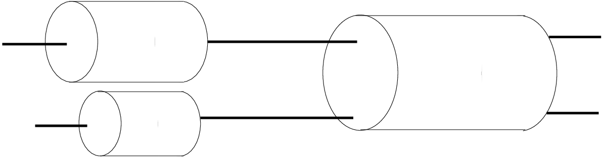
Consider for example the tree network represented on the left of Figure 1, with two traffic routes, each passing through a dedicated link, followed by a common link. If each dedicated link has a capacity , , and the common link has capacity , the flow on each route gets a capacity that lies in the polyhedron :
| (10) | ||||
| (11) |
Another example of interest is the linear network represented on the right of Figure 1 with routes sharing two links. While the first route passes through both links, routes and only use one of the links (one each). This gives the following capacity constraints:
| (12) | ||||
| (13) |
In general, like for the specific foregoing examples, the capacity constraints determine the space over which a network controller can choose a desired allocation function. It has been argued by (Kelly, Maulloo and Tan, 1998) that a good approximation of current congestion control algorithms such as TCP (the Internet’s predominant protocol for controlling congestion) can be obtained by using the weighted proportional fair allocation, which solves an optimization problem for each vector of instantaneous numbers of flows. Specifically, the weighted proportional fair allocation for state vector maximizes
where the weights are class-dependent control parameters.
Remark 4.1.
By definition of this optimization program, if is the standard (unweighed) proportional fair allocation with , then the allocation corresponds to the weighted proportional fair allocation with weights .
This framework has been generalized to so-called weighted -fair allocations, which provide flexibility to model different levels of fairness in the network. Another important alternative is the balanced fair allocation (Bonald et al., 2006), which allows a closed form expression for the stationary distribution of the numbers of flows in progress. In addition, the balanced fair allocation gives a good approximation of the proportional fair allocation while being easily evaluated, which is attractive for performance evaluation.

Remind that all -fair bandwidth sharing are stable for (in the sense that the process is positive recurrent) (Bonald and Massoulié, 2001; de Veciana, Konstantopoulos and Lee, 2001) if
We now refine the concept of stability by saying that the network is stable if classes undergoing a surge eventually drain while the other classes stay stochastically stable. More formally, we say that
Definition 4.1.
The network is robust stable if:
Define further the robust stability region as the set of parameters such that the network is robust stable, i.e.:
| (14) |
In the sequel, we first show that for work-conserving allocations, the robust stability set coincides with the usual stability set (except possibly on a negligible set of parameters).
On the other hand, the situation is much more complex for non-work-conserving allocations where even with appropriate weighted allocations, surges might not be asymptotically transparent to the other classes while classes undergoing surges might get asymptotically strictly more bandwidth than in the case of the allocation giving full priority to stable classes. We give an example of this phenomenon later on.
For monotonic networks, we however prove that the robust stability coincide with the set of parameters under which a “priority allocation” is stable.
4.2 Existence of the fluid limit
Lemma 4.1.
If , then the processes are positive recurrent for any , and Theorem 3.1 applies.
Proof. Asymptotically, when the allocation allocated to classes coincides with the allocation which is stable under the usual conditions of traffic.
4.3 Work-conserving allocations
Consider a work conserving allocation such that
Every work-conserving allocation has the same stability region, namely
If the (usual) stability condition is satisfied, then the priority mechanism considered is asymptotically equivalent to giving full priority to class-. In other words, the fluid limit obtained for class- is in that case the same as the fluid limit of an allocation that gives a full priority to class-, which we prove in the following Proposition.
Proposition 4.1.
For a work conserving network, (except possibly on the frontier of the stability sets) and:
Proof. Assume in which case the network is stable. Fix . Using the conservation of the rates at equilibrium for the process ( which boils down in the Markovian context to saying that at equilibrium the drift of should be ), we can write that:
We now calculate for :
Hence, the capacity seen asymptotically by class- is (), which concludes the proof.
Example: one link with the DPS allocation
The simplest instance of a network consists of one link shared by several competing classes of traffic. If the initial policy is supposed to be the classical processor sharing policy: then the prioritized version of the model becomes the so-called discriminatory processor sharing (DPS):
Consider a single link of capacity shared by three classes. The bandwidth is allocated according to DPS with weight for class , . Proposition 4.1 says that is a straight line with slope . This behavior is illustrated in Figure 2, for which . The slope calculated using the proposition is thus , which is verified in the figure.


In Figure 2, we plot the empirical mean of class- at a macroscopic scale, (i.e. ) for a temporal window of .
4.4 Monotone allocations
Define the allocation giving full priority to class to , given by
Denote the stability region of the network with allocation .
Proposition 4.2.
Consider a monotonic allocation (i.e. such that is decreasing in , ).
If where is defined by (9), then the network is robust stable and surging classes do not influence asymptotically stable classes. Conversely if , the network is not robust stable.
Moreover if the network with allocation is stable i.e.:
Proof. Using stochastic comparisons (see (Borst, Jonckheere and Leskelä, 2008) for more details on stochastic comparisons of multidimensional birth-and-death processes with monotonic allocations), we obtain that
which implies that This in turn implies that
This implies that will reach 0 in finite time.
The reverse statement follows along the same lines.
Example: a tree network
Let us consider the tree network shown in Figure 1 with and . We shall assume the following bandwidth allocation: Define . For and ,
| (15) |
and .
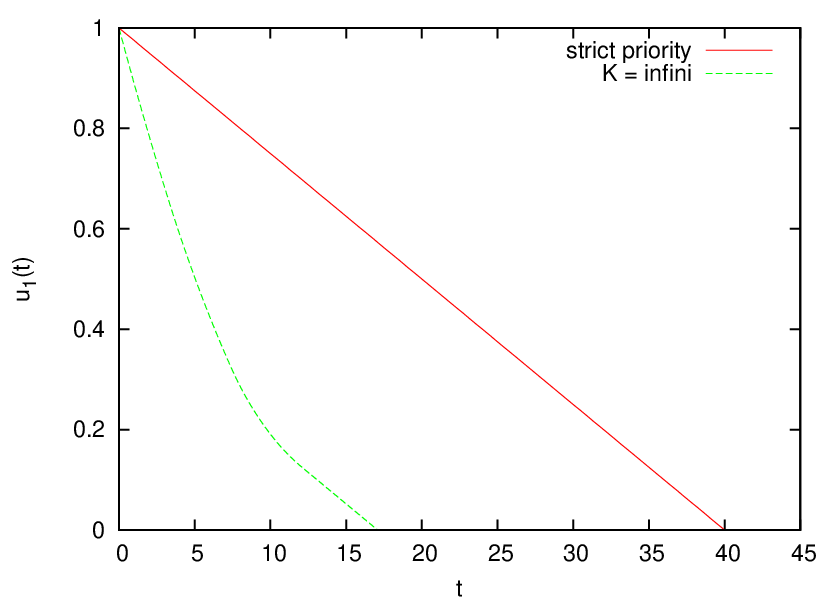
For this network, the allocation becomes a strict priority allocation for class- when , in which case class- gets capacity if there are no class- flows, and otherwise. Thus, for a fixed value of , class- is stable if . The stability regions for and are shown in Figure 3.

The dynamics of for two different values of – one in each region – is plotted in Figure 4, for which .


For class , when the priority allocation is stable the dynamics of the average number of customers converges to the one of the priority allocation, that is , as is illustrated in Figure 4.
In Figure 5, we show how class- is actually favored by asymptotically using the bandwidth of class-, compared to the case where class- is given a strict priority.
4.5 Non-monotone networks
For non-monotonic networks, some unusual behaviors can be observed; for instance the usual fluid limit may exhibit the following behavior: one class of traffic can reach at the fluid scale and stay at 0 for a finite time before increasing again. We here show on an example how the priority scaling avoids this kind of behavior.
Here, we consider a linear network with two links and three classes of flows as shown in Figure 1.
Let be the capacity allocated to a flow of class-. The capacity allocated to class-, , is then . The bandwidth is allocated according to the weighted proportional fair allocation, that is, is the solution of the following maximization problem:
where is the weight of class .
Consider the following network parameters with arrival rates and service rates:
that is, the three classes are unstable at the beginning. The trajectories of the number of flows as a function of the scaled time for is shown in Figure 6.


Concerning the usual fluid limit, we observe that Class becomes stable around the time unit mark. It then becomes unstable around the time unit mark, and becomes stable again around the time unit mark. This behavior can be explained as follows.
In the first part of the trajectory, class gets sufficient capacity to drain out while the number of class flows grows. In the second part, since Link is not a bottleneck for Class flows and Class gets smaller, Class gets a larger share on Link . Meanwhile, the arrival and service rates of Class and Class being the same, the imbalance in the rate allocation means that Class is now unstable and its number of flows starts to grow until it reaches the same number as that of Class flows at which time they both share the link capacity equally. Since the network is stable, all the three classes drain out eventually.
Due to the priority mechanism employed to penalize unstable classes, such a phenomenon does not happen in the case of the priority scaling as illustrated in the right-hand Figure.
5 Integration of streaming and elastic traffic
Consider now a system where two intrinsically different types of traffic – “streaming” and “elastic” traffic – coexist and share a given link. Such models have been considered by (Nunez-Queija, van den Berg and Mandjes, 1999; Delcoigne, Proutière and Régnié, 2004; Bonald and Proutière, 2004). It is natural to equip streaming traffic with a fixed required rate, say, per flow. Giving priority to streaming traffic (class 2) the allocation of service may be chosen as:
where the parameter quantifies the level of priority. The allocated capacity cannot exceed the total capacity. If the latter is normalized to 1, the state space must be restricted to states such that
Then, if the number of current streaming flows is such that arriving streaming flows must be blocked from the network.
In this example, if accepted in the network, the capacity allocation of class- flows is independently of the number of flows of class-, for all values of , whereas the capacity allocation of class- flows depends on the number of class- flows such that . However, class- flows are admitted only if there is sufficient capacity, that is, if .
Denote
the state space of class- conditioned on . Define . The process is birth-death process with birth rate and death rate , and whose stationary distribution is given by
For the priority allocation, class- is stable if and only if . Thus, if , then the limit point of is , and if , then the limit point is positive.
Performing the scaling previously defined, remark that the state space depends for a fixed macroscopic state on both and . We can apply Theorem 3.1 with being defined by:
where . In the case that is very small (), we might consider as a reasonable approximation a Poisson distribution for class-, whatever the state of class-. In that case, takes a slightly simpler form. After simple calculations:
This allows a recursive evaluation for integer-valued . Using simple calculus, for :
We can also evaluate in terms of special functions:
where is the incomplete function.
In Figure 7, we plot the for , , and .

5.1 Quality-of-Service guarantee
The Quality-of-Service for streaming flows is mainly characterized by the probability that an incoming flow does not find sufficient capacity in the network for the flow to be accepted. In networks in which streaming and elastic traffic do not interact, this probability can be computed using an Erlang Fixed-Point approximation (Kelly, 1986). However, in the context of the present example, the interaction of these two types of traffic makes it more difficult to apply these fixed-point approximations, mainly due to the fact that the state space of the elastic flows is unbounded. However, in the limiting regime under consideration, we can come up with a rule-of-thumb that can be used to guarantee a blocking probability smaller than a desired value.
First, we consider a single link whose capacity is shared by the two types of flows. Let denote the desired maximal blocking probability of class- flows. We shall set the priority level of class- (by varying ) such that the probability of blocking of class- is always less than .
For , an arrival of class- is blocked if and only if , which is equivalent to . The term is the number of circuits of size available when the total capacity is . Thus,
is the maximum number of simultaneous flows of class- in the system, and an arrival of class- is blocked if and only if the number of flows of class- is .
Let denote the blocking probability when the number of circuits is the network is . From the Erlang-B formula,
The inverse function gives the minimum number of circuits required to ensure a blocking probability smaller than . In order to guarantee a maximal blocking of the number of circuits, has to be larger than at all instant of time, which leads us to the following necessary and sufficient condition for guaranteeing the Quality-of-Service of class- flows:
We can ensure the above inequality by scaling the process by a factor . This, in turn, can be achieved by scaling the priority level (or, equivalently, ) by this very same factor. This additional scaling results in a larger share of the bandwidth for class- flows in case . Conversly, if , the priority level of class- flows is appropriately decreased so that the blocking probability constraint of class- flows is not violated.
Using the monotonicity of in its first variable, we get that if , then converges monotonically to its limit point. Hence,
Remark 5.1.
The blocking probability for a given value of is in fact a conditional blocking probability in the sense that it is the fraction of calls dropped when the class- flows take away a capacity of . The unconditional blocking probability of class- flows can be computed by integrating over , which is rather conservative. An alternative scaling could be constructed such that only the unconditional blocking probability satisfies a given constraint.
Remark 5.2.
In a network of links shared by several classes of streaming flows and one class of elastic flow, we could use fixed-point approximations to compute the blocking probability for the different classes of streaming flows as a function of . Assuming that this probability is increasing in , we could then compute the maximum value that can attain without the streaming classes violating their individual blocking probability.
6 Conclusions
We analyzed the flow-level performance of multi-class communication networks when one of the classes undergoes a traffic surge. We showed that, under an appropriate scaling of space and time, the dynamics of the temporarily unstable class can be described by a deterministic differential equation in which the time derivative at a given point depends on the conditional stationary distribution of the other classes calculated at that point. For work-conserving allocations, the differential equation is the same as the one of the network in which other classes have strict priority over the temporarily unstable class, that is, the scaled process evolves linearly and is either absorbed at zero or grows indefinitely depending on whether the network is stable or not.
For non-work conserving allocations, the trajectory is much more complex to describe as it depends on the mean residual bandwidth left over by the other classes which in turn depends on the current state of the first class. The limit point of the fluid trajectory can hence be non-zero and finite. We characterized the robust stability region of monotone allocations. We illustrated this behavior through several examples of network topologies and bandwidth allocations that are commonly used to model communication networks.
The time-space-transitions scaling that we considered raises several open questions which would give a better understanding of the network dynamics. In particular, finding necessary and sufficient conditions for the limit point of non work-conserving allocations to be zero would constitute a very interesting result. Also, error bounds estimates would be necessary to obtain a reliable performance evaluation tool.
Acknowledgment
We would like to thank A. Ferragut and F. Paganini for fruitful discussions on the example 4.5.
References
- Billingsley (1999) [author] Billingsley, PatrickP. (1999). Convergence of Probability Measures (second edition). Wiley Series in Probability and Statistics. Wiley-Interscience.
- Bonald and Massoulié (2001) Bonald, T. and Massoulié, L. (2001). Impact of fairness on Internet performance. In SIGMETRICS’01.
- Bonald and Proutière (2003) [author] Bonald, T.T. and Proutière, A.A. (2003). Insensitive Bandwidth Sharing in Data Networks. Queueing Syst. Theory Appl. 44 69–100.
- Bonald and Proutière (2004) Bonald, T. and Proutière, A. (2004). On performance bounds for the integration of elastic and adaptive streaming flows. In SIGMETRICS 235-245.
- Bonald et al. (2006) [author] Bonald, T.T., Massoulié, L.L., Proutière, A.A. and Virtamo, J.J. (2006). A queueing analysis of max-min fairness, proportional fairness and balanced fairness. Queueing Syst. Theory Appl. 53 65–84.
- Borst, Jonckheere and Leskelä (2008) [author] Borst, S. C.S. C., Jonckheere, M.M. and Leskelä, L.L. (2008). Stability of parallel queueing systems with coupled service rates. Discrete Event Dyn. Syst. 18 447–472.
- C. Kipnis (1991) [author] C. Kipnis, C. LandimC. L. (1991). Scaling limits of interacting particle systems. Springer.
- Dai (1995) [author] Dai, J. G.J. G. (1995). On Positive Harris Recurrence of Multiclass Queueing Networks: A Unified Approach Via Fluid Limit Models. Annals of Applied Probability 5 49–77.
- Darling and Norris (2008) [author] Darling, R. W. R.R. W. R. and Norris, J. R.J. R. (2008). Differential equation approximations for Markov chains. Probability Surveys 5 37.
- de Veciana, Konstantopoulos and Lee (2001) [author] de Veciana, GustavoG., Konstantopoulos, TakisT. and Lee, Tae-JinT.-J. (2001). Stability and performance analysis of networks supporting elastic services. IEEE/ACM Trans. Netw. 9 2–14. http://dx.doi.org/10.1109/90.909020
- Delcoigne, Proutière and Régnié (2004) [author] Delcoigne, F.F., Proutière, A.A. and Régnié, G.G. (2004). Modeling integration of streaming and data traffic. Perform. Eval. 55 185–209.
- Deshpande et al. (2007) [author] Deshpande, M.M., Amit, A.A., Chang, M.M., Venkatasubramanian, N.N. and Mehrotra, S.S. (2007). Flashback: A Peer-to-Peer Web Server for Flash Crowds. International Conference on Distributed Computing Systems 15.
- Ethier and Kurtz (1986) [author] Ethier, Stewart N.S. N. and Kurtz, Thomas G.T. G. (1986). Markov Processes: Characterization and convergence. Wiley.
- Feuillet (2010) [author] Feuillet, MathieuM. (2010). On the stability of linear networks and upstream trees without congestion control mechanisms. submitted.
- Gromoll and Williams (2009) [author] Gromoll, H. C.H. C. and Williams, R. J.R. J. (2009). Fluid limits for networks with bandwidth sharing and general document size distributions. Annals of Applied Probability 19 243.
- Hartman (1960) [author] Hartman, PhilipP. (1960). A lemma in the theory of structural stability of differential equations. Proc. A.M.S. 11(4) 610–620.
- Jonckheere, Nunez-Queija and Prabhu (2010) Jonckheere, M., Nunez-Queija, R. and Prabhu, B. (2010). Performance Analysis of Traffic Surges in Multi-class Communication Networks. In ITC 22.
- Kandula et al. (2005) Kandula, S., Katabi, D., Jacob, M. and Berger, A. . W. (2005). Botz-4-Sale: Surviving Organized DDoS Attacks That Mimic Flash Crowds. In 2nd Symposium on Networked Systems Design and Implementation (NSDI).
- Kelly (1979) [author] Kelly, F.F. (1979). Reversibility and Stochastic Networks. Wiley.
- Kelly (1986) [author] Kelly, F.F. (1986). Blocking probabilities in large circuit-switched networks. Adv. Appl. Probab. 18 473–505.
- Kelly, Maulloo and Tan (1998) [author] Kelly, F. P.F. P., Maulloo, A. K.A. K. and Tan, D. K. H.D. K. H. (1998). Rate Control for Communication Networks: Shadow Prices, Proportional Fairness and Stability. The Journal of the Operational Research Society 49 237–252.
- Kurtz (1992) Kurtz, T. G. (1992). Averaging for martingale problems and stochastic approximation. In Applied Stochastic Analysis, US-French Workshop. Lecture notes in Control and Information sciences 177 186–209. Springer Verlag.
- Massoulié and Roberts (2002) [author] Massoulié, L.L. and Roberts, J.J. (2002). Bandwidth sharing: objectives and algorithms. IEEE/ACM Trans. Netw. 10 320–328.
- Meyn (2008) [author] Meyn, S.S. (2008). Control techniques for complex networks. Cambridge University Press.
- Nunez-Queija, van den Berg and Mandjes (1999) Nunez-Queija, R., van den Berg, J. and Mandjes, M. (1999). Performance evaluation of strategies for integration of elastic and stream traffic. In ITC 16 1039-1050.
- Robert (2003) [author] Robert, PhilippeP. (2003). Stochastic Networks and Queues. Stochastic Modelling and Applied Probability Series. Springer-Verlag, New York. xvii+398 pp.
- Rogers and Williams (1987) [author] Rogers, L. C. G.L. C. G. and Williams, D.D. (1987). Diffusions, Markov processes & martingales vol. 2: Itô Calculus. Cambridge University Press.
- Segel and Slemrod (1989) [author] Segel, Lee AL. A. and Slemrod, M.M. (1989). The Quasi-Steady-State Assumption: A Case Study in Perturbation. SIAM Review 31 446–477.
- Stavrou, Rubenstein and Sahu (2004) [author] Stavrou, A.A., Rubenstein, D.D. and Sahu, S.S. (2004). A lightweight, robust P2P system to handle flash crowds. Selected Areas in Communications, IEEE Journal on 22 6–17.