Real Space Green’s Function Approach to RIXS
Abstract
We present an ab initio theory of core- and valence resonant inelastic x-ray scattering (RIXS) based on a real-space multiple scattering Green’s function formalism and a quasi-boson model Hamiltonian. Simplifying assumptions are made which lead to an approximation of the RIXS spectrum in terms of a convolution of an effective x-ray absorption signal with the x-ray emission signal. Additional many body corrections are incorporated in terms of an effective energy dependent spectral function. Example calculations of RIXS are found to give qualitative agreement with experimental data. Our approach also yields simulations of lifetime-broadening suppressed XAS, as observed in high energy resolution fluorescence detection experiment (HERFD). Finally possible improvements to our approach are briefly discussed.
Keywords:
RIXS,XAS,XESpacs
78.70.Dm,78.70.En,78.70.CkI Introduction
Resonant inelastic x-ray scattering (RIXS) is a powerful tool for probing occupied and unoccupied densities of states at high resolution. Moreover, the RIXS signal contains valuable information about the many-body excitations of a system, e.g., those beyond the primary quasi-particle excitation.[1, 2, 3, 4] However, because the RIXS signal is described by the Kramers-Heisenberg equation rather than Fermi’s golden rule and is sensitive to many-body excitations, theoretical calculations of RIXS are more difficult than those of related core-level spectroscopies such as x-ray absorption (XAS), x-ray emission (XES), and electron energy loss (EELS). Even so, models of the RIXS spectrum based on single particle band structure arguments can be quite useful for systems with weak electron correlations, i.e., -electron systems.[5, 6, 7, 8, 9, 10, 11, 12] In order to account for particle-hole interactions, methods based on the Bethe-Salpeter equation have been employed.[13] In addition, there have been works modeling -electron systems within the single particle picture.[14, 15, 16] Also, for systems with strong electron correlations, the Anderson impurity model and atomic multiplet theories have been used to explain RIXS spectra of localized and -state systems.[17] For more detailed reviews see e.g., Ref. 2, 3, 4.
In this paper we introduce a theoretical treatment of RIXS based on an approximation to the Kramers-Heisenberg equation which uses a real space multiple-scattering Green’s function (RSGF) formalism to describe the single particle spectrum and a quasi-boson model Hamiltonian to account for multi-electron (e.g. shake-up and shake-off) excitations.[18, 19] Although extensions are possible, our approach is currently limited to systems with weak correlations. Our derivation is similar in some respects to that of Ref. 12, which also uses a multiple-scattering formalism and a related treatment of inelastic losses. The main differences are: i) our expression does not rely on a single site approximation for the single particle Green’s function; ii) we include quasi-particle self-energy corrections based on a many-pole model of the dielectric function; and iii) we approximate the many-body losses via a convolution with an effective spectral function that includes intrinsic and extrinsic losses and interference effects.[19] In addition, with several simplifying assumptions, we demonstrate that the RIXS cross section can be approximated as a convolution of XAS and XES signals. This simplified formula is analogous to an expression in terms of appropriate joint densities of states. [14, 15] However, our result also explicitly includes the energy dependence of the dipole matrix elements. In order to calculate our approximation to the RIXS spectrum efficiently, we have implemented the theory in an extension of the real space multiple-scattering Green’s function code FEFF9.[20, 21] This RSGF technique has already been used to calculate several other core-level spectroscopies, including XAS, XES and EELS, as well as VIS-UV spectra.[21, 22, 23, 24] The RSGF method has been particularly beneficial for the core-level spectroscopies of complex systems, since it does not rely on periodic symmetry, which is generally broken by the presence of the core hole. Moreover, the approach is applicable over a broad range of energies. Illustrative examples are presented which yield reasonable agreement with available experimental RIXS. Our theory also yields simulations for related spectra, e.g., lifetime broadening suppressed x-ray absorption spectra, as observed in high energy resolution fluorescence detection (HERFD) experiments.
The remainder of this article is ordered as follows. We begin by introducing the theory of RIXS based on the Kramers-Heisenberg equation and then summarize our key results. In particular we derive an approximate formula for the RIXS cross section in terms of a convolution of XES and effective XAS signals. We then present a more detailed derivation of RIXS in terms of quasi-particle Green’s functions within the RSGF formalism. Subsequently, we present several illustrative calculations and compare with experimental data in a number of weakly correlated systems. Although our treatment is in principle more general, we restrict our attention in this work to systems for which the quasi-particle approximation is reasonable. Finally, we make a number of concluding remarks. Technical details are relegated to the Appendices.
II Theory
II.1 RIXS in terms of XAS and XES
Below we briefly outline the basic theory of RIXS and describe the key expressions used in our calculations. All quantities are expressed in Hartree atomic units () unless otherwise noted. Formally the resonant inelastic x-ray scattering double differential cross section is given by the Kramers-Heisenberg formula[25]
| (1) |
Here and are the energies of the incoming and outgoing photons; and are the many-body transition operators; and , and are many-body electronic ground, intermediate, and final states with corresponding energies , , and . This formula for the cross section can be expressed in terms of effective one particle Green’s functions [cf. Ref. 12 and our derivation in Sec. (II.3)] corresponding to the intermediate and final many-body states
| (2) |
Here the one-particle Green’s functions and are given by
| (3) |
where and denote deep and shallow core holes, is the ground state of the valence electrons in the presence of core hole , the projection operators and project onto unoccupied or occupied states of the single particle ground state Hamiltonian, and , are the core level energies. As shown in Appendix A, we can rewrite this expression in terms of a non-local transition operator
| (4) |
where We now relate this result to the x-ray emission and an x-ray absorption like signal .
| (5) |
where the effective absorption coefficient is
| (6) |
The quantity differs from normal x-ray absorption coefficient since the dipole transition operator in XAS is replaced by . If the matrix elements of are much smaller than unity, which is the case for all but localized excitations, we may take the leading order approximation, and thus relate the RIXS to the usual x-ray absorption coefficient , i.e.,
| (7) |
Thus we obtain a relatively simple expression for the RIXS cross section in terms of the x-ray absorption, x-ray emission, and a resonant denominator. Moreover, the terms in either expression [Eq. (5) or (7)] can be calculated within the RSGF framework, as in the FEFF codes.[20, 26, 23, 27, 21] It should be noted that the above expressions (Eq. 5 and 7) are similar to those given in the pioneering work of Tulkki and Åberg,[28, 29, 30] in which a derivation of electronic resonant Raman spectra is given in terms of multichannel scattering states, and applied to the K-alpha RIXS of KMnO4.
II.2 Multiple Scattering Theory
We now turn our attention to the application of the multiple-scattering RSGF formalism to Eq. (5). Within this formalism the single particle Green’s function can be expanded about the absorbing atom (see Ref. 20)
| (8) |
Calculations of the RIXS cross section require both the single particle XES signal, which is relatively simple to calculate with FEFF9, and the effective absorption cross-section . In order to calculate the latter we begin by rewriting Eq. (6) in terms of the one-electron density matrix ,
| (9) |
Note again that and signify states calculated in the presence of the deep or shallow core hole respectively. Using the fact that and inserting our expression for the Green’s function, we obtain
| (10) |
where we have assumed that the argument is real, and used the result for energies on the real axis. Note that the energy arguments of the bras and kets have been omited above for the sake of brevity. We now turn to the matrix elements of the transition operator
| (11) |
where for simplicity, we have neglected the projection operator , i.e. approximated =1. Then rewriting the Green’s function in spectral representation, and again inserting the MS expression for the Green’s function in Eq. (8) gives
| (12) |
Thus in addition to the usual dipole matrix elements, we have a second term which depends on both energies in the problem, the incoming photon frequency and the energy loss .
II.3 Many-Body Effects and the Quasi-Boson Model
In this subsection we discuss the application of the quasi-boson model[31] to calculations of inelastic loss effects in RIXS. Assuming that the absorption occurs from a deep core level and employing the dipole approximation for the transition operators in Eq. (1) gives
| (13) |
If we neglect exchange terms between the particle and hole, or at least assume that they are dealt with via an effective single particle potential, we can write the many-body ground state as
| (14) |
where is associated with a specific term in the sum over states in , is the deep core state excited by the absorption event, and is an electron wave-function. Note that this approximation is only justified if denotes a core electron or a high energy photo-electron, although we will use the approximation for valence electrons as well. This gives
| (15) |
where and
| (16) |
Note that is now the Fermi energy. Then the RIXS cross section becomes
| (17) |
where , , and is given by
| (18) |
and is the many-body Green’s function. We now introduce a quasi-boson approximation to the Hamiltonian following the treatment of Ref. 18. In this approach the excitations of the many-body valence electronic state are represented as bosons while the photo-electron and hole are treated via an effective single-particle theory
| (19) |
where and are the one-particle Hamiltonians for the hole and particle respectively, describes the interaction of the hole/particle with the valence electrons,
| (20) | ||||
| (21) | ||||
| (22) |
and describes the interaction between the photo-electron and hole. This last interaction term should in principle be treated via the Bethe-Salpeter equation; however, here we will approximate it using either a self-consistent final state rule approximation for deep core holes (i.e., with the screened core-hole potential of the deep core-hole), or by neglecting it altogether, as in the initial state rule (independent particle approximation) for valence holes. Experience with such models in the FEFF code shows that these approximations are reasonable.
We now define as the ground state of the electron system in the presence of the deep core hole , and as the ground state of the electron system in the presence of the second core hole so that
| (23) |
with core level energies
| (24) |
The transition matrix elements corresponding to emission () may be pulled outside the imaginary part, and serve as an amplitude factor, i.e.,
| (25) |
Here , , is a projector onto unoccupied states of the ground state Hamiltonian, is a projector onto occupied states of the intermediate state Hamiltonian,
| (26) |
and finally, the Green’s functions are calculated in the presence of the deep () or shallow () core hole, i.e.,
| (27) |
Next we derive an expression for the effects of multi-electron excitations in terms of an effective spectral function. Within the quasi-boson approximation, the following relationships between the eigenstates of , , and hold[19, 18]
| (28) |
Here is the difference between the intermediate and final state core hole potentials. If we assume only single boson excitations, we can also write
| (29) |
which will give us the correct expression to second order in the couplings when used in our formula for the RIXS signal. Ignoring the off-diagonal terms in we obtain
| (30) |
Note that in the case of valence emission (valence hole), we are assuming that the core hole potential is negligible, hence , and . Expanding to second order in the amplitudes to create and annihilate bosons, and neglecting off resonant terms, gives the total cross section in terms of a convolution with an effective spectral function .
| (31) |
where is the single particle cross section as given in Eq. (5), and the spectral function is given by
| (32) |
Here , are the amplitudes to create or annihilate a bosonic excitation, respectively, and include extrinsic as well as intrinsic amplitudes (see Appendix B). It should be noted that our current formalism for the spectral function is not suited for highly correlated materials, although an extension of the quasi-boson model Hamiltonian is possible, as suggested in Ref. 31 and 32.
The application of the spectral function to RIXS is similar to that of Ref. 18 and 19, where a convolution was applied to XAS. In this paper, however, we will restrict our calculations to the quasiparticle approximation, i.e., with the spectral function replaced by a -function,
| (33) |
The use of this approximation is expected to cause the calculated spectral line-shapes to be more symmetric than experimental results, since the main quasiparticle peak is modeled in the above as a Lorentzian, while in general multi-electron excitations lead to asymmetric peaks so that Eq. (32) has a Fano type main lineshape. Thus satellite peaks due to multi-electron excitations are also neglected.
III Experiment
The experiments described here were performed at beamline ID26 of the European Synchrotron Radiation Facility (ESRF). The incident energy was selected by means of a pair of cryogenically cooled Si crystals in () reflection with an energy bandwidth of eV ( eV) at keV ( keV). The incident flux on the sample was photons/second using the fundamental peak of the undulator radiation. The beam size on the sample was mm vertical by mm horizontal. Higher harmonics were suppressed by three Si mirrors operating in total reflection. The resonantly scattered x-rays were analyzed using the () and () reflection of spherically bent Ge single crystal wafers for the Ti and emission, respectively. The Ge () reflection was used for Mn . Sample, analyzer crystals and an avalanche photo diode were arranged in a vertical Rowland geometry ( m) at deg scattering angle. The combined instrumental energy bandwidth was eV. All samples were purchased from Aldrich and used as is. Self-absorption effects distort the spectral shape and let the K absorption pre-edge region appear stronger relative to the edge jump. These effects are negligible in the K absorption pre-edge region and the samples were not diluted for the measurements.

IV Results and Discussion
IV.1 RIXS
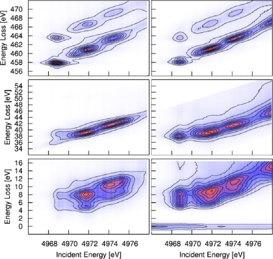
Calculations of RIXS were carried out for several materials based on the present theoretical approach using an extension of the RSGF FEFF9 code applied to Eq. (31). All results were calculated using self-consistent potentials and a full multiple scattering (FMS) treatment of the Green’s functions for suitably large clusters centered at the core absorption site. The core-hole screening was calculated using the random phase approximation (RPA),[34] and non-spherical parts of the core-hole potential were neglected. In order to simplify the calculations the Green’s functions are restricted to include only the site and angular momentum diagonal elements. We find that for the cases presented here, the angular momentum diagonal approximation is reasonable for all but the lowest energy peaks since the overlap with is then small, and our approximation then becomes equivalent to Eq. (7) in terms of XES and XAS where the angular momentum diagonal elements dominate due to dipole selection rules. To obtain better agreement with the the experimental threshold energy, we allowed a small shift of the calculated Fermi energy, which is typically too high by about 1 eV in the self-consistent FEFF9.0 calculation. In addition, overall energy shifts were added in each axis in order to align the calculation with the energy scale in the experiment. In the case of RIXS, atomic values were used for the splitting between the and emission energies.[35] In addition the amplitudes were taken (from simple counting arguments) to have a ratio , although this ratio is not generally accurate, since the particle-hole interaction mixes the hole states. Fig. 1 presents a comparison of our calculated (right) Mn RIXS of MnO and experimental data (left). The overall agreement is qualitatively satisfactory: all main features of the experiment are reproduced including both the dipole as well as quadrupole pre-edge peaks. The main edge is also at about the correct energy, although the asymmetry caused by multi-electron excitations is absent in our calculation which is restricted to the quasiparticle level where the spectral function is given by Eq. (33). We expect that going beyond this quasi-particle approximation for the spectral function as in Eq. 32 would capture some of the asymmetry since the Lorentzian spectral shape currently used for the quasiparticle peak in these calculations would be replaced by a Fano type lineshape. In addition, new features could arise due to satellite peaks in the spectral function. The main diagonal structure in our calculation appears to be sharper that that of the experiment; this is possibly due to self-absorption effects in the experimental data. Note that the pre-edge peak for this case is basically on the diagonal; i.e., the emission energy is the same for the pre-edge peak as for the main edge.
Core-hole effects are important for a variety of excited state spectoscopies, including EELS and XAS as well as RIXS.[1, 36] RIXS spectra in particular however, can give us insight into these effects since the intermediate and final states have different core-holes.[37] In order to illustrate the effect of different final state core-holes, we calculated the RIXS for Ti , , and RIXS of TiO2 Anatase. In order to obtain reasonable results for the quadrupole peak in the K-edge absorption, we increased the strength of the core-hole potential by using screened core-hole and bare core-hole, and kept the same ratio for all core-hole calculations. Note that our calculation again reproduces all peaks, although the intensity of the calculated quadrupole peaks is weak compared to that observed in the experiment. There is also a noticeable effect on the spectrum due to changes in final state core-hole. For the RIXS, the intermediate () and final () core-holes are both quite localized and the difference is small, thus peaks should occur roughly on the diagonal, as seen by Eq. (12). For the spectrum the final state has a core hole, and the core-hole potential has a vastly different shape than the core-hole potential. This causes to be large, and we expect off diagonal peaks to be present. This is indeed the case, although only the quadrupole peaks are off diagonal. This is due to the fact that the dipole pre-edge peaks are caused by hybridization between the absorbing atom and neighboring Ti atoms, and thus are relatively unaffected by the core-hole potential. The quadrupole peaks, however, are due to a direct transition to the Ti states which are localized around the absorbing atom and are effected by the core-hole potential to a greater extent than the hybridized -states. The effect is also present in the valence spectrum. In addition, the valence spectrum has multiple peaks due to the fact that the emission is from a broad valence band which is split due to solid state effects. The qualitative structure of the valence band is also correct in the calculation, which reproduces the double peak structure with the correct splitting. The intensities are also qualitatively correct with the lower energy-transfer peaks being less intense than the higher energy-transfer peaks. The gap is too small in our calculation, however, this could be accounted for via a GW gap correction. Note that we have not included the elastic scattering contribution in our calculation of the valence RIXS, which could effect the overall asymmetry of the signal. Finally, for all three spectra, the main edge occurs at a larger energy in the calculated results than in the experiment. This could be due to strong correlation effects, which would be expected to shift the Ti -states closer to the -states. Another possible explanation which is important in the case of Ti K pre-edge XAS of Rutile is the failure of the spherical muffin-tin approximation.[36]
IV.2 Lifetime Broadening Suppressed XAS
In addition to the RIXS planes, there are also several methods for obtaining lifetime broadening suppressed (LBS) XAS. In high energy resolution fluorescence detected (HERFD) XAS,[38] an approximate absorption spectrum is found by partial fluorescence yield using a detector with resolution higher than the natural width due to core-hole lifetime effects. This corresponds to viewing the spectra of constant emission energy in the RIXS plane. Another method of obtaining LBS XAS is to set the incident energy at a point well below the edge while scanning the emission energy.[39] Under certain assumptions, the spectrum obtained in this way is approximately proportional to the XAS signal multiplied by a Lorentzian with the width of the intermediate state core-hole. In Fig. 3 we show a comparison of experimental Cr-K edge HERFD XAS of with our calculated results. We find reasonable qualitative agreement, with the exception of the peak just above eV, which is not seen in the calculation. We note however, that the size of this peak is sensitive to distortions. In addition, the amplitude of the main peak after the rising edge is too small. This could be due to the approximate treatment of the core-hole interaction or corrections to the spherical muffin-tin potentials used in FEFF9.


Fig. 4 shows a comparison of bulk metallic Pt L3 edge XANES compared to HERFD XAS and our calculated results. Here we see that all of the features are well reproduced although the broadening is too large at high energies, and the higher energy peaks are also red shifted toward the edge in comparison to the experimental result.
V Conclusions
We have presented a theory of resonant inelastic x-ray scattering (RIXS) which is amenable to practical calculations as an extension of current x-ray-absorption and -emission codes. Starting from the Kramers-Heisenberg equation, we derive an expression for the RIXS cross-section which can be calculated using the real-space Green’s function approach in the FEFF9 code. Inelastic losses and quasi-particle effects are included in terms of an effective spectral-function that is obtained from a quasi-boson model Hamiltonian. These many-body effects are incorporated into a single-particle approximation via a convolution with an effective spectral function. Quasi-particle self-energy effects are included based on a many-pole model of the dielectric function. Approximation of the many-body states as a product of an N-2 electron state with either two core electronic states (i.e. the ground state), or a core and photo-electron state (intermediate and final states) gives the cross section in terms of effective single particle Green’s functions. The further approximation that the intermediate and final photo-electron states are orthogonal with identical energies (valid at high photo-electron energies) gives the signal in terms of a convolution of the XAS and XES spectra. In addition, we have derived a formulation of the core-core RIXS spectrum that, due to the localized nature of , depends primarily on the Green’s functions evaluated close to the absorbing atom. The extent of this localization is yet to be thoroughly investigated, although the degree of agreement between our calculations and experimental data suggests that the on-site approximation is valid for the systems shown here. In addition, the on-site approximation provides good qualitative agreement for the core-valence RIXS, although the approximation is less justifiable. The theory is implemented in an efficient program which is an extension of the FEFF9 real-space multiple-scattering code, which calculates the RIXS spectrum for core-core as well as core-valence RIXS. Several illustrative calculations were presented within the quasi-particle approximation where the spectral function is replaced by a -function, which appears to be a reasonable approximation for these cases. Calculated results for MnO and for Anatase TiO2 based on this quasi-particle approximation are found to agree qualitatively with experimental spectra: the results reproduce both pre-edge and main edge features, the behavior of pre-edge features with varying core-hole interaction strength, and peak structure due to solid state effects in valence RIXS. Further investigations including treatments beyond the quasi-particle approximation of Eq. (33) will be reserved for the future. It should be noted that our current formalism for the spectral function is not suited for highly correlated materials, although an extension of the quasi-boson model Hamiltonian is possible as suggested in Ref. 31 and 32.
Acknowledgements.
We thank T. Ahmed, A. Bansil, R. Markiewicz, E. Shirley, and M. Tromp, for useful discussions. This work was supported by DOE BES Grant DE-FG03-97ER45623 and was facilitated by the DOE Computational Materials and Chemical Sciences Network (JJK and JJR). JAS gratefully acknowledges the financial support from Eemil Aaltonen foundation and Magnus Ehrnrooth foundation. The ESRF is acknowledged for providing beamtime and technical support (PG).References
- [1] P. Glatzel, F. M. F. de Groot, and U. Bergmann, Synchrotron Radiation News 22, 12 (2009a).
- [2] F. de Groot and A. Kotani, Core Level Spectroscopy of Solids (Taylor and Francis CRC press, 2008).
- [3] A. Kotani and S. Shin, Rev. Mod. Phys. 73, 203 (2001).
- [4] W. Schülke, Electron Dynamics by Inelastic X-Ray Scattering (Oxford University Press, 2007).
- [5] Y. Ma, N. Wassdahl, P. Skytt, J. Guo, J. Nordgren, P. D. Johnson, J.-E. Rubensson, T. Boske, W. Eberhardt, and S. D. Kevan, Phys. Rev. Lett. 69, 2598 (1992).
- [6] Y. Ma, Phys. Rev. B 49, 5799 (1994).
- [7] J. A. Carlisle, E. L. Shirley, E. A. Hudson, L. J. Terminello, T. A. Callcott, J. J. Jia, D. L. Ederer, R. C. C. Perera, and F. J. Himpsel, Phys. Rev. Lett. 74, 1234 (1995).
- [8] S. Shin, A. Agui, M. Watanabe, M. Fujisawa, Y. Tezuka, and T. Ishii, Phys. Rev. B 53, 15660 (1996).
- [9] P. D. Johnson and Y. Ma, Phys. Rev. B 49, 5024 (1994).
- [10] K. Kokko, V. Kulmala, J. A. Leiro, and W. Hergert, Phys. Rev. B 68, 052503 (2003).
- [11] J. Luo, G. T. Trammell, and J. P. Hannon, Phys. Rev. Lett. 71, 287 (1993).
- [12] T. Fujikawa, T. Konishi, and T. Fukamachi, J. Electron. Spectrosc. Relat. Phenom. 134, 195 (2004).
- [13] E. L. Shirley, J. A. Soininen, G. P. Zhang, J. A. Carlisle, T. A. Callcott, D. L. Ederer, L. J. Terminello, and R. C. C. Perera, J. Electron. Spectrosc. Relat. Phenom. 114-116, 939 (2001).
- [14] J. Jiménez-Mier, J. van Ek, D. L. Ederer, T. A. Callcott, J. J. Jia, J. Carlisle, L. Terminello, A. Asfaw, and R. C. Perera, Phys. Rev. B 59, 2649 (1999).
- [15] P. Glatzel, J. Singh, K. O. Kvashnina, and J. A. van Bokhoven, J. Am. Chem. Soc. 132, 2555 (2010).
- [16] M. van Veenendaal, Phys. Rev. Lett. 96, 117404 (2006).
- [17] A. Kotani, Eur. Phys. J. B 47, 3 (2005).
- [18] L. Campbell, L. Hedin, J. J. Rehr, and W. Bardyszewski, Phys. Rev. B 65, 064107 (2002).
- [19] J. J. Kas, A. P. Sorini, M. P. Prange, L. W. Cambell, J. A. Soininen, and J. J. Rehr, Phys. Rev. B 76, 195116 (2007).
- [20] J. J. Rehr and R. C. Albers, Rev. Mod. Phys. 72, 621 (2000).
- [21] J. J. Rehr, J. J. Kas, F. D. Vila, M. P. Prange, and K. Jorissen, Phys. Chem. Chem. Phys. 12, 5503 (2010).
- [22] K. Jorissen, J. J. Rehr, and J. Verbeeck, Phys. Rev. B 81, 155108 (2010).
- [23] A. L. Ankudinov and J. J. Rehr, Phys. Rev. B 62, 2437 (2000).
- [24] M. P. Prange, J. J. Rehr, G. Rivas, J. J. Kas, and J. W. Lawson, Phys. Rev. B 80, 155110 (2009).
- [25] H. A. Kramers and W. Heisenberg, Z. Phys. 31, 681 (1925).
- [26] A. L. Ankudinov, B. Ravel, J. J. Rehr, , and S. D. Conradson, Phys. Rev. B 58, 7565 (1998).
- [27] J. J. Rehr, J. J. Kas, M. P. Prange, A. P. Sorini, Y. Takimoto, and F. Vila, C. R. Physique 10, 548 (2009).
- [28] T. Åberg, Phys. Scr. 21, 495 (1980).
- [29] J. Tulkki and T. Åberg, J. Phys. B: At. Mol. Opt. Phys. 13, 3341 (1980).
- [30] J. Tulkki and T. Aberg, J. Phys. B: At. Mol. Opt. Phys. 15, L435 (1982).
- [31] L. Hedin, J. Phys.: Condens. Matter 11, R489 (1999).
- [32] J. D. Lee, O. Gunnarsson, and L. Hedin, Phys. Rev. B 60, 8034 (1999).
- [33] P. Glatzel, U. Bergmann, J. Yano, H. Visser, J. H. Robblee, W. Gu, F. M. F. de Groot, G. Christou, V. L. Pecoraro, S. P. Cramer, et al., J. Am. Chem. Soc. 126, 9946 (2004).
- [34] A. L. Ankudinov, Y. Takimoto, and J. J. Rehr, Phys. Rev. B 71, 165110 (2005).
- [35] J. A. Bearden and A. F. Burr, Rev. Mod. Phys. 39, 125 (1967).
- [36] D. Cabaret, Y. Joly, H. Renevier, and C. R. Natoli, J. Synchrotron Radiat. 6, 258 (1999).
- [37] P. Glatzel, M. Sikora, and M. Fernández-García, The European Physical Journal - Special Topics 169, 207 (2009b).
- [38] K. Hämäläinen, D. P. Siddons, J. B. Hastings, and L. E. Berman, Phys. Rev. Lett. 67, 2850 (1991).
- [39] H. Hayashi, R. Takeda, Y. Udagawa, T. Nakamura, H. Miyagawa, H. Shoji, S. Nanao, and N. Kawamura, Phys. Rev. B 68, 045122 (2003).
- [40] M. Tromp, private communication.
Appendix A Local behavior of RIXS: Derivation of
The RIXS cross section is given in terms of a product of three Green’s functions, i.e., . However, this expression is not very useful, since the spacial arguments of the Green’s function must be integrated over all space to obtain the resonance . In order to see this, imagine that we ignore the core hole potentials in both Green’s functions. In this case, we may write the Green’s functions in spectal representation, and noting that the wave functions are now orthonormal, we may rewrite the above expression as , which is what we expect for energies well above threshold, where the effect of the corehole potential is negligable. While this limit is easy to show analytically, doing so numerically within the real-space MS Greeen’s function formalism proves quite difficult. Below, we derive an alternative expression for the RIXS cross section which takes advantage of the localization of core-hole potential. Let us first define the Hamiltonian operators corresponding to the deep (b) and shallow (c) core holes.
| (34) | ||||
| (35) | ||||
| (36) |
We can use these definitions to rewrite the Green’s funtions as follows
| (37) | ||||
| (38) |
where we have left the energy arguments off of the Green’s functions for the sake of brevity. Using these relations gives
| (39) | ||||
| (40) |
where Applying the above relations to gives
| (41) |
Noting that the second term above is real, we have
| (42) |
Finally, we see that the transition matrix element defined in Section (II) can be related to , i.e.,
| (43) |
Appendix B Effective Spectral function
As shown in Sec. (II), the RIXS cross section is given in terms of the ground state expectation value of a product of three many-body Green’s functions. Here we will derive an expression based on quasi-particle Green’s functions and a many-body spectral function.
| (44) |
Note that if we are expanding to second order in the boson couplings, only containing single boson excitations, contribute. Now,
| (45) |
where and . Thus Eq. (44) becomes
| (46) |
We now define the amplitudes to create a single boson as
| (47) |
and the amplitudes to annihilate a boson as
| (48) |
Then combining Eq. (B3)-(B5) gives six terms quadratic in these amplitudes plus the zeroth order term. If we neglect the off-resonant terms, i.e. those terms which contain a , with different energy arguments, this leaves only two terms plus the zeroth order term,
| (49) |
where , and . This result can now be written in terms of a double convolution with a spectral function, i.e.,
| (50) |
where the effective spectral function is given by
| (51) |