Performance Bounds for Sparse Parametric Covariance Estimation
in Gaussian Models

We consider a Gaussian signal vector $\mathbf{s}\hskip-0.56905pt\in\hskip-0.56905pt\mathbb{R}^{M}\!$, $\mathbf{s}\hskip-0.56905pt\sim\hskip-0.56905pt\mathcal{N}(\bm{\mu},\mathbf{C})$ embedded in white Gaussian noise $\mathbf{n}\hskip-0.56905pt\sim\hskip-0.56905pt\mathcal{N}(\mathbf{0},\sigma^{2}\mathbf{I})$. The observed vector

is

$$\mathbf{y}\hskip 0.56905pt=\hskip 0.56905pt\mathbf{s}+\mathbf{n}\,,\vskip-1.42262pt$$

(1)

where $\mathbf{s}$ and $\mathbf{n}$ are independent and the signal mean $\bm{\mu}$ and noise variance $\sigma^{2}$ are known. In what follows, we assume $\bm{\mu}\!=\!\mathbf{0}$ since a nonzero $\bm{\mu}$ can always be subtracted from $\mathbf{s}$. The signal covariance matrix $\mathbf{C}$ is unknown; we will parameterize it according

to

$$\mathbf{C}\hskip 0.56905pt=\hskip 0.56905pt\mathbf{C}(\mathbf{x})\hskip 0.56905pt\triangleq\hskip 0.56905pt\sum_{k=1}^{N}x_{k}\mathbf{C}_{k}\,,\vskip-1.42262pt$$

(2)

with unknown nonrandom coefficients $x_{k}\!\geq\!0$ and known positive semidefinite “basis matrices” $\mathbf{C}_{k}$. Thus, estimation of the signal covariance matrix $\mathbf{C}$ reduces to estimation of the coefficient vector $\mathbf{x}\triangleq(x_{1},\ldots,x_{N})^{T}\!\hskip-0.56905pt\in\hskip-0.56905pt\mathbb{R}_{+}^{N}$.

Our central assumption is that $\mathbf{x}$ is $S$-sparse, i.e., at most $S$ coefficients $x_{k}$ are nonzero. We can formulate this as

$$\mathbf{x}\in\mathcal{X}_{S,+}\triangleq\big\{\mathbf{x}^{\prime}\!\hskip-0.56905pt\in\hskip-0.56905pt\mathbb{R}_{+}^{N}\hskip 0.56905pt\big|\hskip 0.56905pt{\|\mathbf{x}^{\prime}\|}_{0}\hskip-0.56905pt\leq\hskip-0.56905ptS\big\}\,.\vskip-1.42262pt$$

(3)

The sparsity degree $S$ is supposed known; however, the set of positions of the nonzero entries of $\mathbf{x}$ (denoted by ${\rm supp}(\mathbf{x})$; note that ${|{\rm supp}(\mathbf{x})|=\|\mathbf{x}\|}_{0}\leq S$) is unknown. Typically, $S\!\ll\!N$. We will refer to (1)–(3) as the sparse covariance model (SCM). The SCM and estimation of $\mathbf{x}$ are relevant, e.g., in time-frequency (TF) analysis [1, 2], where the basis matrices $\mathbf{C}_{k}$ correspond to disjoint TF regions and $x_{k}$ represents the mean signal power in the $k\hskip 0.56905pt$th TF region. An application is cognitive radio scene analysis [3].

The problem we will study is estimation of $\mathbf{z}\triangleq\mathbf{g}(\mathbf{x})\hskip-0.56905pt\in\hskip-0.56905pt\mathbb{R}^{K}\hskip-0.56905pt$ from $\mathbf{y}$, where $\mathbf{g}(\cdot)$ is a known function. This includes estimation of $\mathbf{x}$ and, less trivially, of a linear combination of the $x_{k}$. In the TF application mentioned above, the latter case corresponds to a linear combination of the mean signal powers in the various TF regions.

In this paper, building on [4, 5], we use the theory of reproducing kernel Hilbert spaces (RKHS) to derive lower bounds on the variance of estimators of $\mathbf{z}$. The estimators are required to have a prescribed differentiable mean function; this includes the case of unbiased estimation. They are allowed to exploit the known sparsity of $\mathbf{x}$. The RKHS framework has been previously proposed for a fundamentally different problem of sparsity-exploiting estimation in [6].

Sparsity-exploiting estimation of $\mathbf{C}$ and of $\mathbf{C}^{-1}\hskip-0.56905pt$ was considered recently in [7] and in [8], respectively. In both cases, the sparsity assumption was placed on $\mathbf{C}^{-1}\!$, which corresponds to a sparse graphical model for $\mathbf{s}$. Our SCM approach (2), (3) is clearly different: while the coefficient vector $\mathbf{x}$ is assumed sparse, the matrices $\mathbf{C}$ or $\mathbf{C}^{-1}\hskip-0.56905pt$ need not be sparse.

This paper is organized as follows. In Section 2, we review minimum-variance estimation and the RKHS framework. In Section 3, we use RKHS theory to derive lower variance bounds for the SCM. The special case of unbiased estimation is considered in Section 4. Finally, Section 5 presents a numerical comparison of our bounds with the variance of two established estimation schemes.

According to (13), any lower bound on ${\|\gamma\|}^{2}_{\mathcal{H}(R)}$ entails a lower bound on $L_{\gamma}(\mathbf{x}_{0})$. For mathematical tractability, we hereafter assume that the basis matrices $\mathbf{C}_{k}$ in (2) are projection matrices on orthogonal subspaces of $\mathbb{R}^{M}\hskip-0.56905pt\hskip-0.56905pt$. Thus, they can be written as

$$\mathbf{C}_{k}\hskip-0.56905pt\,=\,\hskip-0.56905pt\sum_{i=1}^{r_{k}}\hskip-0.56905pt\mathbf{u}_{m_{k,i}}\hskip-0.56905pt\mathbf{u}_{m_{k,i}}^{T}\,,\hskip 10.00002ptk=1,\ldots,N\,,\vskip-3.69885pt$$

(14)

where ${\{\mathbf{u}_{m}\}}_{m=1,\ldots,M}$ is an orthonormal basis for $\mathbb{R}^{M}\hskip-0.56905pt$

and the sets $\mathcal{U}_{k}\hskip-0.56905pt\triangleq\hskip-0.56905pt{\{\mathbf{u}_{m_{k,i}}\}}_{i=1,\ldots,r_{k}}\!$ are disjoint, so that they span

orthogonal subspaces of $\mathbb{R}^{M}\hskip-0.56905pt\hskip-0.56905pt$. We note that (2) and (14) correspond to a latent variable model $\mathbf{s}=\sum_{k=1}^{N}\mathbf{s}_{k}$ with $\mathbf{s}_{k}=\sum_{i=1}^{r_{k}}\xi_{m_{k,i}}\hskip 0.56905pt\mathbf{u}_{m_{k,i}}$, where the $\xi_{m_{k,i}}$ are independent zero-mean Gaussian with variance $x_{k}$ for all $i$, i.e., $\xi_{m_{k,i}}\!\hskip-0.56905pt\sim\hskip-0.56905pt\mathcal{N}(0,x_{k})$. This is similar to the latent variable model used in probabilistic principal component analysis [10] except that our “factors” $\mathbf{u}_{m}$ are fixed. With (14), the kernel expression in (12) simplifies

to

$$R(\mathbf{x}_{1},\mathbf{x}_{2})\hskip-0.56905pt\,=\,\hskip-0.56905pt\frac{\prod\limits_{k=1}^{N}(x_{0,k}\hskip-0.56905pt\hskip-0.56905pt+\hskip-0.56905pt\sigma^{2})^{r_{k}}}{\prod\limits_{k=1}^{N}\!\big[(x_{0,k}\hskip-0.56905pt\hskip-0.56905pt+\hskip-0.56905pt\sigma^{2})^{2}-(x_{1,k}\!-\hskip-0.56905pt\hskip-0.56905ptx_{0,k})(x_{2,k}\!-\hskip-0.56905pt\hskip-0.56905ptx_{0,k})\big]^{r_{k}/2}}\hskip 0.56905pt\hskip 0.56905pt,\vskip-1.42262pt$$

where, e.g., $x_{0,k}$ denotes the $k\hskip 0.56905pt$th entry of ${\bf x}_{0}$. We will refer to the SCM with basis matrices $\mathbf{C}_{k}$ of the form (14) as the sparse diagonalizable covariance model (SDCM).¹¹ 1 Indeed, for the SDCM, the covariance matrix $\mathbf{C}(\mathbf{x})$ can be diagonalized by a signal transformation $\mathbf{s}^{\prime}\!=\hskip-0.56905pt\mathbf{U}\mathbf{s}$, with a unitary matrix $\mathbf{U}$ that does not depend on the true parameter vector $\mathbf{x}$. It can be shown that, within the SDCM, a sufficient condition for (9)—and, thus, for the existence of a minimum in (6), (8)—is $x_{k}\hskip-0.56905pt\hskip-0.56905pt<2x_{0,k}\hskip-0.56905pt+\hskip-0.56905pt\sigma^{2}$ for all $k\hskip-0.56905pt\in\hskip-0.56905pt\{1,\ldots,N\}$. Therefore, we choose our domain as

$$\mathcal{D}\,=\,\big\{\mathbf{x}\!\in\!\mathcal{X}_{S,+}\hskip 0.56905pt\big|\hskip 0.56905pt\hskip 0.56905ptx_{k}\!<2x_{0,k}\hskip-0.56905pt+\hskip-0.56905pt\sigma^{2}\;\,\forall\,k\hskip-0.56905pt\in\hskip-0.56905pt\{1,\ldots,N\}\big\}\,.$$

Note that $\mathcal{D}$ depends on $\mathbf{x}_{0}$.

We will now derive a lower bound on ${\|\gamma\|}^{2}_{\mathcal{H}(R)}$ for the SDCM. Let us assume for the moment that $\gamma\!\in\!\mathcal{H}(R)$. Consider $L$ functions $v_{l}({\bf x})$, $l=1,\ldots,L$, with $v_{l}\!:\hskip-0.56905pt\mathcal{D}\!\to\!\mathbb{R}$ and $v_{l}\!\in\!\mathcal{H}(R)$, which are orthogonal, i.e., ${\langle v_{l},v_{l^{\prime}}\rangle}_{\mathcal{H}(R)}\!\hskip-0.56905pt=\!0$ if $l\!\neq\!l^{\prime}\hskip-0.56905pt$. Let $\mathcal{V}$ denote the subspace of $\mathcal{H}(R)$ spanned by the $v_{l}$, and $\mathbf{P}_{\!\mathcal{V}}$ the orthogonal projection operator on $\mathcal{V}$. Clearly, a lower bound on ${\|\gamma\|}^{2}_{\mathcal{H}(R)}$ is given by

$${\|\mathbf{P}_{\!\mathcal{V}}\gamma\|}^{2}_{\mathcal{H}(R)}\hskip 0.56905pt\leq\hskip 0.56905pt{\|\gamma\|}^{2}_{\mathcal{H}(R)}\,.$$

(15)

This lower bound can be expressed as

$${\|\mathbf{P}_{\!\mathcal{V}}\gamma\|}^{2}_{\mathcal{H}(R)}\,=\,\sum_{l=1}^{L}\frac{|{\langle\gamma,v_{l}\rangle}_{\mathcal{H}(R)}|^{2}}{{\|v_{l}\|}^{2}_{\mathcal{H}(R)}}\,.$$

(16)

A convenient construction of functions $v_{l}({\bf x})$ is via partial derivatives of $R(\mathbf{x}_{1},\mathbf{x}_{2})$ with respect to $\mathbf{x}_{2}$ [4]. Consider an index set $\mathcal{K}$ containing exactly $S$ indices from $\{1,\ldots,N\}$, i.e., $\mathcal{K}\hskip-0.56905pt\subseteq\hskip-0.56905pt\{1,\ldots,N\}$ and $|\mathcal{K}|\hskip-0.56905pt=\hskip-0.56905ptS$. Furthermore let $\mathbf{p}_{l}=(p_{l,1},\ldots,p_{l,N})\hskip-0.56905pt\in\hskip-0.56905pt\mathbb{N}_{0}^{N}$ be $L$ different multi-indices satisfying $\supp(\mathbf{p}_{l})\hskip-0.56905pt\subseteq\hskip-0.56905pt\mathcal{K}$. We then define

$$v_{l}(\mathbf{x})\,\triangleq\hskip 0.56905pt\frac{\partial^{\mathbf{p}_{l}}R(\mathbf{x},\mathbf{x}_{2})}{\partial\mathbf{x}_{2}^{\mathbf{p}_{l}}}\bigg|_{\mathbf{x}_{2}=\hskip 0.56905pt\mathbf{x}_{0}^{\mathcal{K}}}\,,\hskip 10.00002pt\;l=1,\ldots,L\,,$$

(17)

where $\frac{\partial^{\mathbf{p}_{l}}f(\mathbf{x})}{\partial\mathbf{x}^{\mathbf{p}_{l}}}\triangleq\Big(\hskip-0.56905pt\prod_{k=1}^{N}\hskip-0.56905pt\frac{\partial^{p_{l,k}}}{\partial x_{k}^{p_{l,k}}}\Big)f(\mathbf{x})$ and $\mathbf{x}_{0}^{\mathcal{K}}$ is obtained from $\mathbf{x}_{0}$ by zeroing all entries except those whose indices are in $\mathcal{K}$. It can be verified that the functions $v_{l}$ are orthogonal, i.e.,

$${\langle v_{l},v_{l^{\prime}}\rangle}_{\mathcal{H}(R)}=\hskip 0.56905ptq_{l}(\mathbf{x}_{0})\hskip 0.56905pt\delta_{l,l^{\prime}}Ê\,,$$

(18)

where $q_{l}(\mathbf{x}_{0})=\frac{\partial^{\mathbf{p}_{l}}\partial^{\mathbf{p}_{l}}R(\mathbf{x}_{1},\mathbf{x}_{2})}{\partial\mathbf{x}_{1}^{\mathbf{p}_{l}}\partial\mathbf{x}_{2}^{\mathbf{p}_{l}}}\Big|_{\mathbf{x}_{1}=\hskip 0.56905pt\mathbf{x}_{2}=\hskip 0.56905pt\mathbf{x}_{0}^{\mathcal{K}}}$. Furthermore [4],

$${\langle f,v_{l}\rangle}_{\mathcal{H}(R)}\hskip-0.56905pt\,=\,\hskip-0.56905pt\frac{\partial^{\mathbf{p}_{l}}f(\mathbf{x})}{\partial\mathbf{x}^{\mathbf{p}_{l}}}\bigg|_{\mathbf{x}\hskip 0.56905pt=\hskip 0.56905pt\mathbf{x}_{0}^{\mathcal{K}}}\hskip 10.00002pt\,\text{for any}\;\,f\!\in\!\mathcal{H}(R)\,.$$

(19)

Using (18) and (19) in (16), we obtain

$${\|\mathbf{P}_{\!\mathcal{V}}\gamma\|}^{2}_{\mathcal{H}(R)}\hskip-0.56905pt\,=\,\hskip-0.56905pt\sum_{l=1}^{L}\frac{1}{q_{l}(\mathbf{x}_{0})}\Bigg|\frac{\partial^{\mathbf{p}_{l}}\gamma(\mathbf{x})}{\partial\mathbf{x}^{\mathbf{p}_{l}}}\bigg|_{\mathbf{x}\hskip 0.56905pt=\hskip 0.56905pt\mathbf{x}_{0}^{\mathcal{K}}}\Bigg|^{2}.$$

(20)

Finally, combining (7), (13), (15), and (20), we arrive at the following bound. (Hereafter, we again explicitly indicate the

index $k$.)

Note that the bound in (21) depends on $\gamma_{k}(\mathbf{x})$ only via a finite number of partial derivatives of $\gamma_{k}(\mathbf{x})$ at $\mathbf{x}\!=\!\mathbf{x}_{0}^{\mathcal{K}}$. Thus, it only depends on the local behavior of the prescribed mean or bias. We furthermore note that Theorem 3.1 does not mention the condition $\gamma_{k}\!\in\hskip-0.56905pt\hskip-0.56905pt\mathcal{H}(R)$ we used in its derivation. This is no problem because it can be shown [4] that if $\gamma_{k}\!\notin\hskip-0.56905pt\hskip-0.56905pt\mathcal{H}(R)$, there exists no estimator that has mean $\gamma_{k}(\mathbf{x})$ for all ${\bf x}\hskip-0.56905pt\in\hskip-0.56905pt\mathcal{X}_{S,+}$ and finite variance at $\mathbf{x}_{0}$.

In this section, we evaluate the bound (21) for the important special case of unbiased estimation of $\mathbf{x}$, i.e., for $z_{k}\!=\!g_{k}(\mathbf{x})\!=\!x_{k}$ and $c_{k}(\mathbf{x})\!\equiv\!0$ or equivalently $\gamma_{k}(\mathbf{x})\!=\!x_{k}$. To obtain a simple expression, we use $L\!=\!2$ and particular choices of $\mathcal{K}$ and $\mathbf{p}_{l}$ ($l\!=\!1,2$). Specifically, using $\mathcal{K}=\{k\}\cup\mathcal{L}$, where $\mathcal{L}$ consists of the indices of the $S\!-\!1$ largest entries of the vector that is obtained from $\mathbf{x}_{0}$ by zeroing the $k$th entry, and $\mathbf{p}_{1}\!=\!\mathbf{0}$ and $\mathbf{p}_{2}\!=\!\mathbf{e}_{k}$, where $\mathbf{e}_{k}$ denotes the $k\hskip 0.56905pt$th column of the identity matrix, the following variance bound is obtained from

Theorem 3.1.

The lower bound (22) can be achieved at least in the following two cases: (i) if $k\in\supp(\mathbf{x}_{0})$, and (ii) for any $k\hskip-0.56905pt\in\hskip-0.56905pt\{1,\ldots,N\}$ if ${\|\mathbf{x}_{0}\|}_{0}\hskip-0.56905pt<\hskip-0.56905ptS$ (note that this condition implies $\xi(\mathbf{x}_{0})\hskip-0.56905pt=\hskip-0.56905pt0$). In both cases, the estimator given

by

		$\displaystyle\hat{x}_{k}(\mathbf{y})\hskip-0.56905pt\,=\,\hskip-0.56905pt\beta_{k}(\mathbf{y})\hskip-0.56905pt-\hskip-0.56905pt\sigma^{2},\hskip 10.00002pt\text{with}\;\;\beta_{k}(\mathbf{y})\triangleq\frac{1}{r_{k}}\hskip-0.56905pt\sum_{i=1}^{r_{k}}\hskip-0.56905pt\big(\mathbf{u}^{T}_{m_{k,i}}\hskip 0.56905pt\mathbf{y}\big)^{2},$
				(23)

is unbiased and its variance achieves the bound (22). This estimator does not use the sparsity information and does not depend on ${\bf x}_{0}$.

Let us define a “signal-to-noise ratio” (SNR) quantity as $\mbox{SNR}\triangleq\xi(\mathbf{x}_{0})/\sigma^{2}\hskip-0.56905pt\hskip-0.56905pt$. For $\mbox{SNR}(\mathbf{x}_{0})\!\ll\!1$, the lower bound (22) is approximately $\frac{2}{r_{k}}(x_{0,k}\hskip-0.56905pt+\hskip-0.56905pt\sigma^{2})^{2}$ for any $k$, which does not depend on $S$ and moreover equals the variance of the unbiased estimator (23). Since that estimator does not exploit any sparsity information, Corollary 4.1 suggests that, in the low-SNR regime, unbiased estimators cannot exploit the prior information that ${\bf x}$ is $S$-sparse. However, in the high-SNR regime ($\mbox{SNR}(\mathbf{x}_{0})\!\rightarrow\!\infty$), (22) becomes $\frac{2}{r_{k}}(x_{0,k}\hskip-0.56905pt+\hskip-0.56905pt\sigma^{2})^{2}$ for $k\hskip-0.56905pt\in\hskip-0.56905pt\supp(\mathbf{x}_{0})$ and $0$ for $k\hskip-0.56905pt\not\in\hskip-0.56905pt\supp(\mathbf{x}_{0})$, which can be shown to equal the variance of the oracle estimator that knows $\supp(\mathbf{x}_{0})$ (this oracle estimator yields $\hat{x}_{k}\!=\!x_{0,k}\!=\!0$ for all $k\hskip-0.56905pt\not\in\hskip-0.56905pt\supp(\mathbf{x}_{0})$). The transition of the lower bound (22) from the low-SNR regime to the high-SNR regime has a polynomial characteristic; it is thus much slower than the exponential transition of an analogous lower bound recently derived in [6] for the sparse linear model. This slow transition suggests that the optimal estimator for low SNR—which ignores the sparsity information—will also be nearly optimal over a relatively wide SNR range. This further suggests that, for covariance estimation based on the SDCM, prior information of sparsity is not as helpful as for estimating the mean of a Gaussian random vector based on the sparse linear model [6].

In the special case where $S\!=\!1$ and $\mathbf{x}_{0}\!\neq\!\mathbf{0}$, let $\xi_{0}$ and $j_{0}$ denote, respectively, the value and index of the single nonzero entry of $\mathbf{x}_{0}\hskip-0.56905pt\in\mathcal{X}_{1,+}$. Consider the estimator $\hat{\mathbf{x}}^{(\mathbf{x}_{0})}(\cdot)$ given componentwise by

$$\hat{x}^{(\mathbf{x}_{0})}_{k}(\mathbf{y})=\begin{cases}\beta_{k}(\mathbf{y})\hskip-0.56905pt-\hskip-0.56905pt\sigma^{2},&k=j_{0}\\[1.42262pt] \alpha(\mathbf{y};\mathbf{x}_{0})\hskip 0.56905pt\big(\beta_{k}(\mathbf{y})\hskip-0.56905pt-\hskip-0.56905pt\sigma^{2}\big)\,,&k\neq j_{0}\,,\end{cases}$$

(24)

where $\alpha(\mathbf{y};\mathbf{x}_{0})\triangleq a(\mathbf{x}_{0})\exp\hskip-0.56905pt\hskip-0.56905pt\big(\!\hskip-0.56905pt-\hskip-0.56905pt\hskip-0.56905ptr_{j_{0}}b(\mathbf{x}_{0})\hskip 0.56905pt\beta_{j_{0}}(\mathbf{y})\big)$

with $a(\mathbf{x}_{0})\triangleq\frac{[(\xi_{0}+\sigma^{2})^{2}-\xi_{0}^{2}]^{r_{j_{0}}/2}}{\sigma^{r_{j_{0}}}(\xi_{0}+\sigma^{2})^{r_{j_{0}}/2}}$ and $b(\mathbf{x}_{0})\triangleq\frac{1}{2}\hskip 0.56905pt\big(\frac{1}{\sigma^{2}}-\frac{1}{\xi_{0}+\sigma^{2}}\big)$. One can show using RKHS theory that $\hat{\mathbf{x}}^{(\mathbf{x}_{0})}(\cdot)$ is unbiased and has the minimum variance achievable by unbiased estimators at any $\mathbf{x}_{0}\in\mathcal{X}_{1,+}$ with $\mathbf{x}_{0}\!\neq\!\mathbf{0}$. Note that this estimator depends explicitly on the assumed $\mathbf{x}_{0}$, at which it achieves minimum variance; its performance may be poor when the true parameter vector $\mathbf{x}$ is different from $\mathbf{x}_{0}$.

We compare the lower bound (21) for $\mathbf{g}(\mathbf{x})\!=\!\mathbf{x}$ with the variance of two standard estimators. The first is an ad-hoc adaptation of the hard-thresholding (HT) estimator [11] to SDCM-based covariance estimation. It is defined componentwise as (cf. (23))

$$\hat{x}_{k,\text{HT}}(\mathbf{y})\hskip 0.56905pt\triangleq\hskip 0.56905pt\frac{1}{r_{k}}\hskip-0.56905pt\sum_{i=1}^{r_{k}}\varphi_{\tau}^{2}\big(\mathbf{u}^{T}_{m_{k,i}}\hskip 0.56905pt\mathbf{y}\big)-\sigma^{2},$$

where $\varphi_{\tau}\!:\hskip-0.56905pt\mathbb{R}\!\to\!\mathbb{R}$ denotes the hard-thresholding function with threshold $\tau\hskip-0.56905pt\geq\hskip-0.56905pt0$, i.e., $\varphi_{\tau}(y)$ is $y$ for $|y|\geq\tau$ and $0$ else. The second standard method is the maximum likelihood (ML) estimator

$$\hat{\mathbf{x}}_{\text{ML}}(\mathbf{y})\,\triangleq\,\argmax_{\mathbf{x}^{\prime}\in\mathcal{X}_{S,+}}\hskip 0.56905ptf(\mathbf{y};\mathbf{x}^{\prime})\,.\vskip-2.84526pt$$

For the SDCM, one can show that

$$\hat{x}_{k,\text{ML}}(\mathbf{y})\,=\,\begin{cases}\beta_{k}(\mathbf{y})\hskip-0.56905pt-\hskip-0.56905pt\sigma^{2},&k\hskip-0.56905pt\in\hskip-0.56905pt\mathcal{L}_{1}\!\cap\hskip-0.56905pt\mathcal{L}_{2}\\ 0\,,&\mbox{else}\hskip 0.56905pt,\end{cases}\vskip-1.42262pt$$

where $\mathcal{L}_{1}$ consists of the $S$ indices $k$ for which $r_{k}\big[\beta_{k}(\mathbf{y})/\sigma^{2}\!-Ê\!\ln\hskip 0.56905pt(\beta_{k}(\mathbf{y})/\sigma^{2})\hskip-0.56905pt-\!1\big]$ (with $\ln\hskip-0.56905pt=\hskip-0.56905pt\log_{e}$) is largest, and $\mathcal{L}_{2}$ consists of all indices $k$ for which $\beta_{k}(\mathbf{y})\hskip-0.56905pt\geq\hskip-0.56905pt\sigma^{2}\hskip-0.56905pt$.

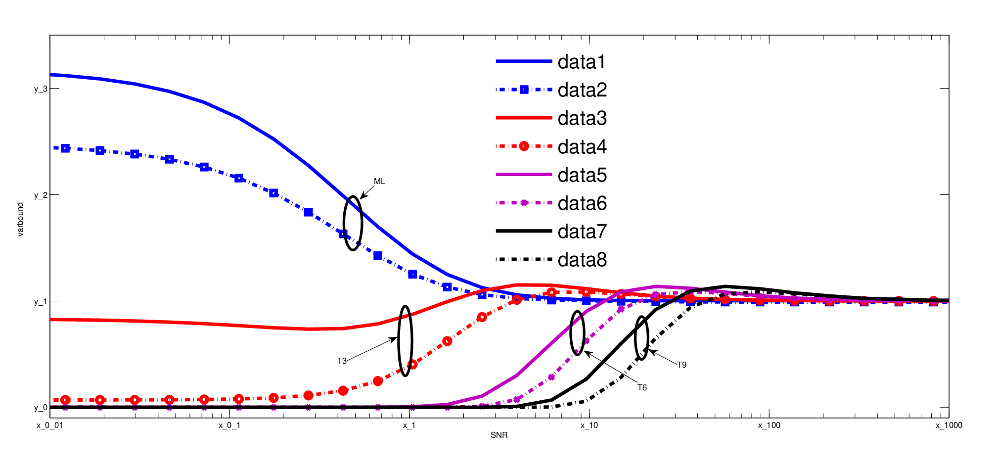
For a numerical evaluation, we considered the SDCM with $N\!\hskip-0.56905pt=\!5$, $S\!=\!1$, $\sigma^{2}\!=\!1$, and $\mathbf{C}_{k}\!=\hskip-0.56905pt\mathbf{e}_{k}\mathbf{e}_{k}^{T}$. We generated parameter vectors $\mathbf{x}_{0}$ with $j_{0}\!=\!1$ and different $\xi_{0}$. In Fig. 1, we show the variance at $\mathbf{x}_{0}$, $v(\hat{\mathbf{x}}(\cdot),\mathbf{x}_{0})\!=\!\sum_{k=1}^{N}v(\hat{x}_{k}(\cdot),\mathbf{x}_{0})$ (computed by means of numerical integration), for the HT estimator using various choices of $\tau$ and for the ML estimator. The variance is plotted versus $\mbox{SNR}=\xi(\mathbf{x}_{0})/\sigma^{2}\hskip-0.56905pt\hskip-0.56905pt=\xi_{0}/\sigma^{2}\hskip-0.56905pt\hskip-0.56905pt$. Along with each variance curve, we display a corresponding lower bound that was calculated by evaluating (21) for each $k$, using for $\gamma_{k}(\mathbf{x})$ the mean function of the respective estimator (HT or ML), and summing over all $k$. (The mean functions of the HT and ML estimators were computed by means of numerical integration.) In evaluating (21), we used partial derivatives of order at most $1$ in (17), and we chose for the evaluation of the lower bound $L\!=\!2$, $\mathcal{K}\!=\hskip-0.56905pt\{k\}$, $\mathbf{p}_{1}\!=\!\mathbf{0}$, and $\mathbf{p}_{2}\!=\hskip-0.56905pt\mathbf{e}_{k}$. In Fig. 1, all variances and bounds are normalized by $2\hskip 0.56905pt(\xi_{0}\hskip-0.56905pt+\hskip-0.56905pt\sigma^{2})^{2}$, which is the variance of the oracle estimator knowing $j_{0}$.

It can be seen from Fig. 1 that in the high-SNR regime, for both estimators, the gap between the variance and the corresponding lower bound is quite small. This indicates that the performance of both estimators is nearly optimal. However, in the low-SNR regime, the variances of the estimators tend to be significantly higher than the bounds. This means that there may be estimators with the same bias and mean function as that of the HT or ML estimator but a lower variance. However, the actual existence of such estimators is not shown by our analysis.

We considered estimation of (a function of) a sparse vector $\mathbf{x}$ that determines the covariance matrix of a Gaussian random vector via a parametric covariance model. Using RKHS theory, we derived lower bounds on the estimator variance for a prescribed bias and mean function. For the important special case of unbiased estimators of $\mathbf{x}$, we found that the transition of our bounds from low to high SNR is significantly slower than that of analogous bounds for the sparse linear model [6]. This suggests that the prior information of sparsity is not as helpful as for the sparse linear model. Numerical results showed that for low SNR, the variance of two standard estimators (hard-thresholding estimator and maximum likelihood estimator) is significantly higher than our bounds. Hence, there might exist estimators that have the same bias and mean function as these standard estimators but a smaller variance.

References

• [1] P. Flandrin, Time-Frequency/Time-Scale Analysis. San Diego (CA): Academic Press, 1999.
• [2] F. Hlawatsch, Time-Frequency Analysis and Synthesis of Linear Signal Spaces: Time-Frequency Filters, Signal Detection and Estimation, and Range-Doppler Estimation. Boston (MA): Kluwer, 1998.
• [3] S. Haykin, “Cognitive radio: Brain-empowered wireless communication,” IEEE J. Sel. Areas Comm., vol. 23, pp. 201–220, Feb. 2005.
• [4] E. Parzen, “Statistical inference on time series by Hilbert space methods, I.” Appl. Math. Stat. Lab., Stanford University, Stanford, CA, Tech. Rep. 23, Jan. 1959.
• [5] D. D. Duttweiler and T. Kailath, “RKHS approach to detection and estimation problems – Part V: Parameter estimation,” IEEE Trans. Inf. Theory, vol. 19, no. 1, pp. 29–37, Jan. 1973.
• [6] S. Schmutzhard, A. Jung, F. Hlawatsch, Z. Ben-Haim, and Y. C. Eldar, “A lower bound on the estimator variance for the sparse linear model,” in Proc. 44th Asilomar Conf. Signals, Systems, Computers, Pacific Grove, CA, Nov. 2010.
• [7] P. Rütimann and P. Bühlmann, “High dimensional sparse covariance estimation via directed acyclic graphs,” Electron. J. Statist., vol. 3, pp. 1133–1160, 2009.
• [8] Y. Chen, A. Wiesel, Y. C. Eldar, and A. O. Hero III, “Covariance estimation in decomposable Gaussian graphical models,” IEEE Trans. Signal Processing, vol. 58, no. 3, pp. 1482–1492, March 2010.
• [9] N. Aronszajn, “Theory of reproducing kernels,” Trans. Am. Math. Soc., vol. 68, no. 3, pp. 337–404, May 1950.
• [10] M. E. Tipping and C. M. Bishop, “Probabilistic principal component analysis,” J. Roy. Stat. Soc. Ser. B, vol. 61, pp. 611–622, 1999.
• [11] D. L. Donoho and I. M. Johnstone, “Ideal spatial adaptation by wavelet shrinkage,” Biometrika, vol. 81, pp. 425–455, 1994.