Evolution of cosmological perturbations in Bose-Einstein condensate dark matter
Abstract
We consider the global cosmological evolution and the evolution of the density contrast in the Bose-Einstein condensate dark matter model, in the framework of a Post-Newtonian cosmological approach. In the Bose-Einstein model, dark matter can be described as a non-relativistic, Newtonian gravitational condensate, whose density and pressure are related by a barotropic equation of state. For a condensate with quartic non-linearity, the equation of state is polytropic with index .The basic equation describing the evolution of the perturbations of the Bose-Einstein condensate is obtained, and its solution is studied by using both analytical and numerical methods. The global cosmological evolution as well as the evolution of the perturbations of the condensate dark matter shows significant differences with respect to the pressureless dark matter model, considered in the framework of standard cosmology. Therefore the presence of condensate dark matter could have modified drastically the cosmological evolution of the early universe, as well as the large scale structure formation process.
Keywords:
cosmology: theory: dark matter: large-scale structure of Universe – instabilities–equation of state1 Introduction
Cosmological observations provide compelling evidence that about 95% of the content of the Universe resides in two unknown forms of energy that we call dark matter and dark energy: the first residing in bound objects as non-luminous matter (Persic et al., 1996; Boriello and Salucci, 2001; Binney & Tremaine, 2008), the latter in the form of a zero-point energy that pervades the whole Universe (Peebles & Ratra, 2003; Padmanabhan, 2003). The dark matter is thought to be composed of cold neutral weakly interacting massive particles, beyond those existing in the Standard Model of Particle Physics, and not yet detected in accelerators or in dedicated direct and indirect searches. There are many possible candidates for dark matter, the most popular ones being the axions and the weakly interacting massive particles (WIMP) (for a review of the particle physics aspects of dark matter see Overduin & Wesson (2004)). Their interaction cross section with normal baryonic matter, while extremely small, are expected to be non-zero and we may expect to detect them directly. It has also been suggested that the dark matter in the Universe might be composed of superheavy particles, with mass GeV (Chung et al., 1998; Chung et al., 2005; Kolb et al., 2007; Chuzhoy & Kolb, 2009). But observational results show the dark matter can be composed of superheavy particles only if these interact weakly with normal matter or if their mass is above GeV (Albuquerque & Baudis, 2003). Scalar fields or other long range coherent fields coupled to gravity have also intensively been used to model galactic dark matter (Lee & Koh, 1996; Nucamendi et al., 2000; Matos & Guzman, 2001; Mielke & Schunk, 2002; Arbey et al., 2003; Fuchs & Mielke, 2004; Hernández et al., 2004; Giannios, 2005; Khlopov et al., 2005; Bernal & Guzman, 2006; Arbey, 2006; Arbey, 2008; Briscese, 2011). Alternative theoretical models to explain the galactic rotation curves have also been elaborated recently (Milgrom, 1983; Mannheim, 1993; Bekenstein, 2004; Mak & Harko, 2004; Brownstein & Moffat, 2006; Harko & Cheng, 2006; Bertolami et al., 2007; Boehmer & Harko, 2007; Boehmer et al., 2008a; Boehmer et al., 2008b; Capozziello et al., 2009).
In order to explain the recent observational data, the CDM ( Cold Dark Matter) model was developed (Peebles & Ratra, 2003; Padmanabhan, 2003). The CDM model successfully describes the accelerated expansion of the Universe, the observed temperature fluctuations in the cosmic microwave background radiation, the large scale matter distribution, and the main aspects of the formation and the evolution of virialized cosmological objects.
Despite these important achievements, at galactic scales kpc, the CDM model meets with severe difficulties in explaining the observed distribution of the invisible matter around the luminous one. In fact, -body simulations, performed in this scenario, predict that bound halos surrounding galaxies must have very characteristic density profiles that feature a well pronounced central cusp, (Navarro et al., 1997), where is a scale radius and is a characteristic density. On the observational side, high-resolution rotation curves show, instead, that the actual distribution of dark matter is much shallower than the above, and it presents a nearly constant density core: (Burkert, 1995), where is the core radius and is the central density.
At very low temperatures, all particles in a dilute Bose gas condense to the same quantum ground state, forming a Bose-Einstein Condensate (BEC), i.e., a sharp peak over a broader distribution in both coordinates and momentum space. A coherent state develops when the particle density is enough high, or the temperature is sufficiently low. The Bose-Einstein condensation process was first observed experimentally in 1995 in dilute alkali gases, such as vapors of rubidium and sodium, confined in a magnetic trap, and cooled to very low temperatures. A sharp peak in the velocity distribution was observed below a critical temperature, indicating that condensation has occurred, with the alkali atoms condensed in the same ground state and showing a narrow peak in the momentum space and in the coordinate space (Anderson et al., 1995; Bradley et al, 1995; Davis et al., 1995). Quantum degenerate gases have been created by a combination of laser and evaporative cooling techniques, opening several new lines of research, at the border of atomic, statistical and condensed matter physics (Dalfovo et al., 1999; Cornell & Wieman, 2002; Ketterle, 2002; Pitaevskii & Stringari, 2003; Duine & Stoof, 2004; Chen et al., 2005; Pethick & Smith, 2008).
The possibility that dark matter could be in the form of a Bose-Einstein condensate was considered in Sin (1994) and Ji & Sin (1994). The condensate was described by the non-relativistic Gross-Pitaevskii equation, and its solution was obtained numerically. An alternative approach was developed in Boehmer & Harko (2007). By introducing the Madelung representation of the wave function, the dynamics of the system can be formulated in terms of the continuity equation and of the hydrodynamic Euler equations. Hence dark matter can be described as a non-relativistic, Newtonian Bose-Einstein gravitational condensate gas, whose density and pressure are related by a barotropic equation of state. In the case of a condensate with quartic non-linearity, the equation of state is polytropic with index . To test the validity of the model the Newtonian tangential velocity equation of the model was fitted with a sample of rotation curves of low surface brightness and dwarf galaxies, respectively. A very good agreement was found between the theoretical rotation curves and the observational data for the low surface brightness galaxies. Therefore dark matter halos can be described as an assembly of light individual bosons that acquire a repulsive interaction by occupying the same ground energy state. That prevents gravity from forming the central density cusps. The condensate particle is light enough to naturally form condensates of very small masses that later may coalesce, forming the structures of the Universe in a similar way than the hierarchical clustering of the bottom-up CDM picture. Then, at large scales, BEC perfectly mimic an ensemble of cold particles, while at small scales quantum mechanics drives the mass distribution. Different properties of the Bose-Einstein condensate dark matter halos, like the effects of the rotation and of the vortices, as well as the cosmological effects of the condensation were also investigated (Ferrer & Grifols, 2004; Fukuyama et al., 2008; Fukuyama & Morikawa, 2009; Rindler-Daller & Shapiro, 2009; Sikivie & Yang, 2009; Lee, 2009; Brook & Coles, 2009; Kain & Ling, 2010; Lee & Lim, 2010).
It is the purpose of the present paper to study the global cosmological dynamics of gravitationally self-bound Bose-Einstein dark matter condensates, and the evolution of the small cosmological perturbations in the condensate. The equations of motion of the condensate dark matter are obtained in a Post-Newtonian approximation by using the conservation of the general relativistic energy-momentum tensor, and considering the small velocity limit. The cosmological dynamics of the Bose-Einstein condensate is also studied. The exact solution of the Friedmann equations is obtained, and it is compared with the standard Einstein-de Sitter cosmological model. In order to study the evolution of the small cosmological perturbations the equation describing the Newtonian perturbations with pressure is obtained in a general form, by also taking into account a term which was neglected in the previous studies of this problem (McCrea, 1951; Harrison, 1965; Lima et al., 1997; Reis, 2003; Abramo et al., 2007; Pace et al., 2010). The equation of the density contrast for the Bose-Einstein condensate is investigated by using both analytical and numerical methods. The presence of the condensate dark matter significantly modifies the cosmological dynamics of the Universe, as well as the large scale structure formation.
The present paper is organized as follows. The basic properties of the Bose-Einstein condensate dark matter halos are reviewed in Section 2. The Post-Newtonian hydrodynamical equations of motion for a perfect fluid with pressure are derived in Section 3. The cosmological dynamics of the Bose-Einstein condensate dark matter is considered in Section 4. The equation describing the small cosmological perturbations of a fluid with pressure are derived in Section 5. The evolution of the small cosmological perturbations in a Bose-Einstein condensate is considered in Section 6. We discuss and conclude our results in Section 7.
2 Dark matter as a Bose-Einstein condensate
In a quantum system of interacting condensed bosons most of the bosons lie in the same single-particle quantum state. For a system consisting of a large number of particles, the calculation of the ground state of the system with the direct use of the Hamiltonian is impracticable, due to the high computational cost. However, the use of some approximate methods can lead to a significant simplification of the formalism. One such approach is the mean field description of the condensate, which is based on the idea of separating out the condensate contribution to the bosonic field operator. We also assume that in a medium composed of scalar particles with non-zero mass, when the medium makes a transition to a Bose-Einstein condensed phase, the range of Van der Waals-type scalar mediated interactions among particles becomes infinite.
2.1 The Gross-Pitaevskii equation
The many-body Hamiltonian describing the interacting bosons confined by an external potential is given, in the second quantization, by
| (1) |
where and are the boson field operators that annihilate and create a particle at the position , respectively, and is the two-body interatomic potential (Dalfovo et al., 1999; Chen et al., 2005). is the potential associated to the rotation of the condensate.
The use of some approximate methods can lead to a significant simplification of the formalism. One such approach is the mean field description of the condensate, which is based on the idea of separating out the condensate contribution to the bosonic field operator. For a uniform gas in a volume , BEC occurs in the single particle state , having zero momentum. The field operator can be decomposed then in the form . By treating the operator as a small perturbation, one can develop the first order theory for the excitations of the interacting Bose gases (Dalfovo et al., 1999; Barcelo et al., 2001).
In the general case of a non-uniform and time-dependent configuration the field operator in the Heisenberg representation is given by , where , also called the condensate wave function, is the expectation value of the field operator, . It is a classical field, and its absolute value fixes the number density of the condensate through . The normalization condition is , where is the total number of particles in the condensate.
The equation of motion for the condensate wave function is given by the Heisenberg equation corresponding to the many-body Hamiltonian given by Eq. (1),
| (2) |
The zeroth-order approximation to the Heisenberg equation is obtained by replacing with the condensate wave function . In the integral containing the particle-particle interaction this replacement is in general a poor approximation for short distances. However, in a dilute and cold gas, only binary collisions at low energy are relevant, and these collisions are characterized by a single parameter, the -wave scattering length , independently of the details of the two-body potential. Therefore, one can replace with an effective interaction , where the coupling constant is related to the scattering length through , where is the mass of the condensed particles. With the use of the effective potential the integral in the bracket of Eq. (2) gives , and the resulting equation is the Schrodinger equation with a quartic nonlinear term (Chen et al., 2005). However, in order to obtain a more general description of the Bose-Einstein condensate stars, we shall assume an arbitrary non-linear term (Barcelo et al., 2001).
Therefore the generalized Gross-Pitaevskii equation describing a gravitationally trapped rotating Bose-Einstein condensate is given by
| (3) | |||||
where we denoted . As for , we assume that it is the gravitational potential , , and it satisfies the Poisson equation
| (4) |
where is the mass density inside the Bose-Einstein condensate.
2.2 The hydrodynamical representation
The physical properties of a Bose-Einstein condensate described by the generalized Gross-Pitaevskii equation given by Eq. (3) can be understood much easily by using the so-called Madelung representation of the wave function (Dalfovo et al., 1999), which consist in writing in the form
| (5) |
where the function has the dimensions of an action. By substituting the above expression of into Eq. (3), it decouples into a system of two differential equations for the real functions and , given by
| (6) |
| (7) |
where we have introduced the quantum potential
| (8) |
and the velocity of the quantum fluid
| (9) |
respectively, and we have denoted
| (10) |
From its definition it follows that the velocity field is irrotational, satisfying the condition . Therefore the equations of motion of the gravitational ideal Bose-Einstein condensate take the form of the equation of continuity and of the hydrodynamic Euler equations. The Bose-Einstein gravitational condensate can be described as a gas whose density and pressure are related by a barotropic equation of state (Pethick & Smith, 2008). The explicit form of this equation depends on the form of the non-linearity term .
When the number of particles in the gravitationally bounded Bose-Einstein condensate becomes large enough, the quantum pressure term makes a significant contribution only near the boundary of the condensate. Hence it is much smaller than the non-linear interaction term. Thus the quantum stress term in the equation of motion of the condensate can be neglected. This is the Thomas-Fermi approximation, which has been extensively used for the study of the Bose-Einstein condensates (Dalfovo et al., 1999; Chen et al., 2005). As the number of particles in the condensate becomes infinite, the Thomas-Fermi approximation becomes exact. This approximation also corresponds to the classical limit of the theory (it corresponds to neglecting all terms with powers of , or, equivalently, to the regime of strong repulsive interactions among particles). From a mathematical point of view, the Thomas-Fermi approximation corresponds to neglecting in the equation of motion all terms containing and .
In the standard approach to the Bose-Einstein condensates, the non-linearity term is given by
| (11) |
where (Dalfovo et al., 1999; Chen et al., 2005). The corresponding equation of state of the condensate is
| (12) |
with
| (13) | |||||
Therefore the equation of state of the Bose-Einstein condensate with quartic non-linearity is a polytrope with index . However, in the case of low dimensional systems Kolomeisky et al. (2000) have shown that in many experimentally interesting cases the nonlinearity will be cubic, or even logarithmic, in . The strong interaction assumption is valid only if the interaction energy per particle is much bigger than the ground-state energy (due to the zero-point motion) per particle. This is the case for condensates in the dilute limit below two dimensions. But as space dimensionality decreases, it becomes increasingly harder for the repulsive particles to avoid collisions. Thus the correlations between particle dominate, and the quartic nonlinearity should be replaced by a more general, power-law term (Kolomeisky et al., 2000). Hence more general models, with the non-linearity term of the form , where constant and constant, can also be considered. In this case the equation of state of the gravitational Bose-Einstein condensate is the standard polytropic equation of state, , and the structure of the static gravitationally bounded Bose-Einstein condensate is described by the Lane-Emden equation, , where and is a dimensionless variable defined by , where is the central density of the condensate. The dimensionless radial coordinate is defined by the relation . Hence Bose-Einstein condensate dark matter can generally be described as fluid satisfying a polytropic equation of state of index .
In the following we will consider only the case of the condensate with quartic non-linearity. In this case the physical properties of the condensate are relatively well known from laboratory experiments, and its properties can be described in terms of only two free parameters, the mass of the condensate particle, and the scattering length , respectively.
2.3 Dark matter as a Bose-Einstein condensate
In the case of a static Bose-Einstein condensate, all physical quantities are independent of time. Moreover, in the first approximation we can also neglect the rotation of the condensate, by taking . Therefore the equations describing the static Bose-Einstein condensate in a gravitational field with potential take the form
| (14) |
| (15) |
These equations must be integrated together with the equation of state , and some appropriately chosen boundary conditions. The density distribution of the static gravitationally bounded single component dark matter Bose-Einstein condensate is given by (Boehmer & Harko, 2007)
| (16) |
where and is the central density of the condensate, . The mass profile of the Bose-Einstein condensate galactic halo is
| (17) |
with a boundary radius . At the boundary of the dark matter distribution , giving the condition , which fixes the radius of the condensate dark matter halo as . The tangential velocity of a test particle moving in the condensed dark halo can be represented as (Boehmer & Harko, 2007)
| (18) |
The mass of the particle in the condensate can be obtained from the radius of the dark matter halo in the form (Boehmer & Harko, 2007)
| (19) | |||||
From this equation it follows that is of the order of eV. For fm and kpc, the mass is of the order of meV. For values of of the order of fm, corresponding to the values of observed in terrestrial laboratory experiments, eV. These values are perfectly consistent with the limit eV obtained for the mass of the condensate particle from cosmological considerations (Fukuyama et al., 2008).
3 Post-Newtonian hydrodynamics of the Bose-Einstein condensates
In order to study gravitational effects on the evolution of Bose-Einstein condensate dark halos a full general relativistic treatment is needed. The equations of motion of the condensate are obtained from the conservation of the energy-momentum tensor, , with ; denoting the covariant derivative with respect to the metric , and
| (20) |
where is the four-velocity of the fluid, satisfying the conditions and , respectively. By taking the covariant divergence of we obtain the equation
| (21) |
where a comma denotes the ordinary derivative with respect to the coordinate . By contracting Eq. (21) with , we obtain
| (22) |
In the Newtonian limit of small condensate velocities the four-velocity is given by , where is the three-velocity of the condensate. The four-divergence of the four-velocity is given by , where is the determinant of the metric tensor. In the Newtonian limit we assume that , that is, the deviations from the Minkowski type geometry are small. Under these assumptions, from Eq. (22) we obtain the equation of continuity of the Bose-Einstein condensate as
| (23) |
where all differential operations are considered with respect to the physical coordinate . By contracting Eq. (21) with the projection operator , with the property , we obtain the relativistic Euler equation of motion as
| (24) |
In the Newtonian approximation the generalized Euler equation of motion becomes
| (25) |
The gravitational potential satisfies the generalized Poisson equation,
| (26) |
Eqs. (23), (25) and (26) represent the basic equations describing the dynamics of a gravitationally bounded Bose-Einstein condensate in the first Post-Newtonian approximation (McCrea, 1951; Harrison, 1965; Lima et al., 1997; Reis, 2003; Abramo et al., 2007; Pace et al., 2010).
4 Cosmological dynamics of Bose-Einstein condensates
The Bose-Einstein condensation takes place when particles (bosons) become correlated with each other. This happens when their wavelengths overlap, that is, the thermal wavelength is greater than the mean inter-particles distance , . The critical temperature for the condensation to take place is (Dalfovo et al., 1999). On the other hand, cosmic evolution has the same temperature dependence, since in an adiabatic expansion process the density of a matter dominated Universe evolves as (Fukuyama & Morikawa, 2009). Therefore, if the boson temperature is equal, for example, to the radiation temperature at , the critical temperature for the Bose-Einstein condensation is at present (Fukuyama & Morikawa, 2009). Since the matter temperature varies as , where is the scale factor of the Universe, it follows that during an adiabatic evolution the ratio of the photon temperature and of the matter temperature evolves as . Using for the present day energy density of the Universe the value g/cm3, BEC takes place provided that the boson mass satisfies the restriction eV (Fukuyama et al., 2008). Thus, once the temperature of the boson is less than the critical temperature, BEC can always take place at some moment during the cosmological evolution of the Universe. On the other hand, we expect that the Universe is always under critical temperature, if it is at the present time (Fukuyama & Morikawa, 2009). Another cosmological bound on the mass of the condensate particle can be obtained as eV (Boyanovski et al., 2008), where is the number of internal degrees of freedom of the particle before decoupling, is the number of internal degrees of freedom of the particle at the decoupling, and is the decoupling temperature. In the Bose condensed case , and it follows that the BEC particle should be light, unless it decouples very early on, at high temperature and with a large . Therefore, depending on the relation between the critical and the decoupling temperatures, in order for a BEC light relic to act as cold dark matter, the decoupling scale must be higher than the electroweak scale (Boyanovski et al., 2008).
The set of equations Eqs. (23), (25) and (26) admits a homogeneous and isotropic cosmological background solution with and . In this case the fluid’s velocity is given by
| (27) |
and the evolution of the scale factor is determined by the Friedmann equations,
| (28) |
and
| (29) |
respectively, where we have denoted . The continuity equation Eq. (23) reduces to
| (30) |
In the case of the Bose-Einstein condensates the equation of state is given by , and Eq. (30) can be integrated immediately to obtain
| (31) |
where is an arbitrary constant of integration. By assuming that the present-day density of the Bose-Einstein condensate, , is obtained for a value of the scale factor, we obtain , and the background cosmological density of the condensate can be written as
| (32) |
where we have denoted
| (33) |
The energy density of the Bose-Einstein condensate diverges as . The equation determining the time evolution of the scale factor is given by
| (34) |
where we have denoted
| (35) |
where is the present day density parameter of the Bose-Einstein condensate, is the present day critical density of the Universe, and is the present day value of the Hubble parameter, respectively.
Eq. (34) can be integrated immediately to give the time evolution of the scale factor of the Bose-Einstein condensate as
| (36) |
where is an arbitrary constant of integration. The constant can be determined from the condition when , thus obtaining . Therefore the time evolution of the scale factor is described by the equation
| (37) | |||||
where we denoted .
In the case of the standard dark matter models, dark matter is assumed to be a pressureless fluid, and the background cosmological evolution is described by the Einstein-de Sitter model, with the scale factor given by , where is the present day density parameter of the dark matter, and we have assumed that . In the following for the Hubble constant we adopt the value (Hinshaw et al., 2009), giving for the critical density a value of . The constant can be represented as
| (38) |
while for we obtain
| (39) |
The two parameters and , describing the global properties of the condensate, are related by the relation .
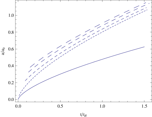
By assuming that the entire existing dark matter is in the form of a Bose-Einstein condensate, it follows that (Hinshaw et al., 2009). By assuming that meV and fm, we obtain , while . For these values of the physical parameters of the condensate the energy density of the dark matter diverges for . The time evolution of the scale factor for the Bose-Einstein condensate dark matter, for different values of the parameters and , and for the pressureless dark matter, are represented in Fig. 1, respectively. The cosmological dynamics of the condensate dark matter shows significant differences as compared to the standard pressureless dark matter model, with the condensate expanding much faster than the cosmological fluid of the standard CDM model, with the speed of expansion increasing with increasing .
In the case of a Universe filled with dark energy, radiation, baryonic matter with negligible pressure, and Bose-Einstein condensed dark matter, respectively, the time evolution of the scale factor is given by
| (40) |
where , , and are the present day values of the density parameters of the baryonic matter, radiation, and dark energy, respectively. For , , and we adopt the numerical values , and (Hinshaw et al., 2009). In the case of the standard CDM cosmological, model the Friedmann equation describing the evolution of the Universe containing baryons, pressureless dark matter, radiation, and dark energy, is given by
| (41) |
The time evolutions of the scale factors for Universes containing BEC dark matter and standard pressureless dark matter are represented, for different values of the BEC parameter , in Fig. 2. The presence of the condensate dark matter changes the global cosmological dynamics of the Universe, and the magnitude of the changes increases with the increase of the BEC parameter .

5 Cosmological perturbations of an expanding Bose-Einstein condensate
In the gravitationally bounded Bose-Einstein condensate we assume small perturbations of the physical quantities around the homogeneous background of the form
| (42) |
| (43) |
| (44) |
| (45) |
In Eqs. (42)-(45) the index denotes the background quantities. Substituting these equations into the continuity equation Eq. (23) we obtain
| (46) |
The variation of the equation of motion Eq. (25) gives
| (47) |
The Poisson equations for the perturbation of the gravitational potential, obtained by perturbing Eq. (26), can be written as
| (48) |
In order to describe the cosmological evolution we make a change to the comoving coordinate system, so that , , and
| (49) |
respectively. To simplify the notation we define the parameters and , respectively, which generally are functions of the time only. We also introduce the density contrast as . The time derivative of the background pressure is related to the speed of sound of the background condensate by the relation
| (50) |
Therefore the perturbation equations Eqs. (43) - (45) can be written as
| (51) |
| (52) |
| (53) |
In the following we denote
| (54) |
and
| (55) |
respectively. is related to the time derivative of by the relation
| (56) |
By taking the time derivative of Eq. (51), the divergence of Eq. (52), by eliminating by using the perturbed equation of continuity, and with the use of Eq. (53), we obtain the equation giving the evolution of the density contrast as
| (57) |
Changing the independent variable from the time to the scale factor using the relations and , we obtain the evolution equation in the form
| (58) |
Eq. (57) is different from the perturbation equation obtained in the Newtonian cosmology with pressure by Lima et al. (1997), Reis (2003), and Abramo et al. (2007), respectively. The reason is that we have included in our analysis the term , which was neglected in the previous studies. This term generates the new term in the left hand side of Eq. (52), which modifies the final perturbation equation. On the other hand, in the present approach the term was neglected.
In order to numerically integrate Eq. (57) or Eq. (58) we have to chose some physically appropriate initial conditions. In the current standard model for structure formation in the Universe, it is supposed that quantum fluctuations were generated during an initial period of inflation. These fluctuations inflated up to super-horizon scales, producing a near scale-invariant, and near Gaussian, set of primordial potential fluctuations. At the end of inflation, the Universe is reheated, and particles and radiation are produced. In this hot early phase, cold thermal relics (dark matter) are also formed (Peebles & Ratra, 2003; Padmanabhan, 2003). Dark matter particles interact gravitationally, and possibly through the weak interaction. Therefore in order to obtain some physically realistic initial conditions for the state of the Universe during large scale structure formation, one needs to evolve cosmological perturbations, starting from initial conditions, deep inside the radiation epoch, and far outside the Hubble radius. Initial conditions for photons, neutrinos, cold dark matter and baryons have been obtained, in the framework of the standard CDM cosmological model, in both the synchronous and Newtonian gauges, by Ma & Bertschinger (1995). In the conventional method, the power spectrum of the matter fluctuations in the Universe is computed by numerically solving the Boltzmann equation. The power spectrum is usually obtained in the linear theory, and then extrapolated to the present epoch. In the standard cosmology, in first-order Eulerian perturbation theory, all modes evolve independently, and the power spectrum can be scaled back to the initial epoch via the growth function (Ma & Bertschinger, 1995). Moreover, the effect of the dark matter pressure is generally ignored in the conventional methods of generating initial conditions. On the other hand, the exact moment in the history of the Universe when the Bose-Einstein condensation occurred is not known. That’s why obtaining the rigorous and physically well motivated initial conditions for the density contrast and for its derivative for BEC dark matter requires the full investigation of the cosmological dynamics from the reheating era, by taking into account the dark matter condensation and pressure effects.
6 Cosmological evolution of small perturbations in a Bose-Einstein condensate
By taking into account the equation of state of the Bose-Einstein condensate, we immediately obtain , and , respectively. The conditions and imposes the constraint , and in the following we will consider that the model considered in the present paper is valid only for this range of values of the scale factor. Hence for the time evolution of the linear density perturbations of the Bose-Einstein condensate dark matter we obtain successively
| (59) |
and
| (60) |
respectively, where we have denoted . In the limit of large , when , , and Eq. (60) becomes
| (61) |
with the solution
| (62) |
where and are arbitrary constants of integration. Hence in the limit of a pressureless fluid we recover the standard general relativistic result. In the limit of small , so that , we can approximate Eq. (60) as
| (63) |
with the solution
| (64) |
where and are two arbitrary constants of integration.
By introducing as a new independent variable, Eq. (60) can be written as
| (65) |
By representing the density contrast as , it follows that the new function satisfies the equation
| (66) |
Therefore the general solution of Eq. (65) can be obtained as
where is the hypergeometric function, , , and and are arbitrary constants of integration. The constants of integration can be determined from the initial conditions. When , , and and , where we have denoted and , respectively. In the limit of large , , and the density contrast can be approximated as
Near the initial state , the density contrast can be approximated as
| (69) | |||||
Since Eq. (60) is valid only in the linear regime of small perturbations, we assume that the initial value of the perturbation, , occurring for a value of the scale factor, satisfies the condition . Since the equation describing the perturbations is a second order differential equation, two initial values have to be given, one for the initial perturbation , and one for the initial rate of evolution of the perturbation, . We consider two cases, namely, the case of a perturbation with an initial low evolution rate, of the order of , and the case of a perturbation with a very high initial evolution rate, , respectively. The comparison between the evolution of the evolution of the linear perturbations for pressureless dark matter in an expanding Einstein - de Sitter cosmological background, and the evolution of the density perturbations in a Bose-Einstein condensate dark matter dominated Universe is presented in Figs. 3 and 4, respectively.
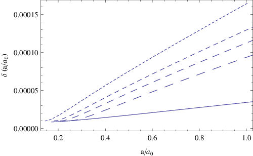
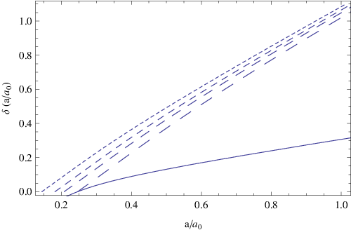
As one can see from Figs. 3 and 4, for all initial conditions, in the case of the Bose-Einstein, for a given , the amplitude of the density contrast is higher as compared to the case of the standard dark matter model. The condensate enters more rapidly in the non-linear phase () than the pressureless dark matter. Thus the presence of the Bose-Einstein condensate dark matter can significantly accelerate the process of cosmic structure formation.
7 Discussions and final remarks
In the present paper we have considered the global cosmological evolution and the evolution of the small cosmological perturbation in a Bose-Einstein dark matter condensate. The basic equation describing the evolution of the small perturbations in the Post-Newtonian regime was obtained, and its solutions have been studied by using both analytical and numerical methods. The evolution of the density perturbations of the condensate has been compared to the evolution of the small cosmological perturbations in a pressureless fluid evolving in an Einstein-de Sitter cosmological background. Depending on the numerical values of the physical parameters describing the condensate (the mass of the particle and the scattering length, respectively), significant differences could appear in the evolution of the Bose-Einstein condensate dark matter halos, as compared to the standard pressureless dark matter models. These differences appear at both the level of the global cosmological evolution, and of the behavior of the small perturbations in the dark matter fluid, and they could have fundamental implications for the formation of the large-scale structure in the Universe.
One of the most important problems present day cosmology faces is the problem of the galaxy formation. To explain galaxy formation the evolution of the linear density and temperature perturbations in a Universe with dark matter, baryons, and radiation must be computed. For pressureless dark matter the evolution of the perturbations of all cosmic components, from cosmic recombination until the epoch of the first galaxies, was obtained in Naoz & Barkana (2005). The evolution of sub-horizon linear perturbations can be described by two coupled, second-order differential equations, with the pressureless dark matter interacting gravitationally with itself, and with the baryons, while the baryons experience both gravity and pressure. Starting from very low values on sub-horizon scales, the baryon density perturbations gradually approach those in the dark matter, and the temperature perturbations approach the value expected for an adiabatic gas. The presence of the baryons does not modify significantly the evolution of the dark matter perturbations. By including the effect of the BEC pressure in the perturbations equations for baryons and dark matter, a more general (and realistic) description of the galaxy formation process can be obtained. The presence of the BEC modifies the dynamical evolution of the baryons, and the growth of linear perturbations, which provide the initial conditions for the formation of galaxies. In the BEC condensate model the dark matter perturbations grow more rapidly than in the standard cosmology, and therefore this could lead to a much faster growth rate of the baryonic perturbations, accelerating the galaxy formation process.
A major recent experimental advance in the study of the Bose-Einstein condensation processes was the observation of the collapse and subsequent explosion of the condensates (Rybin et al., 2004). A dynamical study of an attractive 85Rb BEC in an axially symmetric trap was done, where the interatomic interaction was manipulated by changing the external magnetic field, thus exploiting a nearby Feshbach resonance. In the vicinity of a Feshbach resonance the atomic scattering length a can be varied over a huge range, by adjusting an external magnetic field. Consequently, the sign of the scattering length is changed, thus transforming a repulsive condensate of 85Rb atoms into an attractive one, which naturally evolves into a collapsing and exploding condensate. From a simple physical point of view the collapse of the Bose-Einstein condensates can be described as follows. When the number of particles becomes sufficiently large, so that , where is a critical number, the attractive inter-particle energy overcomes the quantum pressure, and the condensate implodes. In the course of the implosion stage, the density of particles increases in the small vicinity of the trap center. When it approaches a certain critical value, a fraction of the particles gets expelled. In a time period of an order of few milliseconds, the condensate again stabilizes. There are two observable components at the final stage of the collapse: remnant and burst particles. The remnant particles are those which remain in the condensate. The burst particles have an energy much larger than that of the condensed particles. There is also a fraction of particles, which is not observable. This fraction is usually referred to as the missing particles.
The scattering length is defined as the zero-energy limit of the scattering amplitude (Dalfovo et al., 1999). Depending on the spin dependence of the underlying particle interaction, the scattering length may in general be also spin dependent. The spin independent part of the quantity is referred to as the coherent scattering length . The scattering lengths can be obtained for some systems in the laboratory, but for dark matter it is unknown. Another essential parameter is the mass of the condensate particle, which, due to the lack of information about the physical nature of the dark matter, is a free parameter, which must be constrained by observations. Due to the lack of any physical information about the numerical values of these two fundamental parameters, in the numerical estimations performed in the present paper we have given different numerical values to a combination of these two basic quantities.
Since Bose-Einstein condensates are less stable with respect to perturbations than usual non-condensate matter, we expect that in such a condensate evolution of the perturbations and the subsequent collapse could take place much faster than in the usual non-condensed matter. This would strongly affect the formation of the large scale structure in the early Universe. In this paper we have provided some basic theoretical tools necessary for the in depth comparison of the predictions of the condensate model and of the observational results.
Acknowledgments
I would like to thank to the anonymous referee for comments and suggestions that helped me to considerably improve the manuscript. The work described in this paper was fully supported by a grant from the Research Grants Council of the Hong Kong Special Administrative Region, China.
References
- Abramo et al. (2007) Abramo L. R., Batista R. C., Liberato L., Rosenfeld R., 2007, J. Cosmol. Astropart. Phys., 11, 12
- Albuquerque & Baudis (2003) Albuquerque I. F. M., Baudis L., 2003, Phys. Rev. Lett., 90, 221301
- Anderson et al. (1995) Anderson M. H., Ensher J. R., Matthews M. R., Wieman C. E., Cornell E. A., 1995, Science, 269, 198
- Arbey et al. (2003) Arbey, A., Lesgourgues, J., Salati, P., 2003, Phys. Rev. D, 68, 023511
- Arbey (2006) Arbey, A., 2006, Phys. Rev. D, 74, 043516
- Arbey (2008) Arbey, A., 2008, The Open Astronomy Journal, 1, 27
- Barcelo et al. (2001) Barcelo C., Liberati L., Visser M., 2001, Class. Quant. Grav., 18, 1137
- Bekenstein (2004) Bekenstein J. D., 2004, Phys. Rev. D, 70, 083509
- Bernal & Guzman (2006) Bernal A., Siddhartha Guzman F., 2006, Phys. Rev. D, 74, 063504
- Bertolami et al. (2007) Bertolami O., Boehmer C. G., Harko T., Lobo F. S. N., 2007, Phys. Rev. D, 75, 104016
- Binney & Tremaine (2008) Binney J., Tremaine S., 2008, Galactic dynamics, Princeton, N.J.; Woodstock: Princeton University Press
- Boriello and Salucci (2001) Boriello A., Salucci P., 2001, Mon. Not. R. Astron. Soc. 323, 285
- Boehmer & Harko (2007) Boehmer C. G., Harko T., 2007, Mon. Not. R. Astron. Soc., 379, 393
- Boehmer & Harko (2007) Boehmer C. G., Harko T., 2007, J. Cosmol. Astropart. Phys., 06, 025
- Boehmer et al. (2008a) Boehmer C. G., Harko T., Lobo F. S. N., 2008a, Astropart. Phys., 29, 386
- Boehmer et al. (2008b) Boehmer C. G., Harko T., Lobo F. S. N., 2008b, J. Cosmol. Astropart. Phys., 0803, 024
- Boyanovski et al. (2008) Boyanovsky D., de Vega H. J., Sanchez N., 2008, Phys. Rev. D, 77, 043518
- Bradley et al (1995) Bradley C. C., Sackett C. A., Tollett J. J., Hulet R. G., 1995, Phys. Rev. Lett., 75, 1687
- Briscese (2011) Briscese, F., 2011, Phys. Lett. B, 696, 315
- Brook & Coles (2009) Brook, M. N., Coles, P., 2009, arXiv:0902.0605
- Brownstein & Moffat (2006) Brownstein J. R., Moffat J. W., 2006, Mon. Not. R. Astron. Soc., 367, 527
- Burkert (1995) Burkert A., 1995, Astrophys. J. Letters, 447, L25
- Capozziello et al. (2009) Capozziello S., Piedipalumbo E., Rubano C., Scudellaro P., 2009, Astron. Astrophys., 505, 21
- Chen et al. (2005) Chen Q., Stajic J., Tan S., Levin K., 2005, Phys. Rept., 412, 1
- Chung et al. (1998) Chung, D. J. H., Kolb, E. W., Riotto, A., 1998, Phys. Rev. Lett., 81, 4048
- Chung et al. (2005) Chung, D. J. H., Kolb, E. W., Riotto, A., Senatore, L., 2005, Phys. Rev. D, 72, 023511
- Chuzhoy & Kolb (2009) Chuzhoy, L., Kolb, E, W., 2009, JCAP, 0907, 014
- Cornell & Wieman (2002) Cornell E. A., Wieman C. E., 2002, Rev. Mod. Phys., 74, 875
- Dalfovo et al. (1999) Dalfovo F., Giorgini S., Pitaevskii L. P., Stringari S., 1999, Rev. Mod. Phys., 71, 463
- Davis et al. (1995) Davis K. B., Mewes M. O., Andrews M. R., van Drutten N. J., Durfee D. S., Kurn D. M., Ketterle W., 1995, Phys. Rev. Lett., 75, 3969
- Duine & Stoof (2004) Duine R. A., Stoof H. T. C., 2004, Phys. Repts., 396, 115
- Ferrer & Grifols (2004) Ferrer, F., Grifols, J. A., 2004, J. Cosmol. Astropart. Phys., 12, 012
- Fuchs & Mielke (2004) Fuchs B., Mielke E. W., 2004, Month. Not. R. Acad. Sci., 350, 707
- Fukuyama et al. (2008) Fukuyama, T., Morikawa, M., Tatekawa, T., 2008, JCAP, 06, 033
- Fukuyama & Morikawa (2009) Fukuyama, T., Morikawa, M., 2009, Phys. Rev. D, 80, 063520
- Giannios (2005) Giannios D., Phys. Rev. D, 71, 103511
- Harrison (1965) Harrison E. R., 1965, Ann. Phys., 35, 437
- Harko & Cheng (2006) Harko T., Cheng K. S., 2006, Astrophys. J., 636, 8
- Hernández et al. (2004) Hernández X., Matos T., Sussman R. A., Verbin Y., 2004, Phys. Rev. D, 70, 043537
- Hinshaw et al. (2009) Hinshaw G., et al., 2009, The Astrophysical Journal Supplement, 180, 225
- Ji & Sin (1994) Ji S. U., Sin S. J., 1994, Phys. Rev. D, 50, 3655
- Kain & Ling (2010) Kain, B., Ling, H. Y., 2010, Phys. Rev. D, 82, 064042
- Ketterle (2002) Ketterle W., 2002, Rev. Mod. Phys., 74, 1131
- Khlopov et al. (2005) Khlopov, M. Y., Rubin, S. G., Sakharov, A. S., 2005, Astropart. Phys., 23, 265
- Kolb et al. (2007) Kolb, E. W., Starobinsky, A. A., Tkachev, I. I., 2007, JCAP, 0707, 005
- Kolomeisky et al. (2000) Kolomeisky, E. B., Newman, T. J., J Straley, J. P., Qi, X., 2000, Phys. Rev. Lett., 85, 1146
- Lee & Koh (1996) Lee, J.-W., Koh, I.-G., 1996, Phys. Rev. D, 53, 2236
- Lee (2009) Lee, J.-W., 2009, Phys. Lett. B, 681, 118
- Lee & Lim (2010) Lee, J.-W., Lim, S., 2010, J. Cosmol. Astropart. Phys., 01, 007
- Lima et al. (1997) Lima J. A. S., Zanchin V., Brandenberger R., 1997, Mon. Not. R. Astron. Soc., 291, L1
- Naoz & Barkana (2005) Naoz, S., Barkana, R. 2005, Mon. Not. R. Astron. Soc., 362, 1047
- Navarro et al. (1997) Navarro J. F., Frenk C. S., White S. D. M., 1997, Astrophys. J., 490, 493
- Nucamendi et al. (2000) Nucamendi U., Salgado M., Sudarsky D., 2000, Phys. Rev. Lett., 84, 3037
- Ma & Bertschinger (1995) Ma, C.-P., Bertschinger, E., 1995, Astrophys. J., 455, 7
- Mak & Harko (2004) Mak M. K., Harko T., 2004, Phys. Rev. D, 70, 024010
- Mannheim (1993) Mannheim P. D., 1993, Astrophys. J., 419, 150
- Matos & Guzman (2001) Matos T., Guzman F. S., Class. Quant. Grav., 18, 5055
- McCrea (1951) McCrea W. H., 1951, Proc. R. Soc. London A, 206, 562
- Mielke & Schunk (2002) Mielke E. W., Schunk F. E., 2002, Phys. Rev. D, 66, 023503
- Milgrom (1983) Milgrom M., 1983, Astrophys. J., 270, 365
- Overduin & Wesson (2004) Overduin J. M., Wesson P. S., 2004, Phys. Repts. 402, 267
- Pace et al. (2010) Pace F., Waizmann J.-C., Bartelmann M., 2010, Mon. Not. R. Astron. Soc., 406, 1865
- Padmanabhan (2003) Padmanabhan T., 2003, Phys. Repts., 380, 235
- Persic et al. (1996) Persic M., Salucci P., Stel F., 1996, Mon. Not. R. Astron. Soc., 281, 27
- Peebles & Ratra (2003) Peebles P. J. E, Ratra B., 2003, Rev. Mod. Phys. 75, 559
- Pethick & Smith (2008) Pethick C. J., Smith H., 2008, Bose-Einstein condensation in dilute gases, Cambridge, Cambridge University Press
- Pitaevskii & Stringari (2003) Pitaevskii L., Stringari S., 2003, Bose-Einstein condensation, Clarendon Press, Oxford
- Reis (2003) Reis R. R. R., 2003, Phys. Rev. D, 67, 087301
- Rindler-Daller & Shapiro (2009) Rindler-Daller, T., Shapiro, P. R., 2009, Vortices and Angular Momentum in Bose-Einstein-Condensed Cold Dark Matter Halos, to appear in ”New Horizons in Astronomy (Bash Symposium 2009)”, Proceedings of the Astronomical Society of the Pacific, eds. L. Stanford, L. Hao, Y. Mao, J. Green, arXiv:0912.2897
- Rybin et al. (2004) Rybin, A. V., Vadeiko, I. P., Varzugin, G. G., Timonen, J., 2004, Phys. Rev. A, 69, 023607
- Sin (1994) Sin S. J., 1994, Phys. Rev. D, 50, 3650
- Sikivie & Yang (2009) Sikivie, P., Yang, Q., 2009, Phys. Rev. Lett., 103, 111301