Control of Wireless Networks with SecrecyThanks: This material is based upon work supported by the National Science Foundation under Grants CNS-0831919, CCF-0916664, CAREER-1054738, and by Marie Curie International Research Staff Exchange Scheme Fellowship PIRSES-GA-2010-269132 AGILENet within the 7th European Community Framework Programme.Thanks: Portions of this work were presented at Asilomar Conference on Signals, Systems, and Computers (Asilomar ’10), Pacific Grove, CA.
Abstract
We consider the problem of cross-layer resource allocation in time-varying cellular wireless networks, and incorporate information theoretic secrecy as a Quality of Service constraint. Specifically, each node in the network injects two types of traffic, private and open, at rates chosen in order to maximize a global utility function, subject to network stability and secrecy constraints. The secrecy constraint enforces an arbitrarily low mutual information leakage from the source to every node in the network, except for the sink node. We first obtain the achievable rate region for the problem for single and multi-user systems assuming that the nodes have full CSI of their neighbors. Then, we provide a joint flow control, scheduling and private encoding scheme, which does not rely on the knowledge of the prior distribution of the gain of any channel. We prove that our scheme achieves a utility, arbitrarily close to the maximum achievable utility. Numerical experiments are performed to verify the analytical results, and to show the efficacy of the dynamic control algorithm.
I Introduction
In recent years, there have been a number of investigations on wireless information theoretic secrecy. These studies have been largely confined within the boundaries of the physical layer in the wireless scenario and they have significantly enhanced our understanding of the fundamental limits and principles governing the design and analysis of secure wireless communication systems. For example, [1, 2, 3] have unveiled the opportunistic secrecy principle which allows for transforming the multi-path fading variations into a secrecy advantage for the legitimate receiver, even when the eavesdropper is enjoying a higher average signal-to-noise ratio (SNR). The fundamental role of feedback in enhancing the secrecy capacity of point-to-point wireless communication links was established in [4, 5, 6]. More recent works have explored the use of multiple antennas to induce ambiguity at the eavesdropper under a variety of assumptions on the available transmitter channel state information (CSI) [7, 8, 9, 10]. The multi-user aspect of the wireless environment was studied in [11, 12, 13, 14, 15, 16, 17, 18, 19, 20, 21, 22, 23, 24, 25] revealing the potential gains that can be reaped from appropriately constructed user cooperation policies. Finally, the design of practical codes that approach the promised capacity limits was investigated in [26, 27]. One of the most interesting outcomes of this body of work is the discovery of the positive impacts on secure communications of some wireless phenomena, e.g., interference, which are traditionally viewed as impairments to be overcome.
Despite the significant progress in information theoretic secrecy, most of the work has focused on physical layer techniques and on a single link. The area of wireless information theoretic secrecy remains in its infancy, especially as it relates to the design of wireless networks and its impact on network control and protocol development. Therefore, our understanding of the interplay between the secrecy requirements and the critical functionalities of wireless networks, such as scheduling, routing, and congestion control remains very limited.
Scheduling in wireless networks is a prominent and challenging problem which attracted significant interest from the networking community. The challenge arises from the fact that the capacity of wireless channel is time varying due to multiple superimposed random effects such as mobility and multipath fading. Optimal scheduling in wireless networks has been extensively studied in the literature under various assumptions [28, 29, 30, 31, 32, 33]. Starting with the seminal work of Tassiulas and Ephremides [28] where throughput optimality of backpressure algorithm is proven, policies that opportunistically exploit the time varying nature of the wireless channel to schedule users are shown to be at least as good as static policies [29]. In principle, these opportunistic policies schedule the user with the favorable channel condition to increase the overall performance of the system. However, without imposing individual performance guarantees for each user in the system, this type of scheduling results in unfair sharing of resources and may lead to starvation of some users, for example, those far away from the base station in a cellular network. Hence, in order to address fairness issues, scheduling problem was investigated jointly with the network utility maximization problem [34, 35, 36], and the stochastic network optimization framework [37] was developed.
To that end, in this paper we address the basic wireless network control problem in order to develop a cross-layer resource allocation solution that will incorporate information privacy, measured by equivocation, as a QoS metric. In particular, we consider the single hop uplink setting, in which nodes collect private and open information, store them in separate queues and transmit them to the base station. At a given point in time, only one node is scheduled to transmit and it may choose to transmit some combination of open and private information. Our objective is to achieve privacy of information from the other legitimate nodes and we assume that there are no external malicious eavesdroppers in the system. The motivation to study this notion of secrecy is the following. In some scenarios (e.g., tactical, financial, medical), privacy of communicated information between the nodes is necessary, so that data intended to (or originated from) a node is not shared by any other legitimate node.
First, we evaluate the region of achievable open and private data rate pairs for a single node scenario with and without joint encoding of open and private information. Then, we consider the multi-node scenario, and introduce private opportunistic scheduling. We find the achievable private information rate regions associated with private opportunistic scheduling and show that it achieves the maximum sum private information rate over all joint scheduling and encoding strategies. While private opportunistic scheduler is based on the availability of full CSI on the uplink channels, it does not rely on information on the instantaneous cross-channel (i.e., the channel between different nodes) CSI. It requires merely the long-term average rate of the cross-channel rates. To achieve privacy with this level of CSI, private opportunistic scheduler uses an encoding scheme that encodes private information over many packets. Note that, in the seminal paper [38], it was shown that opportunistic scheduling (without secrecy) maximizes the sum rate. Our result can be viewed as a generalization of this result to the case with secrecy. Next, we model the problem as that of network utility maximization. We provide a dynamic joint flow control, scheduling and private encoding scheme, which takes into account the instantaneous direct- and cross-channel state information but not a priori channel state distribution. In dynamic cross-layer control scheme private information is divided into a sequence of messages where each message is encoded into an individual packet. We prove that our scheme achieves a utility, arbitrarily close to the maximum utility achievable in this setting. We generalize dynamic cross-layer control scheme to a more general case when instantaneous cross-channel states are not known perfectly. Consequently, we define the notions of privacy outage and privacy goodput. Finally, we numerically characterize the performance of the dynamic control algorithm with respect to several network parameters, and show that its performance is fairly close to that of private opportunistic scheduler achievable with known channel priors.
II Problem Model
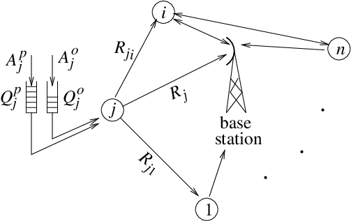
We consider the cellular network illustrated in Fig. 1. The network consists of nodes, each of which has both open and private information to be transmitted to a single base station over the associated uplink channel. When a node is transmitting, every other node overhears the transmission over the associated cross channel. We assume every channel to be iid block fading, with a block size of channel uses. The entire session lasts for blocks, which corresponds to a total of channel uses. We denote the instantaneous achievable rate for the uplink channel of node by , which is the maximum mutual information between output symbols of node and received symbols at the base station over block . Likewise, we denote the rate of the cross channel between nodes and with , which is the maximum mutual information between output symbols of node and input symbols of node over block . Note that there is no actual data transmission between any pair of nodes, but parameter will be necessary, when we evaluate the private rates between node and the base station.
Even though our results are general for all channel state distributions, in numerical evaluations, we assume all channels to be Gaussian and the transmit power to be constant, identical to for all blocks . We represent the uplink channel for node and the cross channel between nodes and with a power gain (magnitude square of the channel gains) and respectively over block . We normalize the power gains such that the (additive Gaussian) noise has unit variance. Then, as ,
| (1) | ||||
| (2) |
Each node has a private and an open message, and respectively, to be transmitted to the base station over channel uses, where and denote the (long-term) private and open information rates respectively, for node . Let the vector of symbols received by node be . To achieve perfect privacy, following constraint must be satisfied by node : for all ,
| (3) |
for any given . We define the instantaneous private information rate of node transmitted privately from node over block as:
| (4) |
where . It was shown in [39] that rate (4) is achievable as and [1] took it a step further and showed that, as , a long-term private information rate of is achievable.
The amount of open traffic, , and private traffic, , injected in the queues at node (shown in Fig. 1) in block are both selected by node at the beginning of each block. Open and private information are stored in separate queues with sizes and respectively. At any given block, a scheduler chooses which node will transmit and the amount of open and private information to be encoded over the block. We use the indicator variable to represent the scheduler decision:
| (5) |
When we evaluate the region of achievable open and private data rate pairs for the single node scenario, in Section III-A, we assume that the transmitting node has perfect causal knowledge of its uplink channel and the cross-channel at every block . Thus, the achievable region of private and open rates constitutes upper bound on the achievable rates for each node, which we find subsequently for the multiuser setting with partial CSI. For private opportunistic scheduler in the multiuser setting, we assume that, each node has perfect causal knowledge of the uplink channel rate, , and its prior distribution. However, we assume that it only has the long-term averages, of its cross-channel rates. To achieve privacy with this level of CSI, private opportunistic scheduler uses an encoding scheme that encodes private information over many packets. When we formulate our problem as that of network utility maximization problem, we only assume knowledge of instantaneous channel gains without requiring the knowledge of prior distribution of channel gains. Hence, private encoding is performed over a single block length unlike the case with private opportunistic scheduler. Additionally, we analyze a more realistic scenario when the instantaneous channel rates are not known perfectly, but estimated with some random additive error. The scheduled transmitter, , will encode at a rate
where is the rate margin, chosen such that the estimation error is taken into account. Note that when , then perfect privacy constraint (3) is violated over block . In such a case, we say that privacy outage has occurred. The probability of privacy outage over block when user is scheduled, is represented as . Since perfect privacy cannot be ensured over every block, we require that expected probability of privacy outage of each user is below a given threshold .
III Achievable Rates and Private Opportunistic Scheduling
In this section, we evaluate the region of private and open rates achievable by a scheduler for multiuser uplink and downlink setting. We start with a single node transmitting, and thus, the scheduler only chooses whether to encode private information at any given point in time or not. We consider the possibility of both the separate and the joint encoding of private and open data. For multiuser transmission, we introduce our scheme, private opportunistic scheduling, evaluate achievable rates and show that it maximizes the sum private information rate achievable by any scheduler. Along with private opportunistic scheduling, we provide the associated physical-layer private encoding scheme that encodes information over many blocks.

III-A Single User Achievable Rates
Consider the single user scenario in which the primary user (node 1) is transmitting information over the primary channel and a single secondary user (node 2) is overhearing the transmission over the secondary channel as shown in Fig. 2. In this scenario, we assume node 2 is passively listening without transmitting information and node 1 has perfect knowledge of instantaneous rates and for all as well as their sample distributions. Over each block , the primary user chooses the rate of private and open information to be transmitted to the intended receiver. As discussed in [40] it is possible to encode open information at a rate over each block , jointly with the private information at rate . For that, one can simply replace the randomization message of the binning strategy of the achievability scheme with the open message, which is allowed to be decoded by the secondary user. In the rest of the section, we analyze both the case in which open information can and cannot be encoded along with the private information. We find the region of achievable private and open information rates, , over the primary channel.
III-A1 Separate encoding of private and open messages
First we assume that each block contains either private or open information, but joint encoding over the same block is not allowed. Recall that is the indicator variable, which takes on a value , if information is encoded privately over block and otherwise. Then, one can find , associated with the point by solving the following integer program:
| (6) | ||||
| subject to | (7) |
where the expectations are over the joint distribution of the instantaneous rates and . Note that, since the channel rates are iid, the solution, will be a stationary policy. Also, a necessary condition for the existence of a feasible solution is . Dropping the block index for simplicity, the problem leads to the following Lagrangian relaxation:
| (8) |
where is the joint pdf of and . For any given values of the Lagrange multiplier and pair, the optimal policy will choose if the integrant is maximized for , or it will choose otherwise. If both and lead to an identical value, the policy will choose one of them randomly. The solution can be summarized as follows:
| (9) |
where is the value of for which , since .
For Gaussian uplink and cross channels described in Section II, the solution can be obtained by plugging (1,2,4) in (9):
| (10) |
The associated solution is graphically illustrated on the space in Fig. 3 for . As the value of varies between 0 and 1, the optimal decision region for increases from the upper half of the first quadrant represented by to the entire first quadrant, i.e., all .


In Fig. 4, the achievable pair of private and open information rates, , is illustrated for iid Rayleigh fading Gaussian channels, i.e., the power gains and have an exponential distribution. We considered two different scenarios in which the mean power gains, , are and , and . The associated boundaries of the rate regions with separate encoding are illustrated with solid curves. To plot these boundaries, we varied from 0 to 1 and calculated the achievable rate pair for each point. Note that the flat portion on the top part of the rate regions for separate encoding corresponds to the case in which Constraint (7) is inactive. It is also interesting to note that as demonstrated in Fig. 4, one can achieve non-zero private information rates even when the mean cross channel gain between node 1 and node 2 is higher than the mean uplink channel gain of node 1.
III-A2 Joint encoding of private and open messages
With the possibility of joint encoding of the open and private information over the same block, the indicator variable implies that the private and open information rates are and respectively over block simultaneously. Otherwise, i.e., if , open encoding is used solely over the block. To find achievable , associated with the point , one needs to consider a slightly different optimization problem this time:
| (11) | ||||
| subject to | (12) |
This optimization problem can be solved in a similar way by employing Lagrangian relaxation as the problem considered in Section III-A1. First, we specify two regions of parameters for which the solution is trivial: 1) if , no solution exists for (11,12), since the uplink channel capacity is not sufficient to meet the desired open rate, ; 2) if , then for all blocks, i.e., all open information will be encoded jointly with private information, since the remaining capacity over that is necessary to support private information is sufficient to serve open information at rate . In this case, Constraint (12) is inactive and the achieved private information rate is .
In all other cases, i.e., , it can be shown that the optimal solution can be achieved by the following probabilistic scheme11 1 Note that the solution of Problem (11,12) is not unique and the described probabilistic solution is just one of them.: For any given block,
| (13) |
independently of and , where . The details of the derivation of the described optimal scheme is given in [41]. With this solution, only a fraction of the blocks contain jointly encoded private and open information, and the remaining fraction of the blocks contain solely open information. Thus, for a given , the achieved private and open information rates can be found as and respectively. Rather surprisingly, it does not matter which blocks contain only open information and which ones contain jointly encoded private and open information, as long as the desired open information rate is met. Consequently, a random scheme that chooses fraction of blocks for open information only and the rest for jointly encoded open and private information suffices to achieve the optimal solution.
By the above analysis, one can conclude that the achievable rate region with joint encoding can be summarized by the intersection of two regions specified by: (i) and (ii) . Any point on the boundary of the region can be achieved by the simple probabilistic scheme described above. One can realize that this region is the maximum achievable rate region, since in our system, the total information rate (private and open) is upper bounded by the capacity, , of uplink channel 1 and the achievable private rate is upper bounded by the secrecy capacity, , of the associated wiretap channel. Thus, there exists no other scheme that can achieve a larger rate region than the one achieved by the simple probabilistic scheme.
In Fig. 4, the achievable pairs of private and open information rates, with joint encoding are illustrated for the iid Rayleigh fading Gaussian channels with the same parameters as the separate encoding scenario. The boundaries of the regions are specified with dashed curves, which are plotted by varying the value of from 0 to 1 and evaluating pair for each value. Similar to the separate encoding scenario, the flat portion on the top part of the regions corresponds to the case in which Constraint (12) is inactive.

III-B Private Opportunistic Scheduling and Multiuser Achievable Rates
In this section, we consider the multiuser setting described in Fig. 1. We introduce private opportunistic scheduling (POS) for the uplink scenario and prove that it achieves the maximum achievable sum private information rate over the set of all schedulers. POS schedules the node that has the largest instantaneous private information rate, with respect to the “best eavesdropper” node, which has the largest mean cross-channel rate. Each node ensures perfect privacy from its best eavesdropper node by using a binning strategy, which requires only the average cross-channel rates to encode the messages over many blocks.
We consider the multiuser uplink scenario given in Fig. 5. We assume every node has perfect causal knowledge of its uplink channel rate, for all blocks and the average cross-channel rates, , for all .
III-B1 Private Opportunistic Scheduling for uplink
We define the best eavesdropper of node as and denote its average cross-channel rate with . Note that does not change from one block to another. In POS, only one of the nodes is scheduled for data transmission in any given block. In particular, in block , we opportunistically schedule node
if and no node is scheduled for private information transmission otherwise, i.e., . In case of multiple nodes achieving the same maximum privacy rate, the tie can be broken at random. Indicator variable takes on a value , if node is scheduled over block and otherwise. We denote the probability that node be scheduled with and the associated uplink channel rate when node is scheduled with , where the expectations are over the conditional joint distribution of the instantaneous rates of all uplink channels, given .
As will be shown shortly, private opportunistic scheduling achieves a private information rate for all . To achieve this set of rates, we use the following private encoding strategy based on binning: To begin, node generates random binary sequences. Then, it assigns each random binary sequence to one of bins, so that each bin contains exactly binary sequences. We call the sequences associated with a bin, the randomization sequences of that bin. Each bin of node is one-to-one matched with a private message randomly. This selection (along with the binary sequences contained in each bin) is revealed to the base station and all nodes before the communication starts. Then, whenever the message to be transmitted is selected by node , the stochastic encoder of that node chooses one of the randomization sequences associated with each bin at random22 2 In case of joint encoding of private and open information, the randomization sequence is chosen appropriately, corresponding to the desired open message., independently and uniformly over all randomization sequences associated with that bin. This particular randomization message is used for the transmission of the message and is not revealed to any of the nodes nor to the base station.
Private opportunistic scheduler schedules node in each block and the transmitter transmits bits of the binary sequence associated with the message of node for all . Thus, asymptotically, the rate of data transmitted by node over blocks is identical to:
| (14) |
for any given from strong law of large numbers. Hence, all of bits, generated by each node is transmitted with probability 1.
III-B2 Achievable uplink rates with private opportunistic scheduling
Theorem 1
With private opportunistic scheduling, a private information rate of is achievable for each node .
The proof of this theorem is based on an equivocation analysis and it can be found in Appendix A. Next we show that private opportunistic scheduling maximizes the achievable sum private information rate among all schedulers.
Theorem 2
Among the elements of the set of all schedulers, , private opportunistic scheduler maximizes the sum privacy uplink rate, . Furthermore, the maximum achievable sum privacy uplink rate is
The proof of Theorem 2 can be found in Appendix B. There, we also show that the individual private information rates given in Theorem 1 are the maximum achievable individual rates with private opportunistic scheduling. Hence the converse of Theorem 1 also holds. Combining Theorems 1 and 2, one can realize that private opportunistic scheduling achieves the maximum achievable sum private information rate. Thus, one cannot increase the individual private information rate a single node achieves with POS by an amount , without reducing another node’s private information rate by more than .
Next, we find the boundary of the region of achievable sum open and sum private uplink rate pair with joint encoding of private and open information. In opportunistic scheduling [38, 29] without any privacy constraint, the user with the best uplink channel is scheduled for all blocks . Hence, the associated achievable rate can be written as . Since this constitutes an upper bound for the achievable cumulative information rate [38], the total private and open information rate in our system cannot exceed . Combining this with Theorem 2, we can characterize an outer bound for the achievable rate region for the sum rates as follows: (i) ; (ii) . Next we illustrate this region and discuss how the entire region can be achieved by POS along with joint encoding of private and open messages.

The boundaries of this region is illustrated in Fig. 6 for a 5-node and a 10-node system. We assume all channels to be iid Rayleigh fading with mean uplink channel power gain and mean cross channel power gain or in two separate scenarios for all . Noise is additive Gaussian with unit variance and transmit power . In these graphs, sum rates are normalized with respect to the number of nodes. One can observe that, the achievable sum rate per node decreases from to bits/channel use/node for and from to bits/channel use/node for as the number of nodes increases from to . Also, the open rate per node drops from to bits/channel use/node with the same increase in the number of nodes.
Note that, any point on the part of the boundary specified by (i) above (flat portion on the top part) is achievable by POS and jointly encoding the private information with the appropriate amount of open information used as a randomization message. For instance, the corner point of two boundaries (intersection of (i) and (ii)) is achieved when open information is used completely in place of randomization messages by all nodes. All points on the part of the boundary specified by (ii) can be achieved by time-sharing between the corner point, and point , which corresponds to opportunistic scheduling (without privacy).
IV Dynamic Control of Private Communications
In Section III, we determined the achievable private information rate regions associated with private opportunistic scheduling which encodes messages over many blocks. Hence, the delay of decoding private information may be extremely long. Also, the private opportunistic scheduler was based on the availability of full CSI on the uplinks, and long-term average of cross-channel rates. In this section, we investigate a dynamic control algorithm which does not rely on any a priori knowledge of distributions of direct- or cross-channel rates, and the private information is encoded over a single block. Hence, a private message can be decoded with a maximum delay of only a single block duration. Note that even though by encoding over many blocks one may achieve higher private information rates, decoding delay may be a more important concern in many practical scenarios.
In particular, each message and are broken into a sequence of messages, and respectively and each element of the sequence is encoded into an individual packet, encoded over block . The delay-limited dynamic cross-layer control algorithm opportunistically schedules the nodes with the objective of maximizing the total expected utility gained from each packet transmission while maintaining the stability of private and open traffic queues. The algorithm takes as input the queue lengths and instantaneous direct- and cross-channel rates, and gives as output the scheduled node and its privacy encoding rate. In the sequel, we only consider joint encoding of private and open information as described in Section III-A2.
Let and be the utilities obtained by node from private and open transmissions over block respectively. Let us define the instantaneous private information rate of node as , where was defined in (4). Also, the instantaneous open rate, , is the amount of open information node transmits over block . The utility over block depends on rates , and . In general, this dependence can be described as and . Assume that , , and , are concave non-decreasing functions. We also assume that the utility of a private transmission is higher than the utility of open transmission at the same rate. The amount of open traffic , and private traffic injected in the queues at node have long term arrival rates and respectively. Our objective is to support a fraction of the traffic demand to achieve a long term private and open throughput that maximizes the sum of utilities of the nodes.
IV-A Perfect Knowledge of Instantaneous CSI
We first consider the case when every node has perfect causal knowledge of its uplink channel rate, , and cross-channel rates to all other nodes in the network , , for all blocks . The dynamic control algorithm developed for this case will then provide a basis for the algorithm that we are going to develop for a more realistic case when cross-channel rates are not known perfectly. We aim to find the solution of the following optimization problem:
| (15) | ||||
| (16) |
The objective function in (15) calculates the total expected utility of open and private communications where expectation is taken over the random achievable rates (random channel conditions), and possibly over the randomized policy. The constraint (16) ensures that private and open injection rates are within the achievable rate region supported by the network denoted by . In the aforementioned optimization problem, it is implicitly required that perfect secrecy condition given in (3) is satisfied in each block as .
The proposed cross-layer dynamic control algorithm is based on the stochastic network optimization framework developed in [37]. This framework allows the solution of a long-term stochastic optimization problem without requiring explicit characterization of the achievable rate region, .
We assume that there is an infinite backlog of data at the transport layer of each node. Our proposed dynamic flow control algorithm determines the amount of open and private traffic injected into the queues at the network layer. The dynamics of private and open traffic queues is given as follows:
| (17) | ||||
| (18) |
where , and the service rates of private and open queues are given as,
where and are indicator functions taking value when transmitting jointly encoded private and open traffic, or when transmitting only open traffic over block respectively. Also note that at any block , .
Control Algorithm: The algorithm is a simple index policy and it executes the following steps in each block :
(1) Flow control: For some , each node injects private and open bits, where
(2) Scheduling: Schedule node and transmit jointly encoded private and open traffic (), or only open () traffic, where
and for each node , encode private data over each block at rate
and transmit open data at rate
Optimality of Control Algorithm
The optimality of the algorithm can be shown using the Lyapunov optimization theorem [37]. Before restating this theorem, we define the following parameters. Let be the queue backlog process, and let our objective be the maximization of time average of a scalar valued function of another process while keeping finite. Also define as the drift of some appropriate Lyapunov function .
Theorem 3
(Lyapunov Optimization) [37] For the scalar valued function , if there exists positive constants , , , such that for all blocks and all unfinished work vector the Lyapunov drift satisfies:
| (19) |
then the time average utility and queue backlog satisfy:
| (20) | ||||
| (21) |
where is the maximal value of and .
For our purposes, we consider private and open unfinished work vectors as , and . Let be quadratic Lyapunov function of private and open queue backlogs defined as:
| (22) |
Also consider the one-step expected Lyapunov drift, for the Lyapunov function (22) as:
| (23) |
The following lemma provides an upper bound on .
Lemma 1
| (24) |
where is a constant.
The proof of Lemma 1 is given in Appendix C. Now, we present our main result showing that our proposed dynamic control algorithm can achieve a performance arbitrarily close to the optimal solution while keeping the queue backlogs bounded.
Theorem 4
IV-B Imperfect Knowledge of Instantaneous CSI
In the previous section, we performed our analysis assuming that at every block exact instantaneous cross-channel rates are available. However, unlike the uplink direct channel rate which can be determined by the base station prior to the data transmission (e.g., via pilot signal transmission), cross-channel rates are harder to be estimated. Indeed, in a non-cooperative network in which nodes do not exchange their CSI, the cross-channel rates can only be inferred by node from the received signals over the reverse channel as nodes are transmitting to the base station. Hence, at a given block, nodes only have a posteriori channel distribution. Based on this a posteriori channel distribution, nodes may estimate CSI of their cross-channels.
Let us denote the estimated rate of the cross-channel with . We also define cross-channel rate margin as the cross-channel rate a node uses when it encodes private information. More specifically, node encodes its private information at rate:
| (25) |
i.e., is the rate of the randomization message node uses in the random binning scheme for privacy. Note that, if , then node will not meet the perfect secrecy constraint at block , leading to a privacy outage. In the event of a privacy outage, the privately encoded message is considered as an open message. The probability of privacy outage over block for the scheduled node , given the estimates of the cross channel rates is:
| (26) |
Compare the aforementioned definition of privacy outage with the channel outage [42] experienced in fast varying wireless channels. In time-varying wireless channels, channel outage occurs when received signal and interference/noise ratio drops below a threshold necessary for correct decoding of the transmitted signal. Hence, the largest rate of reliable communications at a given outage probability is an important measure of channel quality. In the following, we aim to determine utility maximizing achievable privacy and open transmission rates for given privacy outage probabilities. In particular, we consider the solution of the following optimization problem:
| (27) | ||||
| (28) | ||||
| (29) |
where is the tolerable privacy outage probability. Aforementioned optimization problem is the same as the one given for perfect CSI except for the last constraint. The additional constraint (29) requires that only a certain prescribed proportion of private transmissions are allowed to violate the perfect privacy constraint. Due to privacy outages we define private goodput of user as . Note that private goodput only includes private messages for which perfect privacy constraint is satisfied. All private messages for which (3) is violated are counted as successful open transmissions.
Similar to the perfect CSI case, we argue that a dynamic policy can be used to achieve asymptotically optimal solution. Unlike the algorithm given in the perfect CSI case, the algorithm for imperfect CSI first determines the private data encoding rate so that the privacy outage constraint (29) is satisfied in current block. Hence, the private encoding rate at a particular block is determined by the estimated channel rates and the privacy outage constraint.
Control Algorithm: Similar to the perfect CSI case, our algorithm involves two steps in each block :
(1) Flow Control: For some , each node injects private and open bits, where
| (30) |
(2) Scheduling: Schedule node and transmit jointly encoded private and open traffic () or only open () traffic, where
For each node , encode private data over each block at rate
and transmit open data at rate
Optimality of Control Algorithm
The optimality of the control algorithm with imperfect CSI can be shown in a similar fashion as for the control algorithm with perfect CSI. We use the same Lyapunov function defined in (22) which results in the same one-step Lyapunov drift function (23). Hence, Lemma 1 also holds for the case of imperfect CSI, but with a different constant due to the fact that higher maximum private information rates can be achieved by allowing privacy outages.
Lyapunov Optimization Theorem suggests that a good control strategy is the one that minimizes the following:
| (31) |
In (31), expectation is over all possible channel states. The expected utility for private and open transmissions are respectively given as:
| (32) | ||||
| (33) |
Note that (32)-(33) are obtained due to Constraint (29). By combining Lemma 1 with (32)-(33) we may obtain an upper bound for (31), as follows:
| (34) |
Now, it is clear that the proposed dynamic control algorithm minimizes the right hand side of (34). The steps of proving the optimality of the dynamic control algorithm are exactly the same as those given in Theorem 4, and hence, we skip the details.
V Numerical Results
In our numerical experiments, we considered a network consisting of ten nodes and a single base station. The direct channel between a node and the base station, and the cross-channels between pairs of nodes are modeled as iid Rayleigh fading Gaussian channels. Thus, direct-channel and cross-channel power gains are exponentially distributed with means chosen uniformly randomly in the intervals , and , respectively. The noise normalized power is . In our simulations, we consider both of the cases when perfect instantaneous CSI is available, and when instantaneous CSI can only be estimated with some error. Unless otherwise indicated, in the case of imperfect CSI, we take the tolerable privacy outage probability as . We assumed the use of an unbiased estimator for the cross-channel power gains and modeled the associated estimation error with a Gaussian random variable:
where for all . Gaussian estimation error can be justified as discussed in [43] or by the use of a recursive ML estimator as in [44]. Unless otherwise stated, we take , i.e., the estimation error is rather significant relative to the mean cross-channel gain. Note that, in this section, we choose the margin such that
We consider logarithmic private and open utility functions where the private utility is times more than open utility at the same rate. More specifically, we take for a scheduled node , , and . We take in all the experiments except for the one inspecting the effect of . The rates depicted in the graphs are per node arrival or service rates calculated as the total arrival or service rates achieved by the network divided by the number of nodes, i.e., the unit of the plotted rates is bits/channel use/node. Finally, for perfect CSI, we only plot the service rates since arrival and service rates are identical.
In Fig. 7a-7b, we investigate the effect of system parameter in our dynamic control algorithm. Fig. 7a shows that for , long-term utilities converge to their optimal values fairly closely. It is also observed that CSI estimation error results in a reduction of approximately 25% in aggregate utility. Fig. 7b depicts the well-known relationship between and queue backlogs, where queue backlogs increase when is increased.


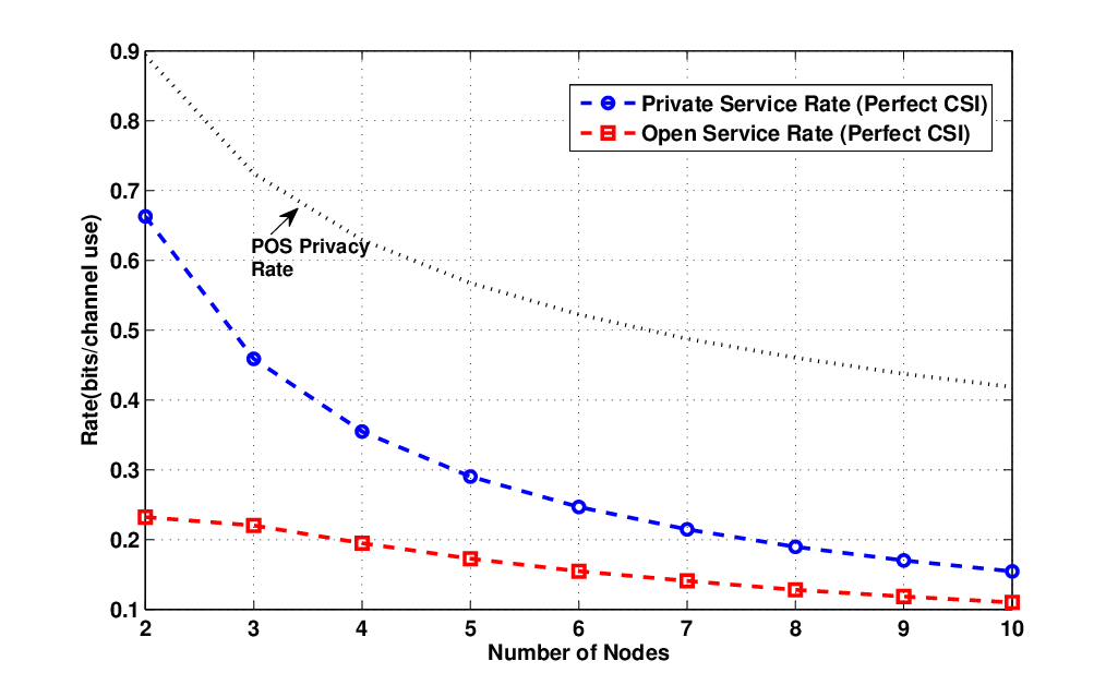
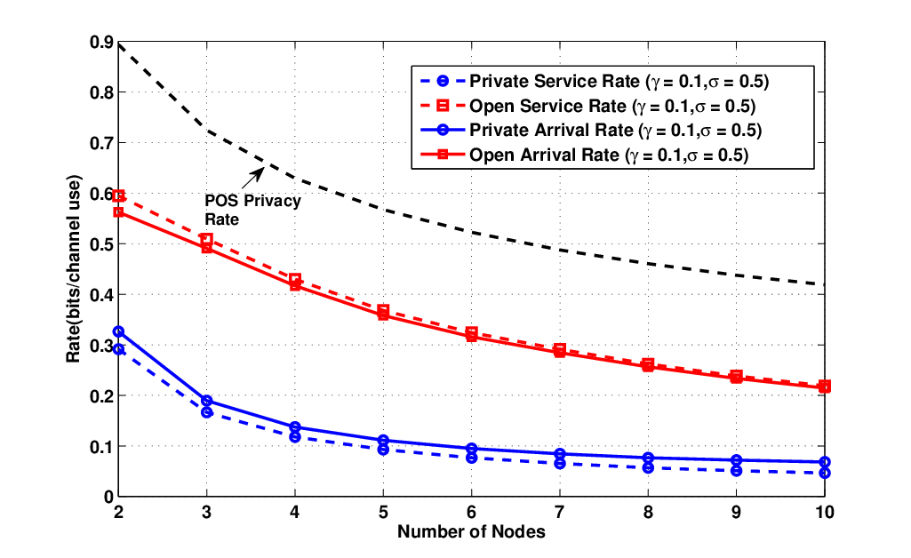
In Fig. 8a-8b, the effect of increasing number of nodes on the achievable private and open rates obtained with the proposed dynamic control algorithm is shown. In both figures, the private information rate achieved by POS algorithm given in Section III is also depicted. From Fig. 8a, we first notice that by using the dynamic control algorithm which is based only on the instantaneous CSI, the private service rate is reduced by more than 25% as compared to the maximum private information rate achieved by POS which uses a priori CSI to encode over many blocks. This difference increases with increasing number of nodes. However, for both POS and dynamic control algorithms, the achievable rates decrease with increasing number of nodes since more nodes overhear ongoing transmissions. Meanwhile, open service rate also decreases due to the fact that there is a smaller number of transmission opportunities per node with increasing number of nodes. Fig. 8b depicts that private service rate has decreased by approximately 50% due to CSI estimation errors. It is also interesting to note that private arrival rate is higher than the private service rate, since all private messages for which perfect privacy constraint cannot be satisfied are considered as successful open messages. Hence, open service rate is observed to be higher than the open arrival rate.
We next analyze the effect of , which can also be interpreted as the ratio of utility of private and open transmissions taking place at the same rate. We call this ratio private utility gain. Fig. 9a shows that when private utility gain is greater than 5, then the private and open service rates converge to their respective limits. These limits depend on the channel characteristics, and their sum is approximately equal to the maximum achievable rate of the channel. However, when there is CSI estimation error, Fig. 9b shows that although an identical qualitative relationship between arrival rates and private utility gain is still observed, private service rate is lower than the private arrival rate by a fraction of almost uniformly in the range of .


In Fig. 10a, we investigate the effect of the tolerable privacy outage probability. It is interesting to note that private service rate increases initially with increasing tolerable outage probability. This is because for low values, in order to satisfy the tight privacy outage constraint, a low instantaneous private information rate is chosen. However, when is high more privacy outages are experienced at the expense of higher instantaneous private information rates. This is also the reason why we observe that the difference between the private service and arrival rates is increasing. We note that when CSI estimation error is present, the highest private service rate is obtained when is approximately equal to . The highest private service rate with CSI estimation error is approximately 30% lower than the private service rate with the perfect CSI.
We finally investigate the effect of the quality of CSI estimator in Fig. 10b. For this purpose, we vary the standard deviation of the Gaussian random variable modeling the estimation error. As expected the highest private service rate is obtained when . However, it is important to note that this value is still lower than the private service rate with perfect CSI, since privacy outages are still permitted in % of private transmissions. We have also investigated the performance of the dynamic control algorithm when a posteriori CSI distribution is not available. In this case, scheduling and flow control decisions are based only on the mean cross channel gains. When only mean cross channel gains are available, the achieved private service rate per node is approximately equal to bits per channel use, which is significantly lower than the private service rate with perfect CSI. In particular, it is only when the standard deviation of the estimation error is that the private service rate with noisy channel estimator has the same private service rate achievable utilizing only mean channel gains.


VI Conclusions
In this paper, we studied the achievable private and open information rate regions of single- and multi-user wireless networks with node scheduling. We introduce private opportunistic scheduling along with a private encoding strategy, and show that it maximizes the sum private information rate for both multiuser uplink communication when perfect CSI is available for only the main uplink channels. Then, we described a cross-layer dynamic algorithm that works without prior distribution of channel states. We prove that our algorithm, which is based on simple index policies, achieves utility arbitrarily close to achievable optimal utility. The simulation results also verify the efficacy of the algorithm.
As a future direction, we will investigate the cooperation among nodes, e.g., intelligent jamming from cooperating nodes, as a means to improve the achievable private information rates. We will also investigate an extension of the dynamic control policy for imperfect CSI, where the optimal privacy outage probability is also determined by the algorithm.
References
- [1] P. K. Gopala, L. Lai, and H. El Gamal, “On the secrecy capacity of fading channels,” IEEE Trans. Inform. Theory, vol. 54, pp. 4687–4698, Oct. 2008.
- [2] J. Barros and M. R. D. Rodrigues, “Secrecy capacity of wireless channels,” in Proc. IEEE Int. Symposium Inform. Theory, (Seattle, WA), pp. 356–360, July 2006.
- [3] Y. Liang, H. V. Poor, and S. Shamai (Shitz), “Secure communication over fading channels,” IEEE Trans. Inform. Theory, vol. 54, pp. 2470–2492, June 2008.
- [4] L. Lai, H. El Gamal, and H. V. Poor, “The wiretap channel with feedback: Encryption over the channel,” IEEE Trans. Inform. Theory, vol. 54, pp. 5059 – 5067, Nov. 2008.
- [5] E. Ardestanizadeh, M. Franceschetti, T. Javidi, and Y. Kim, “The secrecy capacity of the wiretap channel with rate-limited feedback,” IEEE Trans. Inform. Theory, 2009. To appear.
- [6] D. Gunduz, R. Brown, and H. V. Poor, “Secret communication with feedback,” in Proc. IEEE Intl. Symposium on Information Theory and its Applications, (Auckland, New Zealand), Dec. 2008.
- [7] A. Khisti and G. W. Wornell, “Secure transmission with multiple antennas: The MISOME wiretap channel,” IEEE Trans. Inform. Theory, 2009. To appear.
- [8] F. Oggier and B. Hassibi, “The secrecy capacity of the MIMO wiretap channel,” IEEE Trans. Inform. Theory, Oct. 2007. Submitted.
- [9] S. Shafiee, N. Liu, and S. Ulukus, “Towards the secrecy capacity of the Gaussian MIMO wire-tap channel: The 2-2-1 channel,” IEEE Trans. Inform. Theory, vol. 55, pp. 4033 – 4039, Sept. 2009.
- [10] R. Liu and H. V. Poor, “Secrecy capacity region of a multi-antenna Gaussian broadcast channel with confidential messages,” IEEE Trans. Inform. Theory, vol. 55, pp. 1235–1249, Mar. 2009.
- [11] L. Lai and H. El Gamal, “The relay-eavesdropper channel: Cooperation for secrecy,” IEEE Trans. Inform. Theory, vol. 54, pp. 4005–4019, Sept. 2008.
- [12] E. Tekin and A. Yener, “The Gaussian multiple access wire-tap channel,” IEEE Trans. Inform. Theory, vol. 54, pp. 5747 – 5755, Dec. 2008.
- [13] Y. Liang and H. V. Poor, “Multiple access channels with confidential messages,” IEEE Trans. Inform. Theory, vol. 54, pp. 976–1002, Mar. 2008.
- [14] A. Khisti, A. Tchamkerten, and G. W. Wornell, “Secure broadcasting over fading channels,” IEEE Trans. Inform. Theory, vol. 54, pp. 2453–2469, June 2008.
- [15] M. Bloch, J. Barros, M. R. D. Rodrigues, and S. W. McLaughlin, “Wireless information-theoretic security,” IEEE Trans. Inform. Theory, vol. 54, pp. 2515–2534, June 2008.
- [16] Z. Li, R. Yates, and W. Trappe, “Secure communication over wireless channels,” in Proc. Inform. Theory and Appl. Workshop, (La Jolla, CA.), Jan. 2007.
- [17] O. Simeone and A. Yener, “The cognitive multiple access wire-tap channel,” in Proc. Conf. Inform. Science and Systems, (Baltimore, MD), Mar. 2009.
- [18] P. Parada and R. Blahut, “Secrecy capacity of SIMO and slow fading channels,” in Proc. IEEE Int. Symposium Inform. Theory, (Adelaide, Australia), pp. 2152–2155, Sep. 2005.
- [19] R. Liu, I. Maric, R. D. Yates, and P. Spasojevic, “The discrete memoryless multiple access channel with confidential messages,” in Proc. IEEE Int. Symposium Inform. Theory, (Seattle, WA), pp. 957–961, July 2006.
- [20] Y. Oohama, “Relay channels with confidential messages,” IEEE Trans. Inform. Theory, Nov. 2006. Submitted.
- [21] E. Ekrem and S. Ulukus, “The secrecy capacity region of the Gaussian MIMO multi-receiver wiretap channel,” IEEE Trans. Inform. Theory, Mar. 2009. Submitted.
- [22] M. Yuksel, X. Liu, and E. Erkip, “A secure communication game with a relay helping the eavesdropper,” in Proc. IEEE Information Theory Workshop, (Taormina, Italy), Oct. 2009. To appear.
- [23] S. Ali, A. Fakoorian, and A. L. Swindlehurst, “Mimo interference channel with confidential messages: Achievable secrecy rates and precoder design,” IEEE Trans. Inf. Forensics and Security, vol. 6, pp. 640–649, Sep. 2011.
- [24] J. Li, A. P. Petropulu, and S. Weber, “On cooperative relaying schemes for wireless physical layer security,” IEEE Trans. Signal Processing, vol. 59, pp. 4985–4997, Oct. 2011.
- [25] J. Chen, R. Zhang, L. Song, Z. Han, and B. Jiao, “Joint relay and jammer selection for secure two-way relay networks,” IEEE Trans. Inf. Forensics and Security, vol. 7, pp. 310–320, Feb. 2012.
- [26] R. Liu, Y. Liang, H. V. Poor, and P. Spasojevic, “Secure nested codes for type II wiretap channels,” in Proc. IEEE Information Theory Workshop, (Lake Tahoe, CA), Sep. 2-6 2007.
- [27] M. Bloch, A. Thangaraj, S. W. McLaughlin, and J.-M. Merolla, “LDPC based secret key agreement over the gaussian wiretap channel,” in Proc. IEEE Int. Symposium Inform. Theory, (Seattle, WA), pp. 1179 – 1183, July 2006.
- [28] L. Tassiulas and A. Ephremides, “Jointly optimal routing and scheduling in packet ratio networks,” IEEE Transactions on Information Theory, vol. 38, pp. 165 –168, Jan. 1992.
- [29] X. Liu, E. K. P. Chong, and N. B. Shroff, “A framework for opportunistic scheduling in wireless networks,” Computer Networks, vol. 41, no. 4, pp. 451–474, 2003.
- [30] J. Huang, V. Subramanian, R. Agrawal, and R. Berry, “Downlink scheduling and resource allocation for ofdm systems,” IEEE Transactions on Wireless Communications, vol. 8, no. 1, pp. 288 –296, 2009.
- [31] R. Urgaonkar and M. J. Neely, “Opportunistic scheduling with reliability guarantees in cognitive radio networks,” IEEE Trans. Mob. Comput., vol. 8, no. 6, pp. 766–777, 2009.
- [32] J. J. Jaramillo and R. Srikant, “Optimal scheduling for fair resource allocation in ad hoc networks with elastic and inelastic traffic,” in INFOCOM, pp. 2231–2239, 2010.
- [33] A. Stolyar, “Greedy primal-dual algorithm for dynamic resource allocation in complex networks,” Queueing Systems, vol. 54, pp. 203–220, 2006. 10.1007/s11134-006-0067-2.
- [34] F. P. Kelly, A. K. Maulloo, and D. K. H. Tan, “Rate Control for Communication Networks: Shadow Prices, Proportional Fairness and Stability,” The Journal of the Operational Research Society, vol. 49, no. 3, pp. 237–252, 1998.
- [35] S. H. Low and D. E. Lapsley, “Optimization flow control-i: basic algorithm and convergence,” IEEE/ACM Trans. Netw., vol. 7, no. 6, pp. 861–874, 1999.
- [36] X. Wang and K. Kar, “Cross-layer rate control for end-to-end proportional fairness in wireless networks with random access,” in MobiHoc, pp. 157–168, 2005.
- [37] L. Georgiadis, M. J. Neely, and L. Tassiulas, “Resource allocation and cross-layer control in wireless networks,” Foundations and Trends in Networking, vol. 1, no. 1, 2006.
- [38] R. Knopp and P. A. Humblet, “Information capacity and power control in single-cell multiusercommunications,” in Proc. IEEE Int. Conf. Commun., vol. 1, (Seattle, WA), pp. 331–335, Jun. 18-22, 1995.
- [39] A. D. Wyner, “The wire-tap channel,” The Bell System Technical Journal, vol. 54, pp. 1355–1387, Oct. 1975.
- [40] I. Csiszr and J. Krner, “Broadcast channels with confidential messages,” IEEE Trans. Inform. Theory, vol. 24, pp. 339–348, May 1978.
- [41] C. E. Koksal and O. Ercetin, “Control of wireless networks with secrecy,” technical report, 2010. http://arxiv.org/abs/cs/1101.3444.
- [42] D. Tse and P. Viswanath, Fundamentals of Wireless Communication. New York: Cambridge University Press, 2005.
- [43] P. Frenger, “Turbo decoding for wireless systems with imperfect channel estimates,” IEEE Transactions on Communications, vol. 48, no. 9, pp. 1437 –1440, 2000.
- [44] C. E. Koksal and P. Schniter, “Robust rate-adaptive wireless communication using ack/nak-feedback,” IEEE Trans. on Signal Processing, 2012. to appear.
- [45] M. J. Neely, “Energy optimal control for time-varying wireless networks,” IEEE Transactions on Information Theory, vol. 52, no. 7, pp. 2915–2934, 2006.
Appendix A Proof of Theorem 1
Let us further introduce the following notation:
: randomization sequence associated with message ,
: transmitted vector of () symbols over block ,
: the transmitted signal over block , whenever (i.e., node is the active transmitter)
: the received vector of symbols at node ( for the base station) over block ,
: the received signal at node over block , whenever (i.e., node is the active transmitter). We use for the received signal by the base station.
The equivocation analysis follows directly for the described privacy scheme: For any given node , we have
| (36) | ||||
| (37) | ||||
| (38) | ||||
| (39) | ||||
| (40) | ||||
| (41) | ||||
| (42) | ||||
| (43) | ||||
| (44) |
with probability 1, for any positive triplet and arbitrarily small , as go to . Here, (36) follows since ( forms a Markov chain for all and data processing inequality), (37) is by the chain rule, (38) follows from the application of Fano’s inequality (as we choose the rate of the randomization sequence to be , which allows for the randomization message to be decoded at node , given the bin index), (39) follows from the chain rule and that forms a Markov chain, (40) holds since as the transmitted symbol sequence is determined w.p.1 given , (41) follows from the chain rule, (42) holds since is an entry of vector , (43) holds because the fading processes are iid, and finally (44) follows from strong law of large numbers.
Thus, with the described privacy scheme, the perfect privacy constraint is satisfied for all nodes, since for any , we have
| (45) |
for any given . We just showed that, with private opportunistic scheduling, a private information rate of is achievable for any given node . ∎
Appendix B Proof of Theorem 2
The proof uses the notation introduced in the first paragraph of Appendix A. To meet the perfect secrecy constraint, it is necessary and sufficient to guarantee for all nodes . Since , one can write an equivalent condition on the sum mutual information over each node:
| (46) | ||||
| (47) | ||||
| (48) | ||||
| (49) | ||||
| (50) | ||||
| (51) | ||||
| (52) | ||||
| (53) | ||||
| (54) | ||||
| (55) |
with probability 1, for any positive and triplet as go to . Here, (46) follows from the definition of and that ; (47) follows from the chain rule and Fano’s inequality (as since the message pair can be decoded with arbitrarily low probability of error given ); (48) is from the data processing inequality as forms a Markov chain; (49) and (50) follow from the chain rule; (51) follows from the data processing inequality; (52) follows since node decodes message with arbitrarily low probability of error ; (53) holds since the fading processes are iid; (54) holds because private opportunistic scheduler chooses for all ; and finally (55) follows by an application of the strong law of large numbers. The above derivation leads to the desired result:
| (56) |
We complete the proof noting that the above sum rate is achievable by private opportunistic scheduling as shown in (44). ∎
Note that, from the above steps, we can also see that the individual private information rates given in Theorem 1 are the maximum achievable individual rates with private opportunistic scheduling. This is due to the fact that, for any node , with private opportunistic scheduling, the above derivation lead to:
| (57) |
for any as . Consequently, with private opportunistic scheduling, no node can achieve any individual privacy rate above that given in (57), hence the converse of Theorem 1 also holds.
Appendix C Proof of Lemma 1
Proof: Since the maximum transmission power is finite, in any interference-limited system transmission rates are bounded. Let and be the maximum private and open rates for user , which depends on the channel states. Also assume that the arrival rates are bounded, i.e., and be the maximum number of private and open bits that may arrive in a block for each user. Hence, the following inequalities can be obtained for each private queue:
| (58) |
where . The same line of derivation can be performed for open queues to obtain:
| (59) |
where .
Appendix D Proof of Theorem 4
Proof: Lyapunov Optimization Theorem [37] suggests that a good control strategy is the one that minimizes the following:
| (60) |
By rearranging the terms in (61) it is easy to observe that our proposed dynamic network control algorithm minimizes the right hand side of (61).
If the private and open arrival rates are in the feasible region, it has been shown in [45] that there must exist a stationary scheduling and rate control policy that chooses the users and their transmission rates independent of queue backlogs and only with respect to the channel statistics. In particular, the optimal stationary policy can be found as the solution of a deterministic policy if a priori channel statistics are known.
Let be the optimal value of the objective function of the problem (15)-(16) obtained by the aforementioned stationary policy. Also let and be optimal private and open traffic arrival rates found as the solution of the same problem. In particular, the optimal input rates and could in principle be achieved by the simple backlog-independent admission control algorithm of including all new arrivals for a given node in block independently with probability . Then, the right hand side (RHS) of (61) can be rewritten as
| (62) |
Also, since , i.e., arrival rates are strictly interior of the rate region, there must exist a stationary scheduling and rate allocation policy that is independent of queue backlogs and satisfies the following:
| (63) | ||||
| (64) |
Clearly, any stationary policy should satisfy (61). Recall that our proposed policy minimizes RHS of (61), and hence, any other stationary policy (including the optimal policy) has a higher RHS value than the one attained by our policy. In particular, the stationary policy that satisfies (63)-(64), and implements aforementioned probabilistic admission control can be used to obtain an upper bound for the RHS of our proposed policy. Inserting (63)-(64) into (62), we obtain the following upper bound for our policy:
| (65) |
This is exactly in the form of Lyapunov Optimization Theorem given in Theorem 3, and hence, we can obtain bounds on the performance of the proposed policy and the sizes of queue backlogs as given in Theorem 4. ∎
![[Uncaptioned image]](1101.3444v3/emre.png) |
C. Emre Koksal C. Emre Koksal received the B.S. degree in electrical engineering from the Middle East Technical University, Ankara, Turkey, in 1996, and the S.M. and Ph.D. degrees from the Massachusetts Institute of Technology (MIT), Cambridge, in 1998 and 2002, respectively, in electrical engineering and computer science. He was a Postdoctoral Fellow in the Networks and Mobile Systems Group in the Computer Science and Artificial Intelligence Laboratory, MIT and a Senior Researcher jointly in the Laboratory for Computer Communications and the Laboratory for Information Theory at EPFL, Lausanne, Switzerland. Since 2006, he has been an Assistant Professor in the Electrical and Computer Engineering Department, Ohio State University, Columbus, Ohio. His general areas of interest are wireless communication, communication networks, information theory, stochastic processes, and financial economics. He is the recipient of the National Science Foundation CAREER Award (2011), the OSU College of Engineering Lumley Research Award (2011), and the co-recipient of an HP Labs - Innovation Research Award. The paper he co-authored was a best student paper candidate in MOBICOM 2005. |
![[Uncaptioned image]](1101.3444v3/ozgur.png) |
Ozgur Ercetin received the BS degree in electrical and electronics engineering from the Middle East Technical University, Ankara, Turkey, in 1995 and the MS and PhD degrees in electrical engineering from the University of Maryland, College Park, in 1998 and 2002, respectively. Since 2002, he has been with the Faculty of Engineering and Natural Sciences, Sabanci University, Istanbul. He was also a visiting researcher at HRL Labs, Malibu, CA, Docomo USA Labs, CA, and The Ohio State University, OH. His research interests are in the field of computer and communication networks with emphasis on fundamental mathematical models, architectures and protocols of wireless systems, and stochastic optimization. |
![[Uncaptioned image]](1101.3444v3/yunus.png) |
Yunus Sarikaya received the BS and MS degrees in telecommunications engineering from Sabanci University, Istanbul, Turkey, in 2006 and 2008, respectively. He is currently PhD student in electrical engineering at Sabanci University. His research interests include optimal control of wireless networks, stochastic optimization and information theoretical security. |