Magnetic Excitations in the Site-Centered Stripe Phase:
Spin Wave Theory of Coupled Three-Leg Ladders
Abstract
The success of models of coupled two-leg spin ladders in describing the magnetic excitation spectrum of La2-xBaxCuO4 had been interpreted previously as evidence for bond-centered stripes. In a recent article, however, we have determined the magnetic coupling induced by the charge stripes between bond- or site-centered spin stripes modeled by two- or three-leg ladders, respectively. We found that only the site-centered models order. We further indicated excellent agreement of a fully consistent analysis of coupled three-leg ladders using a spin wave theory of bond with the experimental data. Here, we provide a full and detailed account of this analysis.
pacs
74.72.-h, 74.20.Mn, 75.10.-b, 75.25.-jI Introduction
Twenty years after the discovery, the mechanism of high- superconductivity in the copper oxide materials is still considered one of the most important outstanding problem in contemporary physics [1, 2]. The materials are described by mobile charge carriers (holes) doped into a quasi-twodimensional spin 1/2 antiferromagnet [3, 4]. Inelastic neutron scattering experiments have revealed a magnetic resonance peak [5, 6] and, in some compounds, periodic modulations in the spin and charge density (stripes) [7, 8, 9, 10, 11, 12, 13, 14]. Tranquada et al. [15] found that the magnetic excitation spectrum of stripe ordered La1.875Ba0.125CuO4 looks similar to disordered YBa2Cu3O6+x [6] or Bi2Sr2CaCu2O8+δ [16], and observed that the data are consistent with bond-centered stripes modeled by two-leg ladders. This experiment is considered of key importance for the field, as it it may provide the decisive hint as to within which framework copper oxide superconductors may be understood.
With regard to such a framework, there is no consensus at present, but a fierce competition among different schools of thought. One of these schools [10, 11, 13, 14] attributes the unusual properties of the doped, two-dimensional antiferromagnets to their propensity to form stripes, or their proximity to a quantum critical point (QCP) at which stripe order sets in. The resulting picture is highly appealing. Static stripes have been observed [9, 12] only in certain compounds, most notably La2-xSrxCuO4 at a hole doping concentration , and are known to suppress superconductivity. On the other hand, the mere existence of stripes would impose an effective one-dimensionality, and hence provide a framework to formulate fractionally quantized excitations. This one-dimensionality would be roughly consistent with an enormous body of experimental data on the cuprates, including the electron spectral functions seen in angle-resolved photo emission spectroscopy (ARPES). The charge carriers, the holons, would predominantly reside in the charge stripes, as they could maximize their kinetic energy in these antiferromagnetically disordered regions. In the spin stripes, by contrast, the antiferromagnetic exchange energy between the spins would be maximized, at the price of infringing on the mobility of the charge carriers. Most importantly, the spin stripes would impose a coupling between the charge stripes, which would yield an effective, pairwise confinement between the low-energy spinon and holon excitations residing predominantly in the charge stripes. The mechanism of confinement would be similar to that of coupled spin chains or spin ladders [17, 18, 19]. The holes would be described by spinon-holon bound states, and the dominant contribution to the magnetic response measured in Tranquada’s as well as all other neutron scattering experiments would come from spinon-spinon bound states.


The similarity of the “hour-glass” spectrum shown in Fig. 4b of Tranquada et al. [15] (which is reproduced for comparison in Fig. 1b) with the “elephants trousers” observed by Bourges et al. [6] (which are reproduced for comparison in Fig. 1b) provides the most striking evidence in favor of the picture advocated by this school, which attributes the anomalous properties of generic, disordered CuO superconductors to the formation of dynamic (rather than static) stripes, which fluctuate on time scales which are slow compared to the energy scales of most experimental probes. This picture is considered to receive additional support by Xu et al. [20], who observed that the magnetic response of La1.875Ba0.125CuO4 at higher energies is independent of temperature, while the stripe order melts at about . Measurements on ‘untwinned’ samples of YBa2Cu3O6.6, where one would expect the dynamical stripes to orient themselves along one of the axis, however, exhibit a strong anisotropy in the response only at energies below the resonance [21], while the response is fourfold rotationally symmetric at higher energies [22]. We believe, however, that this only indicates that the formation of stripe correlations, be it static or dynamic, is a low energy phenomenon, while the high energy response probes itinerant antiferromagnets at length scales on which the stripes are essentially invisible.
An extremely appealing feature of the experiment by Tranquada et al. [15] is that it immediately suggests a model of ferromagnetically coupled two-leg ladders, as the upper part of the measured spectrum agrees strikingly well with the triplon (or spinon-spinon bound state) mode of isolated two-leg ladders (see Fig. 1b). The experiment hence appeared to point to bond-centered rather than site-centered stripes, (i.e., stripes as depicted in Fig. 3a rather than Fig. 3b), and thereby to resolve a long outstanding issue.

This interpretation received support by theoretical studies [23, 24, 25]. Vojta and Ulbricht [23] used a bond operator formalism [26] similar to ours to study a spin-only model of stripes [27] of coupled two-leg ladders (as depicted in Fig. 3a) with , took into account a bond-boson renormalization [28] of , and assumed a value for the ferromagnetic coupling between the ladders which is large enough to close the spin gap of the ladders, i.e., to induce long range magnetic order. Within their approximations, a value of is sufficient. This value is not consistent with previous studies [29, 30, 31], but as no method to calculate or even estimate the true induced by charge stripes had been available, it did not seem a problem at the time. The spectrum they obtained agrees well with experimental data measured by Tranquada et al. [15], and hence appeared to justify their assumptions a posteriori. They concluded in favor of bond-centered stripes. This conclusion was independently strengthened by Uhrig, Schmidt, and Grüninger [24], who used the method of continuous unitary transformations to study a model of ferromagnetically coupled two-leg ladders, and observed that the critical value of can be significantly reduced if a cyclic exchange term on the ladders is included [32]. They likewise fine-tuned to the QCP where the gap closes and long-range magnetic order ensues, and reported good agreement with experiment.
On the other hand, Seibold and Lorenzana [33, 34] calculated the magnetic response for a range of dopings within the time-dependent Gutzwiller approximation, and found good agreement with the measured data for both bond- and site-centered stripe models.
In a recent article [35], we investigated whether it is reasonable to assume that the ferromagnetic coupling induced by the charge stripe between the spin stripes modelled by two-leg ladders is sufficiently to induce long range order. There are several estimates for the critical value required if the coupling between isotropic ladders is antiferromagnetic in the literature. Gopalan, Rice, and Sigrist [29] find in a simple mean-field treatment of bond-bosons. Quantum Monte Carlo (QMC) calculations by Tworzydło et al. [30] yielded , a value subsequently confirmed by Dalosto and Riera[31]. We redid the mean-field calculation of Gopalan et al. [29] for ferromagnetic (FM) couplings , and found that within this approximation, the absolute value of is independent of the sign of the coupling. QMC calculations by Dalosto et al. [31], however, indicate that the true value is at least (see Fig. 6b of their article). The physical reason why a significant coupling between the ladders is required to induce magnetic order is that the individual two-leg ladders possess a gap of order . As a cyclic exchange term reduces this gap by a factor of two [32], we expected that would likewise be reduced by a factor of two. We hence concluded that a FM coupling of at least somewhere between and is required, depending on the strength of a possible cyclic exchange term.
The value we obtained for the ferromagnetic coupling induced by the charge stripes between the spin stripes through exact diagonalization of small clusters with and without charge stripes, however, is [35]. The details of this calculation are given in Appendix B. The coupling is hence insufficient to induce order in a model of coupled two-leg ladders describing bond-centered stripes. This does not imply that the stripes cannot be bond-centered, but rather implies that it is not sensible to describe bond-centered stripes through spin-only models of coupled two-leg ladders.
For a model of site-centered stripes described by antiferromagnetically coupled three-leg ladders, as shown in Fig. 3b, the critical coupling required for long range order to set in is by contrast . The reason is simply that there is no need to close a gap, as the three-leg ladders are individually gapless [17]. A conventional spin wave analysis for such a spin-only model of three- and four-leg ladders was performed by Yao, Carlson, and Campbell [36], who found that their approximation agrees reasonable well with the experimental data if they take and for coupled three- and four-leg ladders, respectively. The calculation we present in Appendix B, however, singles out for the antiferromagnetic coupling between spin stripes modeled by three-leg ladders. In our previous work [35], we announced that a fully consistent spin wave theory of bond operators representing the eight-dimensional Hilbert spaces on each rung of the three-leg ladders agrees perfectly with the experimental data if and only if the correct, calculated value is used for the coupling.
In this context, one may ask whether it might be possible to obtain an equally valid description in terms of bond-centered stripes modelled by four-leg ladders. We believe the answer is no, as the width of the charge stripes in between the ladders would be zero, and one would have to assume that the antiferromagnetic coupling between neighboring sites of the original - model, would turn into a weak ferromagnetic coupling between the four-leg ladders. There would be no foundation for such an assumption. Furthermore, since the four-leg ladders are gapped, just as the two-leg ladders are, one would need to fine-tune this ferromagnetic coupling to exactly the point where the gap closes and magnetic order with emerges. So regardless of the agreement with the measured spectrum one might be able to obtain, we believe that a spin-only model of four-leg ladders would not constitute a valid theory.
In this paper, we provide a full and detailed account of our analysis of our spin-only model of coupled three-leg ladders. The paper is organized as follows. In section II, we introduce a basis as well as a set of bosonic creation and annihilation operators for the three-site rungs of the ladders, in terms of which we write both the rung Hamiltonian and the spin operators on the individual sites. In section III, we couple the rungs both along the ladders and across neighboring ladders, and self-consistently determine the fiducial state such that all the terms linear in a single creation or annihilation operator in the resulting Hamiltonian vanish. In section IV, we rewrite this Hamiltonian in terms of momentum space operators, and expand it to bi-linear order in term of those. We then solve for the low energy spectrum using a multi-dimensional Bogoliubov transformation in section V. In section VI, we compare our results to the experimental data obtained by Tranquada et al. [15], and investigate the dependence of the spectrum we obtain on the value of the inter-ladder coupling . Finally, we present our conclusions in section VII.
II Basis states for three-site rungs
To begin with, consider a single rung of a three-leg ladder, consisting of spins which are antiferromagnetically coupled with a coupling we set to unity (see Fig. 4).

For later purposes, let us consider a rung belonging to sublattice , i.e., set up conventions the rungs belonging to sublattice will inherit in the following sections. Denoting the SU(2) spin operators for the three spin ’s on the sites by ,, and , the Hamiltonian for the rung reads
| (1) |
Diagonalization yields the following eigenvalues and eigenvectors:
| (2) | |||||
Note that the two states and are antisymmetric under spacial reflections interchanging sites 1 and 3 on the rung, while all other states are symmetric. This distinction will prove useful when expanding the Hamiltonian for the coupled ladders in Sec. IV below.
We denote the orthonormal basis formed by these eight states by
| (3) | |||||
In this basis, the Hamiltonian matrix is trivially given by
| (4) | |||||
Neither of these exact eigenstates, however, is suited as a fiducial state for spin wave theory. We are hence led to define a vacuum state
| (5) | |||||
which interpolates between the quantum ground state of the isolated rung with for and the classically Néel ordered state for . The parameter will depend on the coupling between the rungs and the ladders. The motivation for introducing the state will become clear as we determine self-consistently below.

Since we wish to be one of our basis states, we replace (3) by
| (6) | |||||
with
| (7) |
and , . The relevant terms in the Hamiltonian (4) transform into
| (8) | |||
As a next step, we introduce bosonic creation and annihilation operators etc. , as indicated in Fig. 5. The subscripts of these operators refer to the change in the -component of the total spin on the rung. Note that these operators do not obey the commutation relations of independent ladder operators, as we can create only one “particle” with either or or any other creation operator from the “vacuum” state .
Completeness and orthonormality of the basis (6) implies
| (9) |
With (7) and (9), the rung Hamiltonian (4) may be rewritten in terms of the bosonic operators:
| (10) | |||||

On sublattice , we introduce a similar basis , with the only difference that the fiducial state has instead of for on sublattice :
| (11) | |||||
with
| (12) |
We introduce a second set of bosonic creation and annihilation operators etc. , as indicated in Fig. 6.
The Hamiltonian for a single rung belonging to sublattice is in analogy to (10) given by
| (13) | |||||
For later purposes, we write the spin operators and for the individual sites on rungs belonging to sublattice in terms of our bosonic creation and annihilation operators:
| (14) | |||||
The matrix elements
| (15) |
and as defined in (6) are written out explicitly in Appendix A.
Similarly, the individual spin-operators on rungs belonging to sublattice are given by:
| (16) | |||||
with likewise given in Appendix A.
III Coupling the rungs
As a microscopic model for site centered spin stripes, we couple the three-site rungs into three-leg ladders, with the spins coupled antiferromagnetically with along the ladders and with between neighboring ladders, as shown in Fig. 7.

The sublattice indices assigned to each rung alternate in both directions, i.e., under translation by either of the primitive lattice vectors or , where is the lattice constant we herewith set to unity. The microscopic model is hence given by the Hamiltonian
| (17) | |||||
When evaluating the spectrum of (17) below, we will set (and thereby equal to the intra-rung couplings). The inter-ladder coupling is determined numerically by comparing the energy difference of a - model with a charge stripe with and without frustrated boundary conditions to the corresponding difference in a Heisenberg model, in which the charge stripe has been replaced by an antiferromagnetic coupling (see Appendix B); we find . For the moment, however, we keep the inter-rung and inter-ladder couplings and as free parameter, as this makes it easier to trace the individual terms in the expansion below.
The next step is to expand (17) in terms of our bosonic creation and annihilation operators, using (14), (16), and
| (18) |
We keep only terms up to second order in the operators. Since (and ) contains a constant term with coefficient as well as the linear terms
the expanded Hamiltonian will contain the linear term
| (19) |
in addition to the linear term
| (20) |
already contained in (10) for each rung on sublattice . The terms proportional to
cancel since and . This cancellation can also be inferred from symmetry considerations, as elaborated in the following section.
We eliminate the linear terms (19) and (20) by adjusting the parameter , i.e., by solving
| (21) |
with , , , , and the matrix elements as given in Appendix A in terms of and . This yields
| (22) |
On a formal level, the reason for rotating our basis states via (5), (7) and (12) to begin with was that this created the linear term (20) in . Without this term, there would have been no way to eliminate (19), and the basis set would have been highly impractical for further analysis. On a physical level, the spontaneous breakdown of the SU(2) spin rotation symmetry leads us to expect that the fiducial state of the rungs is much closer to the classically ordered Néel state than . Not surprisingly, the spectrum evaluated below is gapless at some point in the Brillouin zone, as required by Goldstone’s theorem for a state with a spontaneously broken continuous symmetry, if and only if assumes the value (22).

IV Expanding the Hamiltonian
To evaluate the spectrum of (17), we first define momentum space operators on sublattice according to
| (23) |
where where denotes the number of rungs and the sums over are taken over the reduced Brillouin zone indicated in gray in Fig. 8. Similarly, for the creation and annihilation operators on sublattice we introduce
| (24) |
which differ from (23) only in that the sign of the phases is reversed. Since we are only interested in the one-particle spin wave spectrum, we neglect the effect of the Hilbert space restrictions for the real space creation and annihilation operators (i.e., that we could create only one “particle” per rung) on the momentum space operators.
As mentioned above, we only keep terms up to second order in the creation and annihilation operators in the Hamiltonian. When substituting the explicit expressions (14) and (16) into (17), we see immediately that many terms yield only higher orders, while others cancel. To begin with, since the spin flip operators only contain terms of first and second order in the creation and annihilation operators and are always multiplied with another spin-flip operator, we only need to keep terms of first order in the expressions for and . The expansions of the terms are slightly more complicated, as and contain constant terms in addition to terms of first and second order in the creation and annihilation operators. We have adjusted the parameter such that the linear terms in the expansion cancel. Most of the quadratic terms result from multiplying the constant term in the expansion of with the quadratic terms in and multiplying with quadratic terms in . This yields seven diagonal terms (like ) and four off-diagonal terms (like ) for each sublattice. Three of the off-diagonal terms, those linear in the antisymmetric operators or , vanish. This can be seen either from the explicit coefficients written out in Appendix A (e.g. and while ) or from a symmetry consideration. As the Hamiltonian is invariant under reflection symmetry interchanging the outer chains of each three-leg ladder (i.e., sites 1 and 3 on each rung), there can only be terms containing an even number of the antisymmetric operators , , , , , , , or in the expansion.
In addition to this reflection symmetry, we have the SU(2) spin rotation symmetry of the Hamiltonian (17). The spin symmetry implies that the -component of the total spin,
| (25) |
must be conserved. This means that to second order in the creation and annihilation operators, only operators which change or by the same integer can appear in each term. For example, we can have a term or , but not . Both symmetries together imply that to second order, the Hamiltonian (17) decomposes into terms which contain only operators belonging to one particular group,
| (26) |
where is a contribution to the ground state energy, contains only the operators , , , and , and so on. The low energy physics we are interested in is contained in , which we will analyze in detail below. As for the other terms, explicit expressions and expansions in terms of creation and annihilation operators are given in Appendix C. and describe almost dispersionless modes with energies of around and (in units of which we eventually set to ). describes a weakly dispersing mode of energy of about , with a bandwidth of about . describes a completely dispersionless mode with energy . Cuts of the dispersions of these modes are shown in Fig. 16 in Appendix C. Since these modes occur at energies at which we consider our spin wave theory no longer reliable, we will not discuss them further.
To evaluate the spectrum of , we write
| (27) |
where
| (28) |
The matrix consists of the -independent diagonal terms
| (29) | |||||
The off-diagonal terms are of the general form
The -independent coefficients
| (30) |
result from the terms. Expansion of the terms yields the coefficients
and
All other off-diagonal elements of vanish.
V Solution by Bogoliubov transformation
The Hamiltonian (27) can be diagonalized with a dimensional Bogoliubov transformation [37]. We begin with a brief review of the formalism.
At each point in -space, we wish to write the Hamiltonian in terms of a diagonal matrix ,
| (43) |
with
| (44) |
The components of satisfy the same commutation relations as the components of :
| (45) |
with
| (46) |
This implies
| (47) |
or
| (48) |
Multiplying (48) from the right by yields with (44)
| (49) |
or in components
| (50) |
i.e., the -th column of is given by an eigenvector of with eigenvalue . This specifies up to the normalization of the eigenvectors. To obtain the normalization, it is propitious to rewrite (48) as
| (51) |
(To obtain (51), multiply (48) by from the left and by from the right and use .) Each column of must hence be normalized such that
| (52) |

Diagonalization of (27) using this formalism at each point in space with
| (53) |
yields
| (54) |
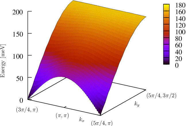
This Hamiltonian describes three two-fold degenerate modes , which we have plotted assuming as cuts along and in Fig. 9. The two-fold degeneracy of each mode corresponds to spin waves with . Since we expect our spin wave theory to be reliable only for energies up to , we will disregard the higher modes along with those analyzed in Appendix C. The lowest mode is shown as a 3D plot for half of the reduced Brillouin zone in Fig. 10.
The Hamiltonian (54) further contains a contribution
| (55) |
to the ground state energy. (Here denotes the number of rungs. The sum extends over values for .) In Appendix D, we obtain the ground state energy by adding this contribution to the contributions of the other terms in (26) given in Appendix C, and obtain . We find that this number is in excellent agreement with what we would expect from diagonalizing the model for a finite cluster with unfrustrated boundary conditions. This confirms the validity of our analysis.
VI Discussion of the results
VI.1 Agreement with the experimental data
The significance of our results emerges in the context of a comparison of our spectrum with the experimental data obtained by Tranquada et al. [15] through inelastic neutron scattering on the stripe ordered compound La1.875Ba0.125CuO4. The data points with their corresponding error bars are shown as black or blue crosses in Figs. 1a and 1b, respectively.
In Fig. 1b, which is directly reproduced from Tranquada et al.[15], the neutron data are superposed with the spectrum of the triplet excitation of an isotropic two-leg Heisenberg ladder, which models bond centered stripes at accordingly high energies. In Fig. 1a, we have superposed cuts of the lowest mode along and with the experimental data. (The superposition of cuts of our spectrum in the and direction reflects the assumption that a superposition of domains with stripes along the two principal lattice directions has been observed in the experiment.) We believe it is fair to say that up to energies of about , the agreement is excellent. (Above these energies, or more precisely above energies of order , a perturbative spin wave analysis becomes unreliable.) Likewise, the constant energy slices of the neutron scattering intensities obtained with the matrix elements calculated in Appendix E shown in Fig. 11 agree very well with the experimentally measured constant-energy slices of the magnetic scattering in La1.875Ba0.125CuO4 shown in Fig. 2 of Tranquada et al.[15].


VI.2 Dependence on the inter-ladder coupling
The good agreement of our results with the experimental data up to energies even larger than (where we would expect that the perturbative spin wave analysis becomes unreliable) is somewhat surprising. While any explanation in terms of bond-centered stripes through coupled two-leg ladders[15, 23, 24] gives immediately a roughly adequate estimate for the saddle-point energy in terms of the triplet energy gap of the individual two-leg ladders, it is far from obvious that a model of coupled three-leg ladders, which are individually gapless, should give a saddle-point energy consistent with the data. In our model, the saddle-point energy depends significantly on the coupling between the ladders. Fortunately, however, it is possible to determine rather accurately through numerical comparison of a – model with a site centered spin and a site centered charge stripe to a model with three-leg Heisenberg ladders coupled by , as described in Appendix B. This analysis does not only provide us with the value , but also shows that this value is rather robust in the sense that it does not significantly depend on the details of how we localize the stripe. To obtain a better understanding of the dependence of our final results on this coupling, we have obtained the spectrum for a number of different values of by solving (21) numerically for each value, and proceeding with the Bogoliubov transformation with the resulting values for and . The results for the saddle-point energies are shown in Fig. 12 (black dots). Fitting the data yields
| (56) |
to an excellent approximation up to values where becomes comparable to (solid line).

The square root dependence of on can be understood by considering a model of two three-leg ladders, which are weakly coupled by , as shown in Fig. 13a. The low energy excitations of the individual three-leg ladders are spin spinons, which are gapless. The coupling induces a linear confinement potential
| (57) |
between pairs of spinons, since the links coupling the chains effectively become decorrelated in the region between them. The situation here is similar to a system of two coupled spin chains shown in Fig. 13b, where a weak coupling between the chains is known to induce a linear confinement potential between pairs of spinons [18]. In the model of coupled chains, the force between the spinons is proportional to[38, 19]
| (58) |
For the model of two coupled three-leg ladders we consider here in the context of understanding the dependence (56) of our spin wave analysis, however, we assume that the spin correlation between the sites coupled by is to lowest order independent of . Therewith we account for the static correlations present due to the long range order we assume. For the confinement force in our auxiliary model of two coupled three-leg ladders we hence assume
| (59) |
The spinon confinement will then induce a gap , which corresponds to the the ground state or zero-point energy of the linear potential oscillator for the relative motion of the spinons. The dispersion of the spinons is linear for both the individual spin chains and the individual three-leg ladders[39],
| (60) |
with as is the only energy scale is these models. (In (60), we have shifted both spinon branches to the origin.) The ground state energy of a constant force oscillator of linearly dispersing particles with velocity , however, is proportional to [40]. This implies for the two weakly coupled chains and for the two weakly coupled three-leg ladders with the additional assumption of static correlations sue to long range order.
To see why this gap corresponds to the saddle point energy in the spin wave analysis above, consider the transformation properties of our auxiliary model of the two weakly coupled three-leg ladders shown in Fig. 13a under the parity reflection . The gapped spinon-spinon bound state is odd under this symmetry, which in the language of momenta of the site centered stripe model corresponds to a shift of . Since the ground state of the stripe model has order with , the gapped excitation will correspond to . Following this line of reasoning, we can understand the square root dependence (56) of depicted in Fig. 12.
VII Conclusions
In this work, we have provided a full and detailed account of a spin wave analysis of a coupled three-leg ladder model for spin stripes in copper oxide superconductors. We have numerically evaluated the inter-ladder coupling induced by the charge stripes in between both site-centered spin stripes modelled by three-leg ladders and bond-centered spin stripes modelled by two-leg ladders. As reported previously [35], for the latter we obtain a ferromagnetic coupling , which is not sufficient to close the energy gap of the individual two-leg ladders. This does not imply that the stripes cannot be bond-centered. It does imply, however, that a description in terms of spin-only models of coupled two-leg ladders is not sensible.
For site-centered spin stripes modelled by three-leg ladders, we
obtain an antiferromagnetic coupling . We have calculated
the spectrum, the staggered magnetization, the dynamical structure
factor , and the ground state energy for a
spin-only model of coupled three-leg ladders using a linear spin wave
analysis of bosonic operators representing the eight-dimensional
Hilbert spaces on each three-site rung. The analysis makes no
assumptions except for the model itself, and contains no variational
parameter, as even the inter-ladder coupling is evaluated through
exact diagonalizations of small – clusters with and without
charge stripes in between the spin stripes. We find excellent
agreement with the experimental data of Tranquada
et al. [15]. The experimental data hence point
towards site-centered, and not, as previously asserted,
bond-centered [15, 23, 24]
stripes.
ACKNOWLEDGMENTS
We wish to thank Matthias Vojta, Tobias Ulbricht, and Peter Wölfle for discussions of this work. This work was supported by the German Research Foundation under grant FOR 960.
Appendix A Matrix elements of the individual spin operators on rungs
Appendix B Estimation of the coupling between ladders
The effective, antiferromagnetic coupling between neighboring spin stripes described by three-leg ladders is induced by the charge stripes between the ladders, since an antiferromagnetic alignment of the spins on each side of the charge stripe enhances the mobility of the holes. To determine this coupling, we have exactly diagonalized 16 site clusters of itinerant spin 1/2 antiferromagnets described by the – model[3, 4] with , two holes, and periodic boundary conditions (PBCs), in which the spin stripes are localized. The Hamiltonian is given by
| (71) | |||||
where the first two sums extend over all nearest-neighbor pairs , and denotes a staggered magnetic field, as indicated by the signs in Fig. 14. The Gutzwiller projector P eliminates doubly occupied sites.

| Site-centered stripe models | |||
|---|---|---|---|
| PBCs | unfrustrated | frustrated | |
| as in | Fig. 14a | Fig. 14b | |
| – model with spin and charge stripes | |||
| , , , , 2 holes | |||
| -21.3409 | -21.2405 | 0.1004 | |
| -0.5415 | |||
| -0.3140 | |||
| 0.2411 | |||
| 0.9437 | |||
| 0.8781 | |||
| three-leg Heisenberg ladder with coupling | |||
| , , , | |||
| -8.0068 | -7.9065 | 0.1003 | |
We compare the ground state energies we obtain for clusters with unfrustrated PBCs shown in Fig. 14a with the ground state energies we obtain for clusters with frustrated PBCs shown in Fig. 14b, in which the 16-site unit cells on the right are shifted by one lattice spacing to the top. We then consider spin-only Heisenberg models of three-leg ladders, which consist of only the sites in the shaded areas in Figs. 14a and 14b, subject to the same staggered field , and couple them antiferromagnetically by , as indicated. The Heisenberg models are described by
| (72) |
where for all nearest-neighbor links inside the shaded areas, but for nearest-neighbor links across the horizontal boundary lines between those areas. We again compare the ground state energies for unfrustrated PBCs, where couples sites 10 and 1, 11 and 2, etc. for the three-leg ladders shown in the shaded areas in Fig. 14a, with frustrated PBCs, where couples sites 11 and 1, 12 and 2, etc. , as shown in Fig. 14b. Finally, we determine such that the difference in the ground state energies between frustrated and unfrustrated PBCs in the – clusters matches this difference in the spin-only ladder models.
With we obtain , as detailed in Tab. 1. The value for is chosen self-consistently such that the mean value of the staggered magnetization we obtain for our spin wave theory in Appendix F,
| (73) |
matches the corresponding value in the – cluster shown in Fig. 14a. For this cluster, however, there are two values for the staggered magnetization, depending on whether we consider the overall magnetization
| (74) |
or the magnetization on only those sites which are occupied by electrons (which differs since the holes are not strictly localized on the chain in between the shaded areas in Fig. 14b):
| (75) |
We assert that these two values constitute lower and upper bounds of what we would expect in a spin-only model, and chose such that the spin wave theory gives the mean value of these bounds (this value is 0.2906).

| Bond-centered stripe models | |||
|---|---|---|---|
| PBCs | unfrustrated | frustrated | |
| as in | Fig. 15a | Fig. 15b | |
| – model with spin and charge stripes | |||
| , , , , 2 holes | |||
| -21.3428 | -21.2526 | 0.0902 | |
| -0.5395 | |||
| two-leg Heisenberg ladder with coupling | |||
| , , , | |||
| -5.1557 | -5.0655 | 0.0902 | |
For completeness, we also provide the details of the corresponding calculation for the effective coupling between bond-centered stripes modelled by two-leg ladders, in Tab 2. The calculation differs only in that we now use the finite size clusters depicted in Figs. 15a and 15b. The value of the staggered magnetic field is chosen such that the staggered magnetic field energy described by the last term in (71) is equal to the value we obtained for the three-leg ladder model listed in see Tab. 1. We obtain a ferromagnetic coupling . This value is not large enough to close the spin gap of the the individual two-leg ladders, and hence precludes a description of bond-centered stripes in terms of spin-only models of coupled two-leg ladders[35].
It should be born in mind that the values we obtain here are only estimates, as it is impossible to calculate a precise value for a coupling between spin-only models of stripes, as these constitute a rather crude approximation themselves. We are confident, however, that the coupling for three-leg ladders modelling site-centered stripes is between and , and that the absolute value of the coupling between two-leg ladders describing bond-centered stripes is significantly smaller than this coupling.
Appendix C Analysis of , , , , and
In this appendix, we expand and analyze the terms in the Hamiltonian (26) which have no influence on the low energy spectrum in this appendix. These terms, however, are required for evaluations of the ground state energy.
C.1 The bare ground state energy
The bare ground state energy accounts for the constant terms in the Hamiltonian (17). It is given by with
| (76) | |||||
C.2 Evaluation of the spectrum of
The term is given by
| (77) | |||||
with
To a reasonable approximation, we obtain low energy modes described by by diagonalizing (77) at each point in space in the reduced Hilbert space spanned by
where
| (80) |
is the bare vacuum unrenormalized by spin wave theory. This yields two almost dispersionless modes
| (81) |
with energies of about , or if we assume . Cuts of the dispersions of these two modes are shown in blue (color online) in Fig. 16. also gives rise to a contribution
| (82) |
to the ground state energy. (Here denotes the number of rungs, which implies that the sum extends over values for .)

C.3 Evaluation of the spectrum of
A similar analysis of
| (83) | |||||
with
| (84) | |||||
yields two additional, almost dispersionless modes
| (86) |
with energies of about , or , which is shown in green (color online) in Fig. 16. also gives rise to a contribution
| (87) |
to the ground state energy.
C.4 Evaluation of the spectrum of
The term
| (88) | |||||
with as given in (C.2) and
can be diagonalized by a Bogoliubov transformation. We obtain
| (90) |
with
| (91) |
It yields a two-fold degenerate, weakly dispersing mode with an energy of about , or , which is shown in red (color online) in Fig. 16, as well as a contribution
| (92) |
to the ground state energy.
C.5 Evaluation of the spectrum of
Finally,
| (93) |
with
| (94) | |||||
describes a two-fold degenerate, completely dispersionless mode with an energy of , or .
Appendix D Ground state energy
To evaluate the ground state energy , we collect the contributions from (76), (82), (87), (92), and (). This yields
| (95) |
where is the number of rungs. This number is in good agreement with what we would expect from the results of exact diagonalizations of
| (96) |
for small clusters of 12, 18 and 24 sites with unfrustrated boundary conditions, as shown for rungs by the shaded areas in Fig. 14a. Specifically, we obtain for a cluster with rungs, , and unfrustrated boundary conditions with a shift of 3 lattice spacings. If we compare the nearest-neighbor spin-spin correlation we obtain from exactly diagonalizing the same 24 site cluster with , , to the the value predicted by standard two-dimensional linear spin wave theory[41], , we are led to estimate that the bond operator spin wave theory developed here should yield a number around
| (97) |
This differs only by 1% from (95).
Appendix E Matrix Elements
The dynamical structure factor measured in neutron scattering is given by
| (98) |
where is the ground state and the sum extends over all excited states with energy , and
| (99) |
is the Fourier transform of the spin raising operator at lattice site with respect to original lattice, i.e., the sum runs over all lattice sites. This implies
| (100) | |||||
| (101) |
with and as indicated in Fig. 7 for sublattices and , respectively. In analogy to Fourier transforms of the bosonic creation and annihilation operators (23) and (24), we further Fourier transforms of the spin operators with respect to the rung sublattices and according to
| (102) | |||||
| (103) |
and express the operator (99) in terms of them:
| (104) | |||||

As we are interested only in the contribution of the low-energy mode to , the only matrix element we need to evaluate is
| (105) |
for all values of . (The second low-energy mode , which is degenerate with the first, does not contribute to (105) and hence to , but instead yields a contribution to which is identical to the one we calculate below.) Keeping only terms which contribute to this mode and are linear in the expansion (14) of , we obtain for sublattice
or in Fourier space with (102), (23), and (28)
| (106) | |||||
and similarly with (16) and (24) for
| (107) | |||||
We then use and (53) to express and in terms of and , recall , and finally obtain
Note that as there is no term linear in
, , or in the expansion (14)
for .
Appendix F Staggered magnetization
The staggered magnetizations on the outer and inner chains of our three-leg ladders, and , respectively, are given in by the the bare values with minus corrections from the individual terms in the Hamiltonian (26). From (68)–(70) with (22), we obtain for the bare values
| (109) | |||||
| (110) |
We expect that the largest corrections arise from , as this part contains the only low energy mode of the theory. The for this part relevant terms in the expansion (14) for are
| (111) |
For convenience, we define
| (112) | |||||
and express the operators as well as their hermitian conjugates via through the operators (see (28)), (44), and (53) above). Using and , we obtain for the corrections from
In this sum, the terms in the first pair of square brackets originate from the low energy eigenmodes in the energy range from 0 to about 190 meV in Fig. 9, the terms in the second pair originate form at about 290 meV, and the terms in the third pair originate from at about 460 meV. Evaluation yields
| (113) | |||||
| (114) | |||||
for the outer and inner chains, respectively. As expected, the low energy mode we compare to the experiment[15] yields the dominant contribution.
The corrections arising from are evaluated in complete analogy. The Bogoliubov transformation with is now only two-dimensional, and the only contribution comes from the term in (14):
| (115) |
Evaluation yields
| (116) | |||||
| (117) |
References
- [1] J. Zaanen et al., Nature Physics 2, 138 (2006).
- [2] J. Orenstein and A. J. Millis, Science 288, 468 (2000).
- [3] F. C. Zhang and T. M. Rice, Phys. Rev. B 37, 3759 (1988).
- [4] H. Eskes and G. A. Sawatzky, Phys. Rev. Lett. 61, 1415 (1988).
- [5] H. F. Fong, B. Keimer, P. W. Anderson, D. Reznik, F. Doğan, and I. A. Aksay, Phys. Rev. Lett. 75, 316 (1995).
- [6] P. Bourges, Y. Sidis, H. F. Fong, L. P. Regnault, J. Bossy, A. Ivanov, and B. Keimer, Science 288, 1234 (2000).
- [7] J. Zaanen and O. Gunnarsson, Phys. Rev. B 40, 7391 (1989).
- [8] M. Kato, K. Machida, H. Nakanishi, and M. Fujita, J. Phys. Soc. Jpn. 59, 1047 (1990).
- [9] J. M. Tranquada, B. J. Sternlieb, J. D. Axe, Y. Nakamura, and S. Uchida, Nature 375, 561 (1995).
- [10] V. J. Emery, S. Kivelson, and J. Tranquada, Proc. Natl. Acad. Sci. U.S.A. 96, 8814 (1999).
- [11] J. Zaanen, O. Y. Osman, H. V. Kruis, Z. Nussinov, and J. Tworzydło, Phil. Mag. B 81, 1485 (2001).
- [12] H. A. Mook, P. Dai, and F. Doğan, Phys. Rev. Lett. 88, 097004 (2002).
- [13] S. A. Kivelson, I. P. Bindloss, E. Fradkin, V. Oganesyan, J. M. Tranquada, A. Kapitulnik, and C. Howald, Rev. Mod. Phys. 75, 1201 (2003).
- [14] E. Berg, E. Fradkin, S. A. Kivelson, and J. Tranquada, New J. Phys. 11, 115004 (2009).
- [15] J. Tranquada, H. Woo, T. Perring, H. Goka, G. Gu, G. Xu, M. Fujita, and K. Yamada, Nature 429, 534 (2004).
- [16] B. Fauqué, Y. Sidis, L. Capogna, A. Ivanov, K. Hradil, C. Ulrich, A. I. Rykov, B. Keimer, and P. Bourges, Phys. Rev. B 76, 214512 (2007).
- [17] E. Dagotto and T. M. Rice, Science 271, 618 (1996).
- [18] D. G. Shelton, A. A. Nersesyan, and A. M. Tsvelik, Phys. Rev. B 53, 8521 (1996).
- [19] M. Greiter, Phys. Rev. B 66, 054505 (2002).
- [20] G. Xu, J. M. Tranquada, T. G. Perring, G. D. Gu, M. Fujita, and K. Yamada, Phys. Rev. B 76, 014508 (2007).
- [21] V. Hinkov, S. Pailhes, P. Bourges, Y. Sidis, A. Ivanov, A. Kulakov, C. T. Lin, D. P. Chen, C. Bernhard, and B. Keimer, Nature 430, 650 (2004).
- [22] V. Hinkov, P. Bourges, S. Pailhès, Y. Sidis, A. Ivanov, C. D. Frost, T. G. Perring, C. T. Lin, D. P. Chen, and B. Keimer, Nature Physics 3, 780 (2007).
- [23] M. Vojta and T. Ulbricht, Phys. Rev. Lett 93, 127002 (2004).
- [24] G. S. Uhrig, K. P. Schmidt, and M. Grüninger, Phys. Rev. Lett 93, 267003 (2004).
- [25] V. I. Anisimov, M. A. Korotin, A. S. Mylnikova, A. V. Kozhevnikov, D. M. Korotin, and J. Lorenzana, Phys. Rev. B 70, 172501 (2004).
- [26] S. Sachdev and R. N. Bhatt, Phys. Rev. B 41, 9323 (1990).
- [27] F. Krüger and S. Scheidl, Phys. Rev. B 67, 134512 (2003).
- [28] R. Eder, Phys. Rev. B 57, 12832 (1998).
- [29] S. Gopalan, T. M. Rice, and M. Sigrist, Phys. Rev. B 49, 8901 (1994).
- [30] J. Tworzydło, O. Y. Osman, C. N. A. van Duin, and J. Zaanen, Phys. Rev. B 59, 115 (1999).
- [31] S. Dalosto and J. Riera, Phys. Rev. B 62, 928 (2000).
- [32] T. S. Nunner, P. Brune, T. Kopp, M. Windt, and M. Grüninger, Phys. Rev. B 66, 180404(R) (2002).
- [33] G. Seibold and J. Lorenzana, Phys. Rev. Lett. 94, 107006 (2005).
- [34] G. Seibold and J. Lorenzana, Phys. Rev. B 73, 144515 (2006).
- [35] M. Greiter and H. Schmidt, Phys. Rev. B 82, 144512 (2010).
- [36] D. X. Yao, E. W. Carlson, and D. K. Campbell, Phys. Rev. Lett. 97, 017003 (2006).
- [37] S. Sachdev, Phys. Rev. B 45, 12377 (1992).
- [38] M. Greiter, Phys. Rev. B 65, 134443 (2002).
- [39] T. M. Rice, S. Haas, M. Sigrist, and F.-C. Zhang, Phys. Rev. B 56, 14655 (1997).
- [40] M. Greiter, Ann. Phys. 325, 1349 (2010).
- [41] P. W. Anderson, Phys. Rev. 86, 694 (1952).