Light bending by nonlinear electrodynamics under strong electric and magnetic field
Abstract
We calculate the bending angles of light under the strong electric and magnetic fields by a charged black hole and a magnetized neutron star according to the nonlinear electrodynamics of Euler-Heisenberg interaction. The bending angle of light by the electric field of charged black hole is computed from geometric optics and a general formula is derived for light bending valid for any orientation of the magnetic dipole. The astronomical significance of the light bending by magnetic field of a neutron star is discussed.
pacs
12.20.Fv,41.20.Jb,95.30-kI Introduction
A nonuniform electric or magnetic background field can induce a continually varying index of refraction. At classical level the linearity of the electrodynamics precludes the bending of light by electric or magnetic field. Therefore any bending must involve a nonlinear interaction from quantum correction. Because of the nonlinear optical properties by Euler-Heisenberg interaction [1, 2] arising from the box diagram of quantum electrodynamics, the light can bend when it passes the neighborhood of an electrically or magnetically charged object.
Since the maximum available field in a laboratory is of the order , it is difficult to observe the bending directly in a laboratory [3, 4, 5, 6, 7]. An alternative way one can think of is observing the effect in the astronomical scale. There are objects, at least considered theoretically, with electric or magnetic field strong enough to make such bending relevant. One example of light bending by an electrically charged object is when a high energy photon passes around a charged black hole with impact parameter greater than the Schwarzschild radius [8]. Another example of light bending by a magnetic field is when a photon passes the magnetosphere of a magnetized neutron star with extremely strong magnetic field of the order . Since neutron stars have a very dense magnetosphere, only high energy photons may be observable. Recently the vacuum effect of non-linear electrodynamics under strong magnetic field by magnetized stars has been studied widely [9, 10, 11, 12, 13, 14, 15, 16, 17, 18, 19, 20, 21].
We will calculate the bending angle of the incident photon under the electric and magnetic field. In the previous work of the authors, we set up a simple formalism to find the bending angle and the trajectory of light in a Coulombic field at atomic scale [22]. In this paper, we consider the bending of a high energy photon when it passes near an astronomical object with strong electric or magnetic field. The organization of the paper is as follow. In Sec. II, we set up the trajectory equation to calculate the bending angle based on Euler-Heisenberg interaction. In Sec. III, we consider the bending by the electric field of a spherically symmetric charged object. In Sec. IV, we consider the bending by the magnetic field of a magnetic dipole. We derive a general formula valid for any orientation of the dipole axis and discuss some special cases where the dipole axis and the beam direction are aligned in a particular way. Finally, in Sec. V, we conclude and discuss the possibility of observation.
II The trajectory equation
The nonlinear interaction of photons is described by the Euler-Heisenberg Lagrangian [1, 2]
| (1) | |||||
In the presence of the electric field, the correction to the speed of light due to the nonlinear interaction is [23, 24, 25, 26, 27, 28, 29, 30, 31, 32, 33]
| (2) |
where denotes the unit vector in the direction of photon propagation, for the perpendicular mode in which the photon polarization is perpendicular to the plane spanned by and , and for the parallel mode where the polarization is parallel to the plane. Throughout the paper all units are in MKS. For magnetic case, should be replaced by in the above equation. Because the speed of light depends on the electric field the light ray bends in the presence of a nonuniform field. The bending can be calculated by geometric optics. The index of refraction due to the background field is given, in the leading order, by
| (3) |

The infinitesimal bending of the photon trajectory over can be obtained from the Snell’s law as
| (4) |
where and denotes the angle between and (see Fig. 1). Since light bends in general toward the direction of greater index of refraction we can write the bending in a vector form
| (5) |
which leads to the trajectory equation
| (6) |
where denotes the distance parameter of the light trajectory with and
| (7) |
Since the correction to the index of refraction is generally small in our consideration the trajectory equation can be approximated to the leading order as
| (8) |
where denotes the initial direction of the incoming photon. Throughout the paper we shall assume the photon comes in from and moves to direction, hence
| (9) |
and putting the trajectory equation becomes
| (10) |
The first equation shows that at leading order, which is obviously true, and therefore the trajectory equations for and in the perpendicular directions to the incoming photon are given by
| (11) |
which will be used in the following analysis.
III Bending by spherically symmetric charged object
We now consider the bending of photon trajectory by a spherically symmetric charged object of total charge . For this case the bending angle can be calculated in the same way as in Coulombic case with the electric field
| (12) |
For a photon trajectory moving to axis in the plane, choose the unit vector in the direction of photon propagation as
| (13) |
where prime is the derivative with respect to . The index of refraction can be written as
| (14) |

For a photon incoming from with impact parameter (see Fig. 2), the initial condition reads
| (15) |
and from the first of the trajectory equation (11)
| (16) |
where is the Compton length of the electron. The total bending angle can be obtained by integration
| (17) |
By putting in , for the leading order solution, we obtain
| (18) |
The bending always occurs toward the center of the charged object as in the bending by gravitational field.
To compare the bending by electric field with the bending by gravitation, let us consider a charged non-rotating black hole with mass and charge . The bending by gravitational field is well-known
| (19) |
Note that, from and , the bending by electric field can be important at short distance. The charge and angular momentum per unit mass() is constrained by the mass of the black hole, in Planck units, as [34]
| (20) |
For non-rotating () charged black hole, restoring the physical constants, the total electric charge is constrained by the condition
| (21) |
We can parameterize the charge as
| (22) |
with . Then the magnitude of the bending angle by electric field can be written as
| (23) |
To estimate the size of the bending, let us compare the two bending angles for the maximally charged (extremal, ) stellar black hole of ten solar mass . Since our formalism is based on flat space time, not on general relativity, the impact parameter should be large enough. We consider the case when the impact parameter is ten times the Schwarzschild radius, , at which
| (24) |
The bending by electric charge dominates the gravitational bending. Even for non-extremal charged black hole with , the electrical bending, , is comparable to the gravitational bending.
This example shows that the bending by electric field can be large. However, it may not survive the screening by electron-positron pair creations of the strong electric field. As well known, as the electric field strength approaches the QED critical field
| (25) |
the electric field is susceptible to electron-positron pair creation. In the region where the electric field is of the order or higher than , the vacuum is unstable and the electric field is highly screened by the pair creation [2, 35]. Only photons entering the region with electric field below can have a chance to be observed.
To simplify the discussion we may write (23) as
| (26) |
where is the ratio of the black hole mass to the solar mass,
| (27) |
is the Coulomb field at radius :
| (28) |
with given by (22), and denotes the radius at which given by
| (29) |
where is the Schwarzschild radius of the black hole . Eq. (26) shows that at , for which the electric field strength is below , the ratio is bounded by
| (30) |
which shows that the screening by pair creation severely bounds the valid range of the bending angle by a black hole with mass larger than the solar mass. The light bending can be comparable to the gravitational bending only for black holes with mass substantially smaller than the solar mass.

IV Bending by magnetic dipole
We consider the bending of photon trajectory by a magnetic dipole. Obviously, the bending by magnetic dipole should depend on the orientation of dipole relative to the direction of the incoming photon. We consider the bending by a magnetic dipole located at the origin with arbitrary orientation (see Fig. 3). We take the direction of the incoming photon as axis, horizontal direction as axis, and vertical direction as axis. For the magnetic dipole located at origin, we define the directional cosines , , such that . The magnetic field by the dipole is given by
| (31) |
and the index of refraction due to this background magnetic field is
| (32) |
Taking the unit vector in the direction of photon propagation as
| (33) |
the index of refraction can be written as
| (34) |
To the leading order, the index of refraction is written explicitly as
| (35) | |||||
and from the photon trajectory equation (11) we have
| (36) | |||||
| (37) | |||||
The total bending angle can be obtained by integration by putting and in (36) and (37), which gives for horizontal () and vertical () deflections,
| (38) | |||||
| (39) |
An important comment is in order. The result is valid as long as the polarization of the photon remains, throughout the trajectory, perpendicular or parallel to the plane spanned by and . It can be easily checked that this condition is met only when the magnetic dipole axis is either in direction or in the plane. When the dipole axis is in none of these directions the photon polarization remains neither in pure perpendicular nor in pure parallel mode, even if it started in one of the modes. In this case the birefringence effect takes place, and the perpendicular and the parallel modes of the light ray split. Since the splitting occurs continually on every branch-out rays, this cascade of splitting results in the initial single light ray branching out to a light bundle. The bending angles (38) and (39), with either 14 for the perpendicular mode or 8 for the parallel mode, then provide an envelope for the maximal and minimal bending angles of the light bundle in the horizontal and perpendicular direction, respectively.

Let us now consider some special cases which will allow us to compare our result with the previous work. First, we consider the case when the photon path is perpendicular to the dipole moment and traveling on the equator of the dipole. Assume that the magnetic moment directs along and the incident photon is coming from (see Fig. 4). This is the specific case considered by Denisov et al. [11]. Taking and , the magnetic field on the dipole equator ( plane) is given by
| (40) |
By symmetry, there is no vertical () bending, so , and the horizontal () bending angle is given by
| (41) |
This result agrees with Denisov et al. (see the Eqs. (4) and (5) in [11]).

Second, consider the case when the photon path is parallel or anti-parallel to the dipole axis. Assume that the dipole at the origin directs along the axis in the plane (see Fig. 5). Taking and , the magnetic field on the plane is given by
| (42) |
Also there is no bending in direction, , and the bending angle in direction is given by
| (43) |

Finally, consider the case when the photon path is perpendicular to dipole moment and passes the north or south pole. Locate the dipole at the origin directing along the axis in the plane (see Fig. 6). Taking and , the magnetic field on the plane is given by
| (44) |
There is also no vertical bending, , and the horizontal bending angle is given by
| (45) |
This configuration gives the maximum possible bending; The gradient of index of refraction is maximal along this direction.
Let us now compare the bending by magnetic field with the gravitational bending. We will consider the possible maximum bending given by Eq. (45) for a strongly magnetized neutron star with solar mass and radius . For extremely strongly magnetized neutron stars the magnetic field at the surface can be strong as . Parameterizing the impact parameter in units of the radius with , the bending by a magnetic field can be written as
| (46) |
where we have used , the magnetic field strength at the neutron star surface. For the magnetic field strength of of a neutron star, the maximum value of the bending angle is given by
| (47) |
which is for a ray glancing the north or south pole where the bending is maximal. This is much smaller than the gravitational bending .
By increasing the surface magnetic field a larger bending angle can be obtained. However, as in the bending by charged black hole, the bending is constrained by the screening of electron-positron pair creation of strong magnetic field above the critical strength
| (48) |
To see this we may write (46) as
| (49) |
where is the magnetic field at radius given by
| (50) |
and denotes the Schwarzschild radius . To avoid the screening we require , which gives the bound
| (51) |
where denotes the radius at which . Thus, a larger bending can be obtained with large , but it is obviously bounded by the surface magnetic field strength through the relation
| (52) |
For a magnetar with , for example, we get , and considering that the magnetic bending is expected to be, at most, a few percent of the gravitational bending.
V Discussion
We have studied how photons can be bent when they travel through the strong electric or magnetic field of compact object like a charged black hole or a neutron star. We calculated the bending angles according to the nonlinear electrodynamics of Euler-Heisenberg interaction. Our calculation shows that the bending by electrically charged astronomical object can be comparable or larger than the gravitational bending. However, the screening by the electron-positron pair creation strongly bounds the electric bending so that the electric bending can be significant compared with the gravitational bending only for black holes with mass substantially smaller than the solar mass. We also found a general formula for light bending by magnetic field, valid for any orientation of the magnetic dipole. Our calculation shows that for a magnetar with surface magnetic field the magnetic bending can be, at most, a few percent of the gravitational bending.
Since the magnetic bending is expected to be small compared to gravitational bending any chance of observation may be realized only when the experiment detects the small variation over the gravitational bending. One way to observe the light bending by magnetic field may be using the birefringence [9] that the bending of perpendicular polarization is 1.75(=14/8) times larger than the bending of parallel polarization. Even in the region where the bending by magnetic field is weak compared with the gravitational bending, by eliminating the overall gravitational bending, the polarization dependence of the bending by magnetic field may be tested if the allowed precision is sufficient enough.
Another possibility is detecting the time variation in bending. The magnetic axis of a magnetar is likely to be different from the rotational axis. In this case the magnetic bending by a rapidly spinning magnetar will add a small wiggling effect over the gravitational bending.
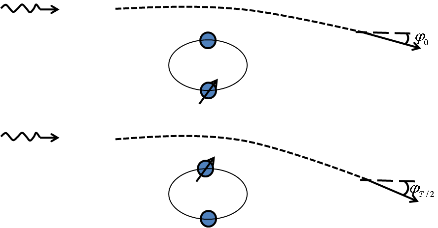
The neutron star in a binary system [19] may also be used to detect the magnetic bending. Most of the neutron stars are isolated stars, less than one hundred are known to be in binary systems with nondegenerate stars. Assume for simplicity that the nondegenerate companion star has the same mass as the neutron star. If we consider only the bending by gravitation, the bending at and the bending at a half orbital period later will be the same. However, when the bending by magnetic field is included, the bending angles will be different by the relative position of the two stars (see Fig. 7).
Acknowledgements.
We would like to thank Y. Yi, M. I. Park, and M. K. Park for useful discussions. This paper was supported by research funds of Kunsan National University.References
- [1] W. Heisenberg and H. Euler, Z. Phys. 98, 714 (1936), physics/0605038.
- [2] J. S. Schwinger, Phys. Rev. 82, 664 (1951).
- [3] E. Iacopini and E. Zavattini, Phys. Lett. B 85, 151 (1979).
- [4] D. Bakalov et al., Nucl. Phys. B 35 (Proc. suppl.), 180 (1994).
- [5] D. Boer and J.-W van Holten, hep-ph/0204207.
- [6] A. Di Piazza, K. Z. Hatsagortsyan, and C. H. Keitel, Phys. Rev. Lett. 97, 083603 (2006).
- [7] B. King, A. Di Piazza, and C. H. Keitel, Nature Photon. 4, 92 (2010).
- [8] V. A. De Lorenci, N. Figueredo, H. H. Fliche, and M. Novello, Astron. Astrophys. 369, 690 (2001).
- [9] N. J. Shaviv, J. S. Heyl, and Y. Lithwick, Mon. Not. R. Astron. Soc. 306, 333 (1999).
- [10] J. S. Heyl and N. J. Shaviv, Mon. Not. R. Astron. Soc. 311, 555 (2000).
- [11] V. I. Denisov, I. P. Denisova, and S. I. Svertilov, Dokl. Akad. Nauk. Ser. Fiz. 380, 435 (2001).
- [12] V. I. Denisov, I. P. Denisova, and S. I. Svertilov, Dokl. Phys. 46, 705 (2001).
- [13] J. S. Heyl and N. J. Shaviv, Phys. Rev. D 66, 023002 (2002).
- [14] V. I. Denisov and S. I. Svertilov, Astron. Astrophys. 399, L39 (2003).
- [15] J. S. Heyl, N. J. Shaviv, and D. Lloyd, Mon. Not. R. Astron. Soc. 342, 134 (2003).
- [16] V. I. Denisov, I. P. Denisova, and S. I. Svertilov, Theor. Math. Phys. 140, 1001 (2004).
- [17] V. I. Denisov and S. I. Svertilov, Phys. Rev. D71, 063002 (2005).
- [18] J. S. Heyl, D. Lloyd, and N. J. Shaviv, astro-ph/0502351.
- [19] A. Dupays, C. Robilliard, C. Rizzo, and G. F. Bignami, Phys. Rev. Lett. 94, 161101 (2005).
- [20] P. A. Vshivtseva, V. I. Denisov, and I. V. Krivchenkov, Theor. Math. Phys. 150, 73 (2007).
- [21] D. Mazur and J. S. Heyl, Mon. Not. R. Astron. Soc. 412, 1381 (2011).
- [22] J. Y. Kim and T. Lee, Mod. Phys. Lett. A 26, 1481 (2011).
- [23] Z. Bialynicka-Birula and I. Bialynicka-Birula, Phys. Rev. D 2, 2341 (1970).
- [24] S. L. Adler, Annals Phys. 67, 599 (1971).
- [25] J. S. Heyl and L. Hernquist, J. Phys. A 30, 6485 (1997).
- [26] H. Gies and W. Dittrich, Phys. Lett. B 431, 420 (1998).
- [27] W. Dittrich and H. Gies, Phys. Rev. D 58, 025004 (1998); hep-ph/9806417.
- [28] J. S. Heyl and L. Hernquist, Phys. Rev. D 58, 043005 (1998).
- [29] M. Novello, V. A. De Lorenci, J. M. Salim, and R. Klippert, Phys. Rev. D 61, 045001 (2000).
- [30] V. A. De Lorenci, R. Klippert, M. Novello, and J. M. Salim, Phys. Lett. B 482, 134 (2000).
- [31] H. Gies, hep-ph/0010287.
- [32] G. L. J. A. Rikken and C. Rizzo, Phys. Rev. A 63, 012107 (2001).
- [33] V. A. De Lorenci and G. P. Goulart, Phys. Rev. D 78, 045015 (2008).
- [34] C. W. Misner, K. S. Thorne, and J. A. Wheeler, Gravitation (W. H. Freeman and Company, New York) (1970).
- [35] C. Itzykson and J.-B. Zuber, Quantum field theory (McGraw Hill) (1980).