Multi-Stage Improved Route Planning Approach
Abstract
A new approach to the static route planning problem, based on a multi-staging concept and a scope notion, is presented. The main goal (besides implied efficiency of planning) of our approach is to address—with a solid theoretical foundation—the following two practically motivated aspects: a route comfort and a very limited storage space of a small navigation device, which both do not seem to be among the chief objectives of many other studies. We show how our novel idea can tackle both these seemingly unrelated aspects at once, and may also contribute to other established route planning approaches with which ours can be naturally combined. We provide a theoretical proof that our approach efficiently computes exact optimal routes within this concept, as well as we demonstrate with experimental results on publicly available road networks of the US the good practical performance of the solution.
1 Introduction
The single pair shortest path SPSP problem in world road networks, also known as the route planning problem, has received considerable attention in the past decades. However classical algorithms like Dijkstra’s or A* are in fact ”optimal“ in a theoretical sense, they are not well suitable for huge graphs representing real-world road networks having up to tens millions of edges. In such situation even an algorithm with a linear time complexity cannot be feasibly run on a mobile device lacking computational power and working memory.
What can be done better? We focus on the static route planning problem where the road network is static in the sense that the underlying graph and its attributes do not change in time. Thus, a feasible solution lies in suitable preprocessing of the road network in order to improve both time and space complexity of subsequent queries (to find an optimal route from one position to another). However, to what extent such a preprocessing is limited in the size of the precomputed auxiliary data? It is not hard to see that there is always some trade-off between this storage space requirement and the efficiency of queries—obviously, one cannot precompute and store all the optimal routes in advance. See also a closer discussion below.
Related Work.
Classical techniques of the static route planning are represented by Dijkstra’s algorithm [9], A* algorithm [16] and their bidirectional variations [20]. In the last decade, two sorts of more advanced techniques have emerged and become popular. The first one prunes the search of Dijkstra’s or A* algorithms using preprocessed information This includes, in particular, reach-based [15, 12], landmarks [11, 14], combinations of those [13], and recent hub-based labeling [1].
The second sort of techniques (where our approach conceptually fits, too) exploits a road network structure with levels of hierarchy to which a route can be decomposed into. For instance, highway and contraction hierarchies [21, 24, 10], transit nodes [3], PCD [18] and SHARC routing [4, 5] represent this sort. Still, there are also many other techniques and combinations, but—due to lack of space—we just refer to Cherkassky et al. [6], Delling et al. [8, 7], and Schultes [23]. Finally, we would like to mention the interesting notion of highway dimension [2], and the ideas of customizable [1] and mobile [22] route planning.
Our Contribution.
We summarize the essence of all our contribution already here, while we implicitly refer to the subsequent sections for precise definitions, algorithms, proofs, and further details.
First of all, we mention yet another integral point of practical route planning implementations—human-mind intuitiveness and comfortability of the computed route. This is a rather subjective requirement which is not easy to formalize via mathematical language, and hence perhaps not often studied together with the simple precise “shortest/fastest path” utility function in the papers.
-
Intuitiveness and comfort of a route: Likely everyone using car navigation systems has already experienced a situation in which the computed route contained unsuitable segments, e.g. tricky shortcuts via low-category roads in an unfamiliar area. Though such a shortcut might save a few seconds on the route in theory, regular drivers would certainly not appreciate it and the real practical saving would be questionable. This should better be avoided.
Nowadays, the full (usually commercially) available road network data contain plenty of additional metadata which allow it to detect such unreasonable routes. Hence many practical routing implementations likely contain some kinds of rather heuristic penalization schemes dealing with this comfortability issue. We offer here a mathematically sound and precise formal solution to the route comfort issue which builds on a new theoretical concept of scope (Sec. 3).
The core idea of a scope and of scope-admissible routes can be informally outlined as follows: The elements (edges) of a road network are spread into several scope levels, each associated with a scope value, such that an edge assigned scope value is admissible on a route if, before or after reaching , such travels distance less than on edges of higher scope level than . Intuitively, the scope levels and values describe suitability and/or importance of particular edges for long-range routing. This is in some sense similar to the better known concept of reach [15]; but in our case the importance of an edge is to be decided from available network metadata and hence its comfort and intuitive suitability is reflected, making a fundamental difference from the reach concept.
The effect seen on scope admissible routes (Def. 3, 5,6) is that low-level roads are fine “near” the start or target positions (roughly until higher-level roads become available), while only roads of the highest scope levels are admissible in the long middle sections of distant routing queries. This nicely corresponds with human thinking of intuitive routes, where the driver is presumably familiar with neighborhoods of the start and the target of his route (or, such a place is locally accessible only via low-level roads anyway). On contrary, on a long drive the mentally demanding navigation through unknown rural roads or complicated city streets usually brings no overall benefit, even if it were faster in theory.
To achieve good practical usability, too, road network segments are assigned scope levels (cf. Table 1) according to expectantly available metadata of the network (such as road categories, but also road quality and other, e.g. statistical information). It is important that already experiments with publicly available TIGER/Line 2009 [19] US road data, which have metadata of questionable quality, show that the restriction of admissible routes via scope has only a marginal statistical effect on shortest distances in the network.
Furthermore, a welcome added benefit of our categorization of roads into scope levels and subsequent scope admissibility restriction is the following.
-
Storage space efficiency: We suggest that simply allowing to store “linearly sized” precomputed auxiliary data (which is the case of many studies) may be too much in practice. Imagine that setting just a few attributes of a utility function measuring route optimality results in an exponential number of possibilities to which the device has to keep separate sets of preprocessed auxiliary data. In such a case a stricter storage limits should be imposed.
In our approach, preprocessed data for routing queries have to deal only with the elements of the highest scope(s). This allows us to greatly reduce the amount of auxiliary precomputed information needed to answer queries quickly. We use (Sec. 4.1) a suitably adjusted fast vertex-separator approach which stores only those precomputed boundary-pair distances (in the cells) that are admissible on the highest scope level. This way we can shrink the auxiliary data size to less than of the road network size (Table 3) which is a huge improvement. Recall that vertex-separator preprocessing produces a partition of the network graph into moderate-size cells (several thousands of edges, say) such that only (selected) distances between pairs of their boundary vertices are precomputed.
Not to forget, our subsequent routing query algorithm (Sec. 5) then answers quickly and exactly (not heuristically) an optimal route among all scope admissible ones between the given positions. The way we cope with scope admissibility (among other aspects) in a route planning query, using the precomputed auxiliary data, It is briefly summarized as follows.
-
Multi-staging approach: The computation of an optimal route is split into two (or possibly more – with finer network metadata and hierarchical separators) different stages. In the local – cellular, stage, a modification of plain Dijkstra’s algorithm is used to reach the cell boundaries in such a way that lower levels are no longer admissible. Then in the global – boundary, stage, an optimal connection between the previously reached boundary vertices found on the (much smaller) boundary graph given by auxiliary data.
Notice that the cellular stage may possibly cross the boundaries of a few adjacent cells if the start or target is near to them, but practical experiments show that such a case is quite rare. After all, the domain of a cellular stage is a small local neighbourhood, and Dijkstra’s search can thus be very fast on it with additional help of a reach-like parametrization (Def. 8). Then, handling the precomputed boundary graph in the global stage is very flexible—since no side restrictions exist there—and can be combined with virtually any other established route planning algorithm (see Sec. 5). The important advantage is that the boundary graph is now much smaller (recall, in experiments) than the original network size, and hence computing on it is not only faster, but also more working-memory efficient which counts as well for mobile navigation devices.
Paper organization.
After the informal outline of new contributions, this paper continues with the relevant formal definitions—Section 2 for route planning basics, and Section 3 for thorough description of the new scope admissibility concept. An adaptation of Dijkstra for scope is sketched in Sec. 3.1. Then Section 4 shows further details of the road network preprocessing (4.1) and query (5) algorithms. A summary of their experimental results can be found in Tables 3 and 6.
2 Preliminaries
A directed graph is a pair of a finite set of vertices and a finite multiset of edges. The reverse graph of is a graph on the same set of vertices with all of the edges reversed. A subgraph of a graph is denoted by . A subgraph is induced by a set of edges if and ; we then write .
A walk is an alternating sequence of vertices and edges of such that for . A subwalk is a subsequence of a walk. A concatenation of walks and is the walk . If is a single edge , then we write .
A walk is is a prefix of another walk if is a subwalk of starting with the same index, and analogically with suffix. The prefix set of a walk is and analogically . Two walks are overhanging (one another) if either one is a subwalk of the other, or a non-zero-length suffix of one is a prefix of the other (informally, one can traverse both with one superwalk).
The weight of a walk wrt. a weighting of is defined as where . The distance from to in is the minimum weight over all walks from to , or if there is no such walk.
A road network can be naturally represented by a graph such that the junctions are represented by and the roads (or road segments) by . Chosen cost function (e.g. travel time, distance, expenses, etc.) is represented by a non-negative edge weighting of .
Definition 1 (Road Network)
Let be a graph with a non-negative edge weighting . A road network is the pair .
A brief overview of classical Dijkstra’s and A* algorithms and their bidirectional variants for shortest paths follows, but we also would like to recall the useful notion of a reach given by Gutman [15].
Definition 2 (Reach [15])
Consider a walk in a road network from to where . The reach of a vertex on is where and is a subwalk of from to and from to , respectively. The reach of in , , is the maximum value of over all optimal walks between pairs of vertices in such that .
Classical Shortest Paths Algorithms.
Classical Dijkstra’s algorithm solves the single source shortest paths problem11 1 Given a graph and a start vertex find the shortest paths from it to the other vertices. in a graph with a non-negative weighting . Let be the start vertex (and, optionally, let be the target vertex).
- •
The algorithm maintains, for all , a (temporary) distance estimate of the shortest path from to found so far in , and a predecessor of on that path in .
- •
The scanned vertices, i.e. those with confirmed, are stored in the set ; and the discovered but not yet scanned vertices, i.e. those with , are stored in the set .
- •
The algorithm work as follows: it iteratively picks a vertex with minimum value and relaxes all the edges leaving . Then is removed from and added to . Relaxing an edge means to check if a shortest path estimate from to may be improved via ; if so, then and are updated. Finally, is added into if is not there already.
- •
The algorithm terminates when is empty (or if is scanned).
Time complexity depends on the implementation of ; such as it is with the Fibonacci heap.
A* algorithm is also known as goal directed search and it is equivalent to aforementioned Dijkstra’s one on a graph modified as follows:
- •
A potential function is defined and used to reduce edge weights such that . If is non-negative, the algorithm is correct and is called feasible.
- •
Each path from to found by Dijkstra’s algorithm in with the reduced weighting then differs from reality by and this value must be subtracted at the end.
Dijkstra’s and A* algorithms can be used “bidirectionally” to solve SPSP problem. Informally, one (forward) algorithm is executed from the start vertex in the original graph and another (reverse) algorithm is executed from the target in the reversed graph. Forward and reverse algorithms can alternate in any way and algorithm terminates, for instance, when there is a vertex scanned in both directions.
Dijkstra’s and algorithms can be accelerated by reach as follows: when discovering a vertex from , the algorithm first tests whether (the current distance estimate from the start) or (an auxiliary lower bound on the distance from to target), and only in case of success it inserts into the queue of vertices for processing.
3 The New Concept – Scope
The main purpose of this section is to provide a theoretical foundation for the aforementioned vague objective of “comfort of a route”. Recall that the scope levels referred in Definition 3 are generally assigned according to auxiliary metadata of the road network, e.g. the road categories and additional available information which is presumably included with it; see Table 1. Such a scope level assignment procedure is not the subject of the theoretical foundation.
Definition 3 (Scope)
Let be a road network. A scope mapping is defined as such that . Elements of the image are called scope levels. Each scope level is assigned a constant value of scope such that .
| Scope | level | Value | Handicap | Road category |
|---|---|---|---|---|
| 0 | 0 | 1 | Alley, Walkway, Bike Path, Bridle Path | |
| 1 | 250 | 50 | Parking Lot Road, Restricted Road | |
| 2 | 2000 | 250 | Local Neighborhood Road, Urban Roads | |
| 3 | 5000 | 600 | Rural Area Roads, Side Roads | |
| () | Highway, Primary (Secondary) Road |
To give readers a better feeling of how the scope level assignment outlined in Table 1 looks like, we present some statistics of the numbers of edges assigned to each level in Table 2.
| Scope level | USA-all | Alabama | Connecticut | Florida | Georgia | Indiana |
|---|---|---|---|---|---|---|
| 8.171% | 9.726% | 12.874% | 8.392% | 11.331% | 8.672% | |
| 62.420% | 73.711% | 64.022% | 58.389% | 69.564% | 64.967% | |
| 19.712% | 10.052% | 17.018% | 28.687% | 13.250% | 17.270% | |
| 6.570% | 5.933% | 3.978% | 2.038% | 4.946% | 7.239% | |
| 0.660% | 0.018% | 0.092% | 0.083% | 0.020% | 0.007% |
There is one more formal ingredient missing to make the scope concept a perfect fit: imagine that one prefers to drive a major highway, then she should better not miss available slip-roads to it. This is expressed with a “handicap” assigned to the situations in which a turn to a next road of higher scope level is possible, as follows:
Definition 4 (Turn-Scope Handicap)
Let be a scope mapping in . The turn-scope handicap is defined, for every , as the maximum among and all over . Each handicap level is assigned a constant such that .
The desired effect of admitting low-level roads only “near” the start or target positions—until higher level roads become widely available—is formalized in next Def. 5, 6. We remark beforehand that the seemingly complicated formulation is actually the right simple one for a smooth integration into Dijkstra.
Definition 5 (Scope Admissibility)
Let be a road network and let . An edge is -admissible in for a scope mapping if, and only if, there exists a walk from to such that
- 1.
each edge of is -admissible in for ,
- 2.
is optimal subject to (1), and
- 3.
for , .
Note; every edge such that (unbounded scope level) is always admissible, and with the values of growing to infinity, Def. 5 tends to admit more and more edges (of smaller scope).
Definition 6 (Admissible Walks)
Let be a road network and a scope mapping. For a walk from to ;
- •
is -admissible in for if every is -admissible in for ,
- •
and is -admissible in for if there exists such that every , is -admissible in , and the reverse of every , is -admissible in – the graph obtained by reversing all edges.
Proper Scope Mapping.
In a standard connectivity setting, a graph (road network) is routing-connected if, for every pair of edges , there exists a walk in starting with and ending with . This obviously important property can naturally be extended to our scope concept as follows.
Definition 7 (Proper Scope)
A scope mapping of a routing-connected graph is proper if, for all , the subgraph induced by those edges such that is routing-connected, too.
Note that validity of Definition 7 should be enforced in the scope-assignment phase of preprocessing (e.g., the assignment should reflect known long-term detours on a highway22 2 Note, regarding a real-world navigation with unexpected road closures, that the proper-scope issue is not at all a problem—a detour route could be computed from the spot with “refreshed” scope admissibility constrains. Here we solve the static case. accordingly). The topic of connectivity requirements for assigned scope levels deserves a bit closer explanation. A good scope mapping primarily reflects the road quality (given by its category and other attributes) as given in the road network metadata. This simple assignment is, however, not directly usable in practice due to rather common errors in road network data. Such errors typically display themselves as violations of connectivity at different scope levels, i.e. as violations to Def. 7. Hence these errors can be algorithmically detected and subsequently repaired (preferably with help of other road network metadata) so that the final scope mapping conforms to Def. 7–being a proper scope.
Existence of admissible walks.
A natural conclusion of routing connectivity (proper scope) of a road network then reads
Theorem 3.1
Let be a routing-connected road network and let be a proper scope mapping of it. Then, for every two edges , , there exists a -admissible walk for such that starts with the edge and ends with .
Proof
We refer to the notation of Definition 7. Let , and so . Since is proper, there exists a walk starting with the edge and ending with , and . If , then we are done since every edge of is automatically -admissible (regardless of ). So, by means of contradiction, we assume that is highest possible such that the theorem failed, i.e. no such is -admissible.
Let . We find maximal index such that or that (where the value of is witnessed by an edge of starting in ). Informally, is the least position on where the scope admissibility condition gets affected at level —see the formula in Def. 5. Since is not -admissible by our assumption, this is well defined. In the first case, , we set . In the second case, and , we set . We also denote by the tail of . We symmetrically define and in the reverse walk of in .
Now . Since is proper, there exists a walk starting with the edge and ending with , and . Moreover, by maximality of our choice of , this can be chosen such that is -admissible. Then we define as the walk which starts and ends as while using in the section “between” and . By the least choice of () above, all edges of are clearly also -admissible (which follows from admissibility of all edges of at levels there). The proof is finished. ∎
Well distributed scope.
There is another, more vague, technical requirement on a useful scope mapping, which becomes particularly important in the opening cellular stage of the query algorithm in Section 5: for each bounded scope level there should be no relatively large areas (subnetworks) not penetrated by any road of higher scope level. This requirement is formally described as that the subgraph , i.e. the subgraph induced by those vertices incident only with edges of scope level , has no relatively large connected components for each . Such as, for the words “no relatively large” mean no component of size significantly larger than the expected cell size. For smaller values of the size limit on components is accordingly smaller. We then say that the scope mapping is well-distributed in .
Again, as in the case of proper scope, the requirement of having well-distributed scope mapping is not strictly a subject of the theoretical foundation of scope. Instead, wisely designed road networks (with the corresponding metadata) should conform to such a requirement automatically. In other words, if a scope level assignment does not produce a well-distributed scope mapping, then there is something wrong; either directly in the network design, or in the provided metadata (or in the way we understand it). Yet, violations of the well-distributivity property can be easily detected in an algorithmic way, and also automatically repaired via taking some heuristically selected shortest walks across the large component, and “upgrading” them into higher scope levels.
3.1 -Dijkstra’s Algorithm and -Reach
As noted beforehand, Def. 6 smoothly integrates into bidirectional Dijkstra’s or A* algorithm, simply by keeping track of the admissibility condition (3.):
- -Dijkstra’s Algorithm (one direction of the search).
- –
-
For every accessed vertex and each scope level , the algorithm keeps, as , the best achieved value of the sum. formula in Def. 5 (3.).
- –
-
The -admissibility of edges starting in depends then simply on , and only -admissible edges are relaxed further.
The full details follow here, in Algorithm 3.1. Notice that, although a route planning position in a road network is generally an edge (not just a vertex) there is no loss of generality if we consider only vertices as the start and target positions of a route planning query. In the general case when a position is an edge , we may simply subdivide
Relax
-Dijkstra
Theorem 3.2
-Dijkstra’s algorithm, for a road network , a scope mapping , and a start vertex , computes an optimal -admissible walk from to every in time .
Proof
We divide the proof of correctness of the algorithm into three steps:
- 1.
Assume that—in line 10—the algorithm correctly identifies the -admissible edges , and that—in line 9—no edge is discarded which is a part of some optimal -admissible walk between the start and any other -saturated vertex (in for ). Then we can directly use a traditional proof of ordinary Dijkstra’s algorithm to argue that the computed results are optimal -admissible walks starting from in the network for scope .
As to the claimed complexity bound, now it is enough to add a factor of (which can be regarded as a constant) for the loop on line 11.
- 2.
Suppose the assumption on line 9 got potentially violated, i.e. the particular edge of bounded scope belongs to an optimal -admissible walk from to some -saturated . Let be a subwalk starting with and ending with the edge (i.e., in the vertex ). By Definition 8, the -reach of is defined and at least , and so the condition on line 9 is evaluated as TRUE. The claim is done.
- 3.
Hence it is enough to prove that the scope-admissibility vector is computed such that an edge starting in a vertex is -admissible if and only if . By Definition 5, and induction on the length (number of edges) of the discovering walk from to ; it is just enough to straightforwardly verify that the adjustments to accumulated in lines 12–13 exactly correspond to the summation formula in Definition 5 (3), and employ the known fact that is an optimal weight of a walk to . ∎
Furthermore, practical complexity of this algorithm can be largely decreased by a suitable adaptation of the reach concept (Def. 2), given in Def. 8. For in a road network with scope , we say that a vertex is -saturated if no edge of from of bounded scope (i.e., ) is -admissible for . A walk with ends is saturated for if some vertex of is both -saturated in and -saturated in the reverse network .
Definition 8 (-reach)
Let be a road network and its scope mapping. The -reach of in , den. , is the maximum value among over all such that is -saturated while is not -saturated, and there exists an optimal -admissible walk from to such that is a subwalk of from to . is undefined () if there is no such walk.
There is no general easy relation between classical reach and -reach; they both just share the same conceptual idea. Moreover, -reach can be computed more efficiently (unlike reach) since the set of non--saturated vertices is rather small and local in practice, and only its -saturated neighbors are to be considered among the values of in Def. 8.
The way -reach of Def. 8 is used to amend -Dijkstra’s algorithm is again rather intuitive; an edge is relaxed from only if , or .
Theorem 3.3
Assume -Reach-based -Dijkstra’s algorithm (Alg. 3.1), with a road network , a scope mapping , and any upper bound on the -reach in . This algorithm, for a start vertex as its input, computes, for every , an optimal -admissible walk from to in in time .
Remark 1
Notice that we have used an “upper bound on the -reach” in the statement, although we can easily compute the -reach exactly. The deeper reason for doing this generalization is that in a practical case of multiple utility weight functions for the same road network, we may want to store just one maximal instance among the -reach values for every vertex in the network (instead of a separate value per each utility function).
However, our -reach amending scheme has one inevitable limit of usability—it becomes valid only if the both directions of Dijkstra’s search get to the “saturated” state. (In the opposite case, the start and target are close to each other in a local neighborhood, and the shortest route is quickly found without use of -reach, anyway.) Hence we conclude:
Theorem 3.4
Let be vertices in a road network with a scope mapping . Bidirectional -reach -Dijkstra’s algorithm computes an optimal one among all -admissible walks in from to which are saturated for .
4 The Route-Planning Algorithm – Preprocessing
Following the informal outline from the introduction, we now present the second major ingredient for our approach; a separator based partitioning of the road network graph with respect to a given scope mapping.
4.1 Partitioning into Cells
At first, a road network is partitioned into a set of pairwise edge-disjoint subgraphs called cells such that their boundaries (i.e., the vertex-separators shared between a cell and the rest) contain as few as possible vertices incident with edges of unbounded scope. The associated formal definition follows.
Definition 9 (Partitioning and Cells)
Let be a partition of the edge set of a graph . We call cells of the subgraphs , for . The cell boundary of is the set of all vertices that are incident both with some edge in and some in , and the boundary of is .
Practically, we use a graph partitioning algorithm hierarchically computing a so-called partitioned branch-decomposition of the road network. The algorithm employs an approach based on max-flow min-cut which, though being heuristic, performs incredibly well---being fast in finding really good small vertex separators.33 3 It is worth to mention that max-flow based heuristics for a branch-decomposition have been used also in other combinatorial areas recently, e.g. in the works of Hicks.
Partitioning Algorithm.
Notice that we are decomposing the whole graph and not only its unbounded-scope subgraph , this is because of the cellular stage of our query algorithm. A brief outline of the partitioning method follows.
- 1.
Simplification step. At first, all weakly disconnected components are placed into a special “disconnected” cell and then removed from the road network to ensure that the rest is weakly-connected. Then the road network is contracted as much as possible so that all self-loops and parallel edges are removed, each maximal induced subtree is cut away, all maximal induced subpaths are contracted into single edges. This way we reduce the size of the road network by 10%, approximately.
- 2.
Replacement step. We are interested in vertex cuts and thus, prior to max-flow min-cut computation, we have to replace vertices by new edges as follows: each vertex in the road network is replaced by a new edge such that every edge with its end in has now its end in and every edge with its start in has now its start in . Notice that any cut consisting of such new edges represents a vertex cut in the original road network.
- 3.
Capacity assignment. In general, each newly introduced edge has unit capacity and capacities of the other edges are set to positive infinity so that they will never be saturated during the max-flow computation and hence only new edges could appear in a cut (so that they form a vertex cut in the original road network). It is also beneficial (to allow a certain level of parallelism) to cut the graph into two subgraphs of similar sizes and hence we choose sufficiently distant vertices to be the source and the sink and, moreover, every edge within some “restricted distance” from the source or sink gets infinite capacity to prevent its saturation (this way we can ensure that a cut appears somewhere in the “middle” between the source and sink). Also, to minimize the size (the number of edges) of the strict boundary graph we add some handicap to the capacities of those new edges which are adjacent to network edges of unbounded scope level.
- 4.
Max-flow min-cut computation. As soon as all capacities are assigned, the maximum flow is computed and we obtain a minimum vertex cut in the original road network. Hence we cut the original road network into two subnetworks (of similar size), i.e. into two super-cells. The whole process now continues from step (1) concurrently in these subnetworks until all cells have suitable size.
Furthermore, our algorithm always leverages natural disposition of a road network such that each sufficiently big autonomous region (i.e. the US state) is partitioned separately. The resulted partitions are then “glued” together using natural borders. Clearly, this process might create too big boundaries and then the algorithm unions adjacent borderline cells and tries to partition them better. Such a separate partitioning makes it possible to employ a very beneficial parallelism.
4.2 Bounday Graph Construction
Secondly, the in-cell distances between pairs of boundary vertices are precomputed such that only the edges of unbounded scope are used. This simplification is, on one hand, good enough for computing optimal routes on a “global level” (i.e., as saturated for scope in the sense of Sec. 3.1). On the other hand, such a simplified precomputed distance graph (cf. ) is way much smaller than if all boundary-pair distance were stored for each cell. See in Table 3, the last column.
We again give the associated formal definition and a basic statement whose proof is trivial from the definition.
Definition 10 (Boundary Graph; -restricted)
Assume a road network together with a partition and the notation of Def. 9. For a scope mapping of , let denote the subgraph of induced by the edges of unbounded scope level , and let .
The (-restricted) in-cell distance graph of the cell is defined on the vertex set with edges and weighting as follows. For only, let be the distance in from to , and let iff .
The weighted (-restricted) boundary graph of a road network wrt. scope mapping and partition is then obtained as the union of all the cell-distance graphs for , simplified such that for each bunch of parallel edges only one of the smallest weight is kept in .
Proposition 1
Let be a road network, a scope mapping of it, and a partition of . For any , the minimum weight of a walk from to in equals the distance from to in .
4.3 Experimental Evaluation.
The prototype of the preprocessing algorithm is written in C and uses Ford-Fulkerson’s max-flow min-cut algorithm and cells of approximately 5000 edges. Minimum possible cell size is hard-coded to 2000 and maximum to 10000 edges. Publicly available road networks are taken from TIGER/Line 2010 [19] published by the U.S. Census Bureau using directed edges, i.e. every traffic lane is represented by one edge. The compilation is done by gcc 4.3.2 with -O2, and the preprocessing has been executed on a quad-core XEON machine, with 16GB RAM running Debian 5.0.4, GNU/Linux 2.6.26-2-xen-amd64.
We have run our partitioning algorithm (Def. 9), in-cell distance computations (Def. 10), and -reach computation (Def. 8) in parallel on a quad-core XEON machine with 16 GB in 32 threads. A decomposition of the continental US road network into the boundary graph , together with computations of -reach in (and -reach in ), distances in s, and standard reach estimate for , took only 192 minutes altogether. This, and the tiny size of , are both very for potential practical applications in which the preprocessing may have to be run and the small boundary graphs separately stored for multiple utility weight functions (while the -reach values could still be kept in one maximizing).
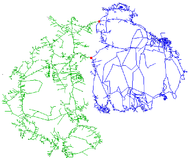
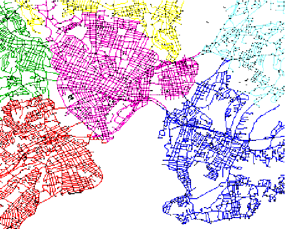
The collected data are briefly summarized in Table 4 and Table 3. To get a taste of the topic, some examples of local cell partitioning results are depicted in Fig. 2 and 1.
| Input | Partitioning | Boundary Graph | |||
|---|---|---|---|---|---|
| Road network | #Edges | #Cells | Cell sz. | #Vertices | #Edges / % size |
| USA-all | 88 742 994 | 15 862 | 5 594 | 253 641 | 524 872 / 0.59% |
| USA-east | 24 130 457 | 4 538 | 5 317 | 62 692 | 107 986 / 0.45% |
| USA-west | 12 277 232 | 2 205 | 5 567 | 23 449 | 42 204 / 0.34% |
| Texas | 7 270 602 | 1 346 | 5 366 | 17 632 | 36 086 / 0.50% |
| California | 5 503 968 | 1 011 | 5 444 | 11 408 | 16 978 / 0.31% |
| Florida | 3 557 336 | 662 | 5 373 | 5 599 | 25 898 / 0.73% |
| Road network | #Vertices | #Edges | #Cells | Avg. cell size | Time |
|---|---|---|---|---|---|
| Alabama | 811 434 | 1 926 052 | 338 | 5 698 | 11 min |
| Indiana | 800 295 | 1 975 898 | 372 | 5 311 | 16 min |
| Michigan | 860 421 | 2 145 960 | 399 | 5 378 | 61 min |
| Minnesota | 908 292 | 2 166 138 | 383 | 5 666 | 18 min |
| Arizona | 893 163 | 2 184 866 | 420 | 5 202 | 25 min |
| Georgia | 945 212 | 2 226 392 | 400 | 5 655 | 14 min |
| New York | 890 684 | 2 236 530 | 422 | 5 299 | 47 min |
| North Carolina | 1 104 258 | 2 497 764 | 409 | 6 107 | 12 min |
| Oklahoma | 1 049 680 | 2 508 862 | 436 | 5 754 | 23 min |
| Ohio | 1 085 287 | 2 761 920 | 483 | 5 404 | 38 min |
| Illinois | 1 085 287 | 2 761 920 | 530 | 5 211 | 21 min |
| Missouri | 1 291 751 | 3 020 152 | 519 | 5 891 | 34 min |
| Pennsylvania | 1 263 737 | 3 081 096 | 574 | 5 367 | 26 min |
| Virginia | 1 489 661 | 3 333 864 | 479 | 6 960 | 20 min |
| Florida | 1 387 005 | 3 488 194 | 655 | 5 325 | 30 min |
| California | 2 178 025 | 5 394 762 | 1 010 | 5 341 | 86 min |
| Texas | 2 884 762 | 7 194 984 | 1 336 | 5 385 | 135 min |
5 The Route Planning Algorithm – Queries
Having already computed the boundary graph and -reach in the preprocessing phase, we now describe a natural simplified two-stage query algorithm based on the former. In its cellular stage, as outlined in the introduction, the algorithm runs -Dijkstra’s search until all its branches get saturated at cell boundaries (typically, only one or two adjacent cells are searched). Then, in the boundary stage, virtually any established route planning algorithm may be used to finish the search (cf. Prop. 1) since is a relatively small graph (Table 3) and is free from scope consideration. E.g., we use the standard reach-based A∗ [12].
- Two-stage Query Algorithm (simplified).
-
Let a road network , a proper scope mapping , an -reach on , and the boundary graph associated with an edge partition of , be given. Assume start and target positions ; then the following algorithm computes, from to , an optimal -admissible and saturated walk in for the scope .
- 1.
Opening cellular stage. Let initially be the subgraph formed by the cell (or a union of such) containing the start . Let denote the actual boundary of , i.e. those vertices incident both with edges of and of the complement (not the same as the union of cell boundaries).
- (a)
Run -reach -Dijkstra’s algorithm (unidir.) on starting from .
- (b)
An analogical procedure is run concurrently in the reverse network on the target and . If it happens that intersect and a termination condition of bidirectional Dijkstra is met, then the algorithm stops here.
- (a)
- 2.
Boundary stage. Let be the graph created from by adding the edges from to each vertex of and from each one of to . The weights of these new edges equal the distance estimates computed in (1). (Notice that many of the weights are actually —can be ignored—since the vertices are inaccessible, e.g., due to scope admissibility or -reach.)
Run the standard reach-based A∗ algorithm on the weighted graph (while the reach refers back to ), to find an optimal path from to .
- 3.
Closing cellular stage. The path computed in (2) is easily “unrolled” into an optimal -admissible saturated walk from to in the network .
A simplification in the above algorithm lies in neglecting possible non-saturated walks between (cf. Theorem 3.4), which may not be found by an -reach-based search in (1). This happens only if are very close in a local neighborhood wrt. .
We provide here a formal description of our query algorithm in pseudocode, see Algorithm 5.1. One minor aspect of this algorithm dealing with possible “unsaturated” optimal walks in short-distance queries which cannot be properly handled by -reach-based search, is closely described next.
We also briefly comment on the use of Dijkstra’s and A* algorithms in the routing query Algorithm 5.1: While A* is obviously much better in general situations, and it is used in the boundary stage, the cellular stage is genuinly different in the fact that the search has to get to an -saturated state in all directions, and so A* would be of no help in the cellular stage (the speed-up there is achieved by different means).
One more term related to Definition 9 of graph partitioning and cells is needed in the algorithm pseudocode: For let be the set of all indices such that .
Query
Unsaturated Local Search.
Relating to line 1 of Algorithm 5.1, we now explain the necessity of running a separate local search for possible non-saturated optimal – walks in the road network. As noted in the main paper, it is an inevitable limitation of the -reach -Dijkstra’s algorithm that it may not search/discover an – walk that is optimal but not saturated (cf. Theorem 3.4). Note that the presence of such a singular walk cannot be simply tested with a condition in the cellular stage of the algorithm, and so a separate local search must be used.
Though, thanks to Def. 5 and with well distributed scope mapping, such a singular walk may occur only if the distance between is quite short, and then even not-so-elaborate route planning algorithms may be used very efficiently. To be precise, if a bidirectional search is used, then each direction is searched only until - or -saturated vertices are reached, which is a quite small subset of the whole network. (If these two search spaces do not meet, then no unsaturated – walk exists.) Furthermore, yet another natural adaptation of the classical reach concept—an “anti--reach”, can be used to accelerate the search.
Very briefly, the anti--reach of a vertex is defined as the maximum value of over all pairs of vertices such that there exists a non-saturated optimal -admissible walk from to passing through , and are its subwalks between and between . Again, this parameter is easy to compute by brute force in the network.
5.1 Experimental evaluation.
Practical performance of the query algorithm has been evaluated by multiple simulation runs on Intel Core 2 Duo mobile processor T6570 (2.1 GHz) with 4GB RAM. Our algorithms are implemented in C and compiled with gcc-4.4.1 (with -O2). We keep track of parameters such as the number of scanned vertices and the queue size that influence the amount of working memory needed, and are good indicators of suitability of our algorithm for the mobile platforms.
The collected statistical data in Table 6—namely the total numbers of scanned vertices and the maximal queue size of the search—though, reasonably well estimate also the expected runtime and mainly low memory demands of the same algorithm on a mobile navigation device. A sample query comparison to bidirectional Dijkstra’s algorithm is then depicted in Fig. 3, and some statistical data are briefly summarized in Table 5.

| Distance | Scanned vertices | Max. queue size |
|---|---|---|
| (km) | our approach / B-Dijksta | our approach / B-Dijksta |
| 2000 - 3000 | 3 225 / 28 139 196 | 60 / 4276 |
| 1000 - 2000 | 2 854 / 14 821 472 | 57 / 2477 |
| 500 - 1000 | 2 305 / 2 147 015 | 53 / 2011 |
| 0 - 500 | 1 714 / 692 769 | 41 / 1587 |
| Query distance | Hit | Scanned vertices | Max. queue size | Query time |
|---|---|---|---|---|
| (km) | cells | cellular / boundary | cellular / boundary | (ms) |
| 3000 - | 277 | 1 392 / 3 490 | 60 / 58 | 8.2 + 29.8 |
| 2000 - 3000 | 139 | 1 411 / 1 814 | 64 / 52 | 7.9 + 26.9 |
| 1000 - 2000 | 57 | 1 343 / 1 511 | 57 / 49 | 7.7 + 22.8 |
| 500 - 1000 | 25 | 1 113 / 1 192 | 53 / 38 | 8.1 + 19.0 |
| 0 - 500 | 10 | 998 / 716 | 41 / 34 | 6.9 + 16.1 |
6 Conclusions
We have introduced a new concept of scope in the static route planning problem, aiming at a proper formalization of vague “route comfort” based on anticipated additional metadata of the road network. At the same time we have shown how the scope concept nicely interoperates with other established tools in route planning; such as with vertex-separator partitioning and with the reach concept. Moreover, our approach allows also a smooth incorporation of local route restrictions and traffic regulations modeled by so-called maneuvers [17].
On the top of formalizing desired “comfortable routes”, the proper mixture of the aforementioned classical concepts with scope brings more added values; very small size of auxiliary metadata from preprocessing (Table 3) and practically very efficient optimal routing query algorithm (Table 6). The small price to be paid for this route comfort, fast planning, and small size of auxiliary data altogether, is a marginal increase in the weight of an optimal scope admissible walk as compared to the overall optimal one (scope admissible walks form a proper subset of all walks). Simulations with the very basic scope mapping from Table 1 reveal an average increase of less than for short queries up to km, and for queries above km. With better quality road network metadata and a more realistic utility weight function (such as travel time) these would presumably be even smaller numbers.
At last we very briefly outline two directions for further research on the topic.
- i.
With finer-resolution road metadata, it could be useful to add a few more scope levels and introduce another query stage(s) “in the middle”.
- ii.
The next natural step of our research is to incorporate dynamic road network changes (such as live traffic info) into our approach—more specifically into the definition of scope-admissible walks; e.g., by locally re-allowing roads of low scope level nearby such disturbances.
References
- [1] I. Abraham, D. Delling, A. V. Goldberg, and R.F . Werneck. A hub-based labeling algorithm for shortest paths in road networks. In SEA’11, pages 230–241, 2011.
- [2] I. Abraham, A. Fiat, A. V. Goldberg, and R. F. Werneck. Highway dimension, shortest paths, and provably efficient algorithms. In SODA’10: Proceedings of the 21st Annual ACM-SIAM Symposium on Discrete Algorithms, pages 782–793, 2010.
- [3] H. Bast, S. Funke, D. Matijevic, P. Sanders, and D. Schultes. In transit to constant shortest-path queries in road networks. In ALENEX’07: Proceedings of the 9th Workshop on Algorithm Engineering and Experiments, pages 46–59, 2007.
- [4] R. Bauer and D. Delling. SHARC: Fast and robust unidirectional routing. J. Exp. Algorithmics, 14:4:2.4–4:2.29, January 2010.
- [5] E. Brunel, D. Delling, A. Gemsa, and D. Wagner. Space-efficient SHARC-routing. In SEA’10: Proceedings of the 9th International Symposium on Experimental Algorithms, pages 47–58, 2010.
- [6] B. Cherkassky, A. V. Goldberg, and T. Radzik. Shortest paths algorithms: Theory and experimental evaluation. Mathematical Programming, 73(2):129–174, 1996.
- [7] D. Delling, P. Sanders, D. Schultes, and D. Wagner. Engineering route planning algorithms. In Algorithmics of Large and Complex Networks. Lecture Notes in Computer Science, pages 117–139, Berlin, Heidelberg, 2009. Springer.
- [8] D. Delling and D. Wagner. Time-dependent route planning. In Robust and Online Large-Scale Optimization, LNCS, pages 207–230. Springer, 2009.
- [9] E. Dijkstra. A note on two problems in connexion with graphs. Numerische Mathematik, 1:269–271, 1959.
- [10] R. Geisberger, P. Sanders, D. Schultes, and D. Delling. Contraction hierarchies: Faster and simpler hierarchical routing in road networks. In Catherine McGeoch, editor, Experimental Algorithms, volume 5038 of Lecture Notes in Computer Science, pages 319–333. Springer Berlin / Heidelberg, 2008.
- [11] A. V. Goldberg and Ch. Harrelson. Computing the shortest path: A* search meets graph theory. In SODA’05: Proceedings of the 16th Annual ACM-SIAM Symposium on Discrete Algorithms, pages 156–165, 2005.
- [12] A. V. Goldberg, H. Kaplan, and R. F. Werneck. Reach for A*: Efficient point-to-point shortest path algorithms. Technical report, Microsoft Research, 2005.
- [13] A. V. Goldberg, H. Kaplan, and R. F. Werneck. Better landmarks within reach. In WEA’07: Proceedings of the 6th international conference on Experimental algorithms, pages 38–51, Berlin, Heidelberg, 2007. Springer-Verlag.
- [14] A. V. Goldberg and R. F. Werneck. Computing point-to-point shortest paths from external memory. In ALENEX/ANALCO’05: Proceedings of the 7th Workshop on Algorithm Engineering and Experiments and the 2nd Workshop on Analytic Algorithmics and Combinatorics, pages 26–40, 2005.
- [15] R. Gutman. Reach-based routing: A new approach to shortest path algorithms optimized for road networks. In ALENEX’04: Proceedings of the 6th Workshop on Algorithm Engineering and Experiments, pages 100–111, 2004.
- [16] P. E. Hart, N. J. Nilsson, and B. Raphael. A formal basis for the heuristic determination of minimum cost paths. IEEE Transactions on Systems Science and Cybernetics SSC4, 4(2):100–107, 1968.
- [17] P. Hliněný and O. Moriš. Generalized maneuvers in route planning. ArXiv e-prints, arXiv:1107.0798, July 2011.
- [18] J. Maue, P. Sanders, and D. Matijevic. Goal-directed shortest-path queries using precomputed cluster distances. J. Exp. Algorithmics, 14:3.2–3.27, 2009.
- [19] S. H. Murdock. 2009 TIGER/Line Shapefiles. Technical Documentation published by U.S. Census Bureau, 2009.
- [20] I. S. Pohl. Bi-directional and heuristic search in path problems. PhD thesis, Stanford University, Stanford, CA, USA, 1969.
- [21] P. Sanders and D. Schultes. Engineering highway hierarchies. In ESA’06: Proceedings of the 14th conference on Annual European Symposium, pages 804–816, London, UK, 2006. Springer-Verlag.
- [22] P. Sanders, D. Schultes, and Ch. Vetter. Mobile route planning. In European Symposium on Algorithms, pages 732–743, London, UK, 2008. Springer-Verlag.
- [23] D. Schultes. Route Planning in Road Networks. PhD thesis, Karlsruhe University, Karlsruhe, Germany, 2008.
- [24] D. Schultes and P. Sanders. Dynamic highway-node routing. In WEA’07: Proceedings of the 6th international conference on Experimental algorithms, pages 66–79, Berlin, Heidelberg, 2007. Springer-Verlag.