Degrees of Freedom Region for an Interference Network with General Message DemandsThanks: L. Ke was with the Department of Electrical and Computer Engineering, Iowa State University, Ames, IA 50011 USA. He is now with Qualcomm Inc., San Diego, CA 92121 (e-mail: lke@qualcomm.com).Thanks: A. Ramamoorthy (corresponding author) and Z. Wang are with the Department of Electrical and Computer Engineering, Iowa State University, Ames, IA 50011 USA (e-mail: {adityar, zhengdao}@iastate.edu).Thanks: H. Yin is with the Department of Electronics Engineering and Information Science, University of Science and Technology of China, Hefei, Anhui, 230027, P.R.China (e-mail: yhr@ustc.edu.cn). He was visiting Iowa State University when this work was performed.Thanks: The material in this work was presented in part at the 2011 IEEE International Symposium on Information Theory. This work was supported in part by NSF grant CCF-1018148.
Abstract
We consider a single hop interference network with transmitters and receivers, all having antennas. Each transmitter emits an independent message and each receiver requests an arbitrary subset of the messages. This generalizes the well-known -user -antenna interference channel, where each message is requested by a unique receiver. For our setup, we derive the degrees of freedom (DoF) region. The achievability scheme generalizes the interference alignment schemes proposed by Cadambe and Jafar. In particular, we achieve general points in the DoF region by using multiple base vectors and aligning all interferers at a given receiver to the interferer with the largest DoF. As a byproduct, we obtain the DoF region for the original interference channel. We also discuss extensions of our approach where the same region can be achieved by considering a reduced set of interference alignment constraints, thus reducing the time-expansion duration needed. The DoF region for the considered system depends only on a subset of receivers whose demands meet certain characteristics. The geometric shape of the DoF region is also discussed.
Index Terms:
Interference alignment, degrees of freedom region, multicast, multiple-input multiple-output, interference network.I Introduction
In wireless networks, receivers need to combat interference from undesired transmitters in addition to the ambient noise. Interference alignment has emerged as an important technique in the study of fundamental limits of such networks [1, 2]. Traditional efforts in dealing with interference have focused on reducing the interference power, whereas in interference alignment the focus is on reducing the dimensionality of the interference subspace. The subspaces of interference from several undesired transmitters are aligned so as to minimize the dimensionality of the total interference space. For the -user -antenna interference channel, it is shown that alignment of interference is simultaneously possible at all the receivers, allowing each user to transmit at approximately half the single-user rate in the high signal-to-noise ratio (SNR) scenario [3]. The idea of interference alignment has been successfully applied to other interference networks as well [4, 5, 6, 7, 8].
The vector interference alignment schemes of [3] are applicable to time-varying channels. Constant channels have been dealt with using the technique of real interference alignment [7, 9, 10, 11, 12]. The major difference between vector interference alignment and real interference alignment is that the former relies on the linear vector-space independence, while the latter relies on linear rational independence. Besides vector and real interference alignment schemes, it is also possible to utilize the ergodicity of the channel states in the so called ergodic interference alignment scheme [13].
A majority of systems considered so far for interference alignment involve only multiple unicast traffic, where each transmitted message is only demanded by a single receiver. However, there are wireless multicast applications where a common message may be demanded by multiple receivers, e.g., in a wireless video broadcasting. Such general message request sets have been considered in [14] where each message is assumed to be requested by an equal number of receivers. Ergodic interference alignment was employed to derive an achievable sum rate. A different but related effort is the study of the compound multiple-input single-output broadcast channel [7, 8], where the channel between the base station and the mobile user is drawn from a known discrete set. As pointed out in [7], the compound broadcast channel can be viewed as a broadcast channel with common messages, where each message is requested by a group of receivers. Therefore, its total degrees of freedom (DoF) is also the total DoF of a broadcast channel with different multicast groups. It is shown that using real interference alignment scheme, the outer bound of the compound broadcast channel [6] can be achieved regardless of the number of channel states one user can have. The compound setting was also explored for the channel and the interference channel in [7], where the total number of DoF is shown to be unchanged for these two channels. However, the DoF region was not identified in [7].
In this paper, we consider a natural generalization of the multiple unicasts scenario considered in the work of Cadambe and Jafar [3]. We consider a setup where there are transmitters and (that may be different from ) receivers, each having antennas. Each transmitter emits a unique message and each receiver is interested in an arbitrary subset of the messages. That is, we consider interference networks with general message demands. Our main result in this paper is the DoF region for such networks. One main observation is that by appropriately modifying the achievability schemes of [3, 4], we can achieve any point in the DoF region. To the best of our knowledge, the DoF region in this scenario has not been obtained before. Our main contributions can be summarized as follows
- (i)
We completely characterize the DoF region for interference networks with general message demands. We achieve any point in the DoF region by using multiple base vectors and aligning the interference at each receiver to its largest interferer. The geometric shape of the region is also discussed.
- (ii)
As a corollary, we obtain the DoF region for the case of multiple unicasts considered in [3]. We also provide an additional proof based on timesharing for this case.
- (iii)
We discuss extensions of our approach where the DoF region can be achieved by considering fewer interference alignment constraints, allowing for interference alignment over a shorter time duration. We show that the region depends only on a subset of receivers whose demands meet certain characteristics.
This paper is organized as follows. The system model is given in Section II. We present the DoF region of this system, and establish its achievability and converse in Section III. We discuss the approaches for reducing the number of alignment constraints, the DoF region for the -user -antenna interference channel of [3], the total DoF in Section IV. Finally, Section V concludes our paper.
We use the following notation: boldface uppercase (lowercase) letters denote matrices (vectors). Real, integer, and complex numbers sets are denoted by , and , respectively. We define , and define similarly. We use to denote the circularly symmetric complex Gaussian (CSCG) distribution with zero mean and unit variance. For a vector , is the th entry. For two matrices and , implies that the column space of is a subspace of the column space of .
II System Model
Consider a single hop interference network with transmitters and receivers. Each transmitter has one and only one independent message. For this reason, we do not distinguish between the indices for messages and that for transmitters. Each receiver can request an arbitrary set of messages from multiple transmitters. Let be the set of indices of those messages requested by receiver . We assume that all the transmitters and receivers have antennas. The channel between transmitter and receiver at time instant is denoted as . We assume that the elements of all the channel matrices at different time instants are independently drawn from some continuous distribution. In addition, the channel gains are bounded between a positive minimum value and a finite maximum value to avoid degenerate channel conditions. The received signal at the th receiver can be expressed as
where is an independent CSCG noise with each entry distributed, and is the transmitted signal of the th transmitter satisfying the following power constraint
Henceforth, we shall refer to the above setup as an interference network with general message demands. Our objective is to study the DoF region of an interference network with general message demands when there is perfect CSI at receivers and global CSI at transmitters. Denote the capacity region of such a system as . The corresponding DoF region is defined as
If and , the general model we considered here will reduce to the well-known user antenna interference channel as in [3].
III DoF Region of Interference Network with General Message Demands
In this section, we derive the DoF region of the interference network with general message demands. Our main result can be summarized as the following theorem.
Theorem 1
The DoF region of an interference network with general message demands with transmitters, receivers, and antennas is given by
| (1) |
where is the set of indices of messages requested by receiver , . ∎
III-A Discussion on the DoF region
III-A1 The converse argument
To show the region given by (1) is an outer bound, we use a genie argument which has been used in several previous papers, e.g., [15, 3]. In short, we assume that there is a genie who provides all the interference messages except for the interference message with the largest DoF to receiver . Thus, receiver can decode its intended messages, following which it can subtract the intended message component from the received signal so that the remaining interfering message can also be decoded. Hence, (1) follows due to the multiple access channel outer bound.

III-A2 Geometric Shape of the DoF region
The DoF region is a convex polytope, as is evident from the representation in (1). The inequalities in (1) characterize the polytope as the intersection of half spaces, each defined by one inequality. Note that all the coefficients of the DoF terms in each inequality are either zero or one. That is, all the inequalities are of the form
| (2) |
where is a subset of . This can be seen by expanding each inequality in (1) containing a “max” term into several inequalities that do not contain the maximum operator. For example, we can expand into and . In a -dimensional space, the set of points defined by and is a simplex of dimensions. For example, describe a one-dimensional simplex. This simplex, together with the lines (planes) and defines a subset of the 2-dimensional space, which is a right triangle of equal sides. When considering such an inequality in the -dimensional space, each such inequality describes a cylinder set whose projection into the -dimensions is the aforementioned subset enclosed by the simplex and the planes . See Fig. 1 for an illustration in the case of and . The whole DoF region therefore is the intersection of such cylinder sets.
It is also possible to specify convex polytopes via its vertices. Theoretically it is possible to find all the vertices of the DoF region by solving a set of linearly independent equations, by replacing a subset of inequalities to equalities, and verifying that the solution satisfies all other constraints. However the number of such equations can be as large as , where is the total number of (expanded) inequalities. Nevertheless, in some special cases as we will see later, it is possible to find the vertices exactly.
In the following part, we will use a simple example to demonstrate the DoF region and reveal the basic idea of our achievability scheme.

III-B An example of the general message demand and the DoF region
We first show the geometric picture of the DoF region for a specific example, which is useful for developing the general achievability scheme.
Consider an interference network with transmitters and receivers; see Fig. 3. All the transmitters and receivers have single antenna; that is, . Assume , and . The DoF region of the system according to Theorem 1 is as follows
The region is 4-dimensional and hence difficult to illustrate. However, if the DoF of one message, say , is fixed, the DoF region of the other messages can be illustrated in lower dimensions as a function of ; see Fig. 3.
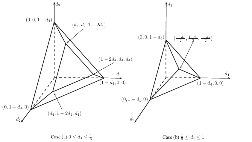
We first investigate the region when , for which the coordinates of the vertices are given in Fig. 3, case (a). The achievability of the vertices on the axes is simple as there is no need of interference alignment. Time sharing between the single-user rate vectors is sufficient. For the remaining three vertices, we only need to show the achievability of one point as the achievability of the others are essentially the same by swapping the message indices.
We will use the scheme based on [3] to do interference alignment and show is achievable for any . Let denote the duration of the time expansion in number of symbols. Here and after, we use the superscript tilde to denote the time expanded signals, e.g., , which is a size diagonal matrix (recall that ). Denote the beamforming matrix of transmitter as . First, we want messages 3 and 4 to be aligned at receivers 1. Notice that messages 3 and 4 have the same number of DoF. We choose to design beamforming matrices such that the interference from transmitter 4 is aligned to interference from transmitter 3 at receiver 1. Therefore we have the following constraint
| (7) |
Note that the interference due to transmitter 1 has a larger DoF at receiver 2; thus, we must align interference from transmitter 4 to interference from transmitter 1 at receiver 2, which leads to
| (8) |
Similarly at receiver 3, we have
| (9) |
The alignment relationship is also shown in Fig. 2. Notice that is larger than , and . Therefore it is possible to design into two parts as , where is used for transmitting part of the message 1 with the same DoF as other messages. The second part is used for transmitting the remaining DoF of message 1. In addition, all the columns in are linearly independent.
The design of can be addressed by the classic asymptotic interference alignment scheme in [3]. The beamforming matrices in [3] are chosen from a set of beamforming columns, whose elements are generated from the product of the powers of certain matrices and a vector. We term such a vector as a base vector in this paper. The base vector was chosen to be the all-one vector in [3]. The scheme proposed in [3] was further explored for wireless network [4] with multiple independent messages at single transmitter, where multiple independent and randomly generated base vectors are used for constructing the beamforming matrices. In our particular example, as no interference is aligned to the second part of message 1, we may choose an independent and randomly generated matrix for . However, in general we need to construct the beamforming matrices in a structured manner using multiple base vectors as we will see in Section III-C. The DoF point can be achieved asymptotically when the number of time expansion goes to infinity. We omit further details of beamforming construction for this particular example.
The DoF region of case (b) in Fig. 3 can be achieved similarly by showing that the vertex is achievable. This also requires the multiple base vector technique.
We remark that the DoF region in this example can also be formulated as the convex hull of the following vertices . The achievability of the whole DoF therefore can be alternatively established by showing that is achievable. This can be verified by exhaustively examining the basic feasible solutions for the polytope description in (III-B).
III-C Achievability of the DoF region with single antenna transmitters and receivers
We first consider the achievability scheme when all the transmitters and receivers have a single antenna, i.e., . It is evident that we only need to show any point in satisfying
| (10) |
is achievable, for otherwise the messages can be simply renumbered so that (10) is true.
III-C1 The set of alignment constraints
The achievability scheme is based on interference alignment over a time expanded channel. Based on (10), we impose the following relationship on the sizes of the beamforming matrices of the transmitters:
| (11) |
where denotes the number of columns of matrix . At receiver , we always align the interference messages with larger indices to the interference message with index , which is the interference message with the largest DoF, given as
Denote as following
which is the matrix corresponding to the alignment constraint
that enforces the interference from message to be aligned to the interference of message at receiver . Based on (11), for any matrix, we always have .
For convenience, we define the following set
In other words, is a set of vectors denoting all the alignment constraints. There exists a one-to-one mapping from a vector in to the corresponding matrix .
III-C2 Time expansion and base vectors
It is not difficult to see that the vertices of the DoF region given in (1) must be rational as all the coefficients and right hand side bounds are integers (either zero or one). Therefore we only need to consider the achievability of such rational vertices, although the proof below applies to any interior rational points in the DoF region as well.
For any rational DoF point within (vertex or not) satisfying (10), we can choose a positive integer , such that
| (15) |
We then use multiple base vectors to construct the beamforming matrices. The total number of base vectors is . Denote the base vectors as . Transmitter will use base vectors to construct its beamforming matrix, and the same base vectors will be used by transmitters as well (see Fig. 4). The elements of are independent and identically drawn from some continuous distribution. In addition, we assume that the absolute value of the elements of are bounded between a positive minimum value and a finite maximum value, in the same way that entries of are bounded (see Section II).

Denote , which is the total number of matrices as well. We propose to use a fold time expansion, where is a positive integer.
III-C3 Beamforming matrices design
The beamforming matrices are generated in the following manner.
- i)
Denote as the cardinality of the following set
which is the number of matrices whose exponents are within , while the other matrices can be raised to the power of . It is evident that , and .
- ii)
Transmitter uses base vectors. For base vector , it generates the following columns
where . Hence, the total number of columns of is .
- iii)
Similarly, transmitter uses base vectors. For base vector , it generates columns
(16) where
In summary, the beamforming design is as follows, for every message, we construct a beamforming column set as
The beamforming matrix is chosen to be the matrix that contains all the columns of .
III-C4 Alignment at the receivers
Assume , so that message needs to be aligned with message at receiver . We now show that this is guaranteed by our design. Let , be a base vector used by transmitter , and hence also used by transmitter . From (16), the beamforming vectors generated by at transmitter can be expressed in the following way
| (17) |
whereas those at the transmitter can be expressed as
| (18) |
Comparing the ranges of in (17) and (18), i.e., the middle terms, it can be verified that the columns in (18) multiplied with , will be a column in (17), . That is, message can be aligned to message for any such that .
The alignment scheme works due to the following reasons.
- i)
Let denote the exponent of the term for . The construction of the beamforming column set guarantees that
(19) by setting
With (19), we are guaranteed all vectors in , when left multiplied with (which has the effect of increasing the exponent of by one), generates a vector that is within the columns of . Hence the alignment is ensured.
For other terms where is not or , can be either or .
- ii)
The base vectors used by transmitter are also used by transmitter . This guarantees that if the interference from transmitter needs to be aligned with interference from transmitter , where , the alignment is ensured with the condition (19).
III-C5 Achievable Rates
It is evident that is a tall matrix of dimension . We also need to verify it has full column rank. Notice that all the entries in the upper square sub-matrix are monomials and the random variables of the monomial are different in different rows. In addition, for a given row , any two entries have different exponents. Therefore, based on [4, Lemma 1], has full column rank and
III-C6 Separation of the signal and interference spaces
Finally, we need to ensure that the interference space and signal space are linearly independent for all the receivers. Let the set of messages requested by receiver be , where . For receiver to be able to decode its desired messages, the following matrix
| (20) |
needs to have full rank for all .
Notice that for any point within
| (21) |
always holds (recall ). Therefore is a matrix that is either tall or square. For any row of its upper square sub-matrix, its elements can be expressed in the following general form:
The elements from different blocks (that is, different , ) are different due to the fact that ’s are different, hence the monomials involve different sets of random variables. Within one , two monomials are different either because they have different , or, if they have the same , the associated exponents are different. Thus matrix has the following properties.
- i)
Each term is a monomial of a set of random variables.
- ii)
The random variables associated with different rows are independent.
- iii)
No two elements in the same row have the same exponents.
It follows from [4, Lemma 1] that has full column rank with probability one.
Combining the interference alignment and the full-rank arguments, we conclude that any point satisfying (1) is achievable.
III-D Achievability of the DoF region with multiple antenna transmitters and receivers
We next present the achievability scheme for the multiple antenna case. We assume that all transmitters and receivers are equipped with the same number of antennas. An achievability scheme optimal for the total DoF has been proposed in [3] based on an antenna splitting argument. However, the same antenna splitting argument cannot be used to establish the DoF region in general because it relies on the fact that the DoF’s of the messages are equal, which is the case when the total DoF is maximized. Indeed if one attempts to perform antenna splitting with unequal DoF’s and then applies the previous scheme (Section III-C) by converting it into a single antenna instance with independent messages at each antenna, then the genie-based outer bound may rule out decoding at certain receivers.
We now show the achievability of the DoF region of multiple antenna case based on the method that was proposed in [16]. The messages are split at the transmit side and transmitted via virtual single antenna transmitters, while the receivers are still using all antennas to recover the intended messages. Therefore, the one-to-many interference alignment scheme given in [16] can be used here along with the multiple base vectors technique to achieve the DoF region.
We assume that (10) is still true. After splitting the transmitters, we now have an interference network with virtual single antenna transmitters and multiple antenna receivers. For any transmitter , the th antenna will transmit a message of DoF . In addition, the beamforming matrices for all the virtual single antenna transmitters of original system transmitter are the same, denoted as , and therefore (11) still holds. However, its size will be different from the single antenna case as we will see in the discussion below.
III-D1 The set of alignment constraints
The channels in the modified case are all in single input and multiple output representation. We denote the channel between the th antenna of transmitter and receiver as . Apparently, . The channel after time expansion is denoted as , which is a tall matrix of size . At receiver , we still align the interference messages with larger indices to the interference message with index . However, because any channel vectors from virtual single antenna transmitters to any receiver with antennas are linearly independent, it is impossible to align the interference between only two virtual single antenna transmitters. To achieve alignment at the receivers, we employ a design in [16], where the signal from one antenna is aligned with the signals coming from all the antennas of another transmitter. For our problem, we will align at receiver the message from the th antenna of transmitter with the messages from all the antennas of transmitter , for all and for all . Specifically, letting for notational simplicity, we require
| (22) |
The matrix is full rank and hence invertible. It is shown in [16] that is an matrix having block form
where all block matrices are diagonal (see Appendix A in [16]) and therefore commutable. Hence, the constraint (22) can be converted to equivalent constraints:
Similar to the single antenna case, we define a set as follows
And there exists a one-to-one mapping from a vector in to the corresponding matrix . In addition, it is easy to see that , where denotes the constraint set as defined in (III-C1) for the single antenna case.
III-D2 Time expansion and base vectors
Similar to the single antenna case, we still need to use multiple base vectors to construct the beamforming matrices. Recall is a positive integer such that (15) is still valid. The total number of base vectors is still . For transmitter , it uses base vector and all its antennas use all the base vectors. Denote . We propose to use fold time expansion.
III-D3 Beamforming matrices design
The beamforming matrices can be generated in the following way
- i)
For any given where , denote as the cardinality of the following set
Furthermore, denote as the cardinality of the following set
which is the number of matrices whose exponents are within , while the other matrices can be raised to the power of up to . It is evident that
- ii)
Transmitter uses base vectors. For base vector , it generates the following columns
where . Hence, the total number of columns of is .
- iii)
Similarly, transmitter uses base vectors. For base vector , it generates columns
(23) where
(24)
In summary, the beamforming design is as follows. For message , we construct a beamforming column set as
where satisfies (24). The beamforming matrix is chosen to be the matrix that contains all the columns of , which has columns.
III-D4 Alignment at the receivers
Notice that the beamforming columns can be divided into parts based on different values of , which determines the range of the exponents that associates with the matrices. For any fixed value of , the proof of alignment at the receivers is the same as the single antenna case.
III-D5 Achievable Rates
It is evident that is a tall matrix of dimension . We can verify that it has full column rank based on [4, Lemma 1]. Therefore, for each antenna of transmitter , the message has the following DoF
Notice that the channels are linearly independent, therefore the messages from virtual single antenna transmitters are orthogonal to each other. Hence, transmitter can send message with DoF as it has transmit antennas.
III-D6 Separation of the signal and interference spaces
Finally, we need to ensure that the interference space and signal space are linearly independent for all the receivers. This is similar to the proof in single antenna case as well. For given value of , the proof is the same. On the other hand, the blocks associated with different are apparently linear independent due to the non-overlapping range of exponents.
Hence, combining the interference alignment and the full-rank arguments, we conclude that any point satisfying (1) is achievable for multiple antenna case.
IV Discussion
In this section, we outline some alternative schemes that require a lower level of time-expansion for achieving the same DoF region, and highlight some interesting consequences of the general results developed in Section III.
IV-A Group based alignment scheme
The achievability scheme presented in Section III requires all interference messages at one receiver to be aligned with the largest one. This may introduce more alignment constraints than needed. We give an example here to illustrate this point.
Example 1
Consider a simple scenario where there are messages and 5 receivers. Without loss of generality, assuming (11) is true and , , , and . The alignment constraints associated with the first two receivers will be the following
However, in this particular case, upon inspection, one can realize that even if receiver 2 also receives message 1, the DoF region will not change. This is because the constraint at receiver 1 dictates that
However, this also implies the required constraint at receiver 2, which is
Therefore, receiver 2 can use the same alignment relationship as receiver 1, i.e., it can also decode message 1 without shrinking the DoF region. The difference between the original alignment scheme and the modified scheme of receiver 2 is illustrated in Fig. 5. ∎

The alignment scheme of Section III can be modified appropriately using the idea of partially ordered set (poset)[17].
A poset is a set and a binary relation such that for all , we have
- 1.
(reflexivity).
- 2.
and implies (transitivity).
- 3.
and implies (antisymmetry).
An element in is the greatest element if for every element , we have . An element is a maximal element if there is no element such that . If a poset has a greatest element, it must be the unique maximal element, but otherwise there can be more than one maximal element.
For two message request sets and , we say if . With this partial ordering, the collection of message request sets , with duplicate elements (message sets) removed, forms a poset. Let denote the number of maximal elements of this poset, and denote the th maximal element, . We divide the receivers into group according to the following rule: For receiver , if there exists a group index such that , then receiver is assigned to group . Otherwise, is not a maximal element, we can assign receiver to any group such that . In the case where there are multiple maximal elements of the poset that are “larger” than , we can choose the index of any of them as the group index of receiver .
With our grouping scheme, there will be at least one receiver in each group whose message request set is a superset of the message request set of any other receiver in the same group. There may be multiple such receivers in each group though. In either case, we term one such (or the one in case there is only one) receiver as the prime receiver. We choose all the receivers within one group use the same alignment relationship as the prime receiver of that group and the total number of alignment constraints is reduced. In such a way, the receivers in one group can actually decode the same messages requested by the prime receiver of that group, and they can simply discard the messages that they are not interested in.
For instance in Example 1 given in this section, we can divide 5 receivers into three groups. Receivers 1 and 2 as group 1, receivers 3 and 4 as group 2, receiver 5 as group 3 and prime receivers are 1, 3 and 5. We remark that there are multiple ways of group division as long as one receiver can only belong to one group, e.g., receiver 1 as group 1, receivers 2, 3 and 4 as group 2, receiver 5 as group 3 and prime receivers are 1, 4 and 5.
In line with the above discussion, we have the following result.
Corollary 1
The DoF region of the interference network with general message requests as in Section II is determined by the prime receivers. Adding non-prime receivers to the system will not affect the DoF region.
Proof:
This can be shown as the inequalities (1) associated with the non-prime receivers are inactive, therefore the region is dominated by the inequalities of prime receivers.
IV-B DoF region of user antenna interference channel
As we point out before, the user antenna interference channel is a special case of the model we considered in this paper, hence, its DoF region can be directly derived based on Theorem 1.
Corollary 2
The DoF region of user antenna interference channel is
| (25) |
As a special case of our interference network with general message request, the corollary requires no new proof. But we here give an alternative scheme based on simple time sharing argument.
Proof:
Without loss of generality, suppose , and , . We would like to show that is achievable.
It is obvious that
can be achieved by single user transmission. It is also known from [3] that the point
is achievable. Trivially, the point
is achievable.
By time sharing, with weights , and among the three points, in that order, it follows that the point
is achievable. This is already at least as large as the DoF we would like to have.
Remark: After the submission of our manuscript the following results have appeared that are related to our work. The DoF region for a single-antenna interference channel without time-expansion has been shown to be the convex hull of for almost all (in Lebesgue sense) channels [18]. Interestingly, this agrees with DoF region of the -user single antenna interference channel. For, it can be seen from the proof of Corollary 1 that the DoF region given in (25) can be alternatively formulated as the convex hull of the vectors . Setting will yield the desired equivalence of the two DoF regions. This equivalence, is non-trivial, however, because it shows that allowing for time-expansion, and time-diversity (channel variation), the DoF region of the interference channel is not increased — the DoF is an inherent spatial (as opposed to temporal) characteristic of the interference channel.
IV-C Length of time expansion
For the user antenna interference channel, the total length of time expansion needed in [3] is smaller than our scheme in order to achieve total DoF. This is due to the fact that when and , it is possible to choose carefully such that the cardinality of is the same as and there is one-to-one mapping between these two. For other asymmetric DoF points, it is in general not possible to choose two messages having the same cardinality of beamforming column sets. The total time expansion needed could be reduced if we use the group based alignment scheme in Section IV-A and/or design the achievable scheme for a specific network with certain DoF.
IV-D The total DoF of an interference network with general message demands
As a byproduct of our previous analysis, we can also find the total degrees of freedom for an interference network with general message demands.
Corollary 3
The total DoF of an interference network with general message demands can be obtained by a linear program shown as follows
| (26) |
∎
Corollary 4
If all prime receivers demand , , messages, and each of the messages is requested by the same number of prime receivers. Then the total DoF is
| (27) |
and is achieved by
| (28) |
Proof:
Based on Corollary 1, we only need to consider inequalities (where is the number of groups) that are associated with the prime receivers. We show that (28) achieves the maximum total DoF when all messages are requested by the same number of prime receivers. Notice that in this case we can expand the inequality of (26) into inequalities by removing the operation. Hence, we will have inequalities in total. Since each message is requested by prime receivers, for each it appears times among the inequalities for prime receivers which request , and it appears times otherwise. Summing all the inequalities we have
Hence
and the corollary is proven.
Remark 1
If messages are not requested by the same number of prime receivers it is possible to achieve a higher sum DoF than (27). We only need to show an example here. Assuming that there are transmitters and prime receivers, the message requests are . If all the transmitters send DoF, we could achieve (27). However, choosing will lead to sum DoF which is higher.
V Conclusions and Future Work
We derived the DoF region of an interference network with general message demands. The region is a convex polytope, which is the intersection of a number of cylindrical sets whose projections into lower dimensions are simple geometric shapes each enclosed by a simplex and the coordinate planes. In certain special cases, it is possible to find the vertices of the DoF region polytope explicitly. One such case is the -user -antenna interference channel with multiple unicasts, whose DoF region is a convex hull of simple points of the all zero vector, the scaled natural basis vectors, and a scaled all-one vector, which interestingly coincides with the DoF region recently obtained for Lebesgue-a.e. constant coefficient channels with no time diversity.
Our achievability scheme for deriving the DoF region operates by generating beamforming columns with multiple base vectors over time expanded channel, and aligning the interference at each receiver to its largest interferer. We also showed that the DoF region is determined by a subset of receivers (called prime receivers), that can be identified by examining the message demands of the receivers. We provided an alternate interference alignment scheme in this scenario, where the certain receivers share the same alignment relationship, which helps to reduce the required duration of for time-expansion.
It would be interesting to consider general message demands in other interference networks. For instance, if each transmitter has multiple messages, the receiver demands may result in alignment constraints that cannot be satisfied in the same manner as described in this paper. On the other hand, the usage of multiple base vectors may be useful in proving achievability for other problems where interference alignment is applicable.
References
- [1] M. Maddah-Ali, A. Motahari, and A. Khandani, “Signaling over MIMO Multi-Base Systems: Combination of Multi-Access and Broadcast Schemes,” in Proc. IEEE Intl. Symp. on Info. Theory, 2006, pp. 2104–2108.
- [2] S. Jafar and S. Shamai, “Degrees of freedom region of the MIMO channel,” IEEE Trans. Inform. Theory, vol. 54, no. 1, pp. 151–170, Jan. 2008.
- [3] V. Cadambe and S. Jafar, “Interference alignment and degrees of freedom of the user interference channel,” IEEE Trans. Inform. Theory, vol. 54, no. 8, pp. 3425–3441, Aug. 2008.
- [4] V. Cadambe and S. Jafar, “Interference Alignment and the Degrees of Freedom of Wireless Networks,” IEEE Trans. Inform. Theory, vol. 55, no. 9, pp. 3893–3908, Sept. 2009.
- [5] C. Suh and D. Tse, “Interference Alignment for Cellular Networks,” in Proc. of Allerton Conf. Commun., Control, and Computing, 2008, pp. 1037–1044.
- [6] H. Weingarten, S. Shamai, and G. Kramer, “On the compound MIMO broadcast channel,” in Proceedings of Annual Information Theory and Applications Workshop UCSD, 2007.
- [7] T. Gou, S. Jafar, and C. Wang, “On the Degrees of Freedom of Finite State Compound Wireless Networks,” IEEE Trans. Inform. Theory, vol. 57, no. 6, pp. 3286–3308, June 2011.
- [8] M. A. Maddah-Ali, “On the Degrees of Freedom of the Compound MIMO Broadcast Channels with Finite States,” 2009. [Online]. Available: http://arxiv.org/abs/0909.5006
- [9] G. Bresler, A. Parekh, and D. N. C. Tse, “The approximate capacity of the many-to-one and one-to-many gaussian interference channels,” IEEE Trans. Inform. Theory, vol. 56, no. 9, pp. 4566–4592, Sept. 2010.
- [10] S. Sridharan, A. Jafarian, S. Vishwanath, S. A. Jafar, and S. Shamai, “A layered lattice coding scheme for a class of three user gaussian interference channels,” in 46th Annual Allerton Conference Control, and Computing, on Communication, 2008, pp. 531–538.
- [11] R. H. Etkin and E. Ordentlich, “On the degrees-of-freedom of the -user gaussian interference channel,” 2009. [Online]. Available: http://arxiv.org/abs/0901.1695
- [12] A. S. Motahari, S. O. Gharan, M. A. Maddah-Ali, and A. K. Khandani, “Real interference alignment: Exploiting the potential of single antenna systems,” 2009. [Online]. Available: http://arxiv.org/abs/0908.2282
- [13] B. Nazer, S. Jafar, M. Gastpar, and S. Vishwanath, “Ergodic interference alignment,” in Proc. IEEE Intl. Symp. on Info. Theory, 2009, pp. 1769–1773.
- [14] B. Nazer, M. Gastpar, S. Jafar, and S. Vishwanath, “Interference alignment at finite SNR: General message sets,” in Proc. of Allerton Conf. Commun., Control, and Computing, 2009, pp. 843–848.
- [15] S. Jafar and M. Fakhereddin, “Degrees of freedom for the MIMO interference channel,” IEEE Trans. Inform. Theory, vol. 53, no. 7, pp. 2637–2642, July 2007.
- [16] T. Gou and S. Jafar, “Degrees of Freedom of the User MIMO Interference Channel,” IEEE Trans. Inform. Theory, vol. 56, no. 12, pp. 6040–6057, Dec. 2010.
- [17] B. A. Davey and H. A. Priestley, Introduction to lattices and order. Cambridge University Press, 2002.
- [18] Y. Wu, S. Shamai (Shitz), and S. Verdú, “Degrees of freedom of the interference channel: a general formula,” in Proc. IEEE Intl. Symp. on Info. Theory, 2011, pp. 1344–1348.