The Catanese-Ciliberto-Mendes Lopes surfaceThanks: The author is partially supported by NSF grant DMS 0905917

Catanese-Ciliberto-Mendes Lopes surface (CaCiMe or CCM surface in short) $M$ is a complex surface constructed in [CCM] (and discussed in [HP] and [P]), which is topologically a genus $2$ surface bundle over a surface of genus $2$. Recently in [AP] this surface is used in interesting smooth manifold constructions. While inspecting [AP] we felt that first this interesting complex surface $M$ deserves a careful topological study of its own. Generally, drawing handlebody pictures of circle bundles over $3$-manifolds, or $3$-manifold bundles over circles is relatively easy compare to surface bundles of surfaces (e.g.[AK] and [A1]). Here we take this opportunity to introduce a new technique to draw a surface bundle over a surface, which avoids “turning handles upside down” process. This manifold $M$ is a good test case to understand many of the general difficulties one encounters in drawing surface bundles over surfaces, as well as taking their fiber sum. We draw the handlebody picture of $M$ in such a way that all the tori used in the constructions of [AP] are clearly visible. This combined with the log transform picture (e.g. [AY]) will allow one to see the “Lutinger surgery” constructions of [AP] in a concrete geometric way.

Let $\Sigma_{g}$ denote the surface of genus $g$. Let $\tau_{2}:\Sigma_{2}\to\Sigma_{2}$ be the hyperelliptic involution and $\tau_{3}:\Sigma_{3}\to\Sigma_{3}$ be the free involution induced by $180^{o}$ rotation, as indicated in Figure 1. The CaCiMe surface $M$ is the complex surface obtained by taking the quotient of $\Sigma_{2}\times\Sigma_{3}$ by the product involution:

By projecting to the second factor we can describe $M$ as a $\Sigma_{2}$-bundle over $\Sigma_{2}=\Sigma_{3}/\tau_{3}$. Let $A$ denote the twice punctured $2$-torus $A=T^{2}-D^{2}_{-}\sqcup D^{2}_{+}$. Then clearly $M$ is obtained by identifying the two boundary components of $\Sigma_{2}\times A$ by the involution induced by $\tau_{2}$ (notice $A$ is the interior of the fundamental domain of the action $\tau_{3}$). By deforming $A$ as in Figure 2, we see that $M=E\;\natural\;E^{\prime}$ is obtained by fiber summing two $\Sigma_{2}$ bundles over $T^{2}$, where $E$ is the trivial bundle $\Sigma_{2}\times T^{2}\to T^{2}$, and

We will build a handlebody of $M$ by a step by step process drawing the following handlebodies in the given order, also we will concretely identify the indicated diffeomorphisms:

• (a)

  $E_{0}=E-\Sigma_{2}\times D^{2}=\Sigma_{2}\times(T^{2}-D^{2})$

• (b)

  $E^{\prime}_{0}=E^{\prime}-\Sigma_{2}\times D^{2}$

• (c)

  $f_{1}:\partial E_{0}\stackrel{{\scriptstyle\approx}}{{\longrightarrow}}\Sigma_{2}\times S^{1}$

• (d)

  $f_{2}:\partial E^{\prime}_{0}\stackrel{{\scriptstyle\approx}}{{\longrightarrow}}\Sigma_{2}\times S^{1}$

• (e)

  $M=-E_{0}\smile_{f_{2}^{-1}\circ f_{1}}E^{\prime}_{0}$

One way to to perform the gluing operation (e) is to turn the handlebody $E_{0}$ upside down and attach its dual handlebody to top of $E_{0}^{\prime}$, getting $M=-E_{0}\smile E_{0}^{\prime}$ (e.g. the technique used in [A1]). In this paper we choose another way which amounts to identifying the boundaries of the two handlebodies $-E_{0}$ and $E_{0}^{\prime}$ by a cylinder $\partial E_{0}\times I$

Though this seems a trivial distinction, it makes a big difference in constructing the handlebodies. One advantage of this technique is that we see the imbedded tori used in the construction of [AP] clearly.

Figure 3 (a disk with two pairs of $1$-handles and a $2$-handle, where only the attaching arcs of the $1$-handles are drawn) describes a handlebody for $\Sigma_{2}$, and Figure 4 is $\Sigma_{2}\times[0,1]$. Hence Figure 5 is a handlebody of $\Sigma_{2}\times S^{1}$ (compare [AK]). Figure 6 is the same as Figure 5, except it is drawn as a Heegard diagram. So Figure 7 describes a handlebody picture of of $\Sigma_{2}\times S^{1}\times S^{1}=\Sigma_{2}\times T^{2}$. A close inspection shows that removing the $2$-handle, denoted by $c$, from Figure 7 gives the handlebody of $E_{0}$ ($c$ is the disk boundary in $T^{2}-D^{2}$, as the attaching circle of the $2$-handle corresponding to $D^{2}$; more precisely it is the upside down $2$-handle of the missing $\Sigma_{2}\times D^{2}$ which is removed from $E_{0}$).

Next in Figures 8 through 11 we gradually convert the “pair of balls” notation of the $1$-handles of Figure 7 to the “circle-with-dot” notation of [A2] (i.e. carving). Figure 11 is the same as Figure 7, except that all of its $1$-handles are drawn in circle-with-dot notation. For the benefit of the reader we did this transition in several steps: First in Figure 8 we converted a pair of $1$-handles of Figure 7 to the circle-with-dot notation, then in Figure 11 converted the remaining $1$-handles. Figure 9 shows how to perform local isotopies near the attaching balls of $1$-handles to go to intermediate picture Figure 10 were the attaching balls are drawn as flat arcs. We then converted the flat arcs to the circle-with dots. In Figure 11 all the 2-handles are attached with $0$-framing.

Next we construct a difeomorphism $f_{1}:\partial E_{0}\stackrel{{\scriptstyle\approx}}{{\longrightarrow}}\Sigma_{2}\times S^{1}$. First by an isotopy we go from Figure 11 to Figure 12, then by replacing the circles with dots with 0-framed circles, and by performing the handle slides to Figure 12 as indicated by the arrows, we obtain the first picture of Figure 13, and by further handle slides and cancellations we obtain the second picture of Figure 13, which is $\Sigma_{2}\times D^{2}$. In the Figure 13 we also indicate where this diffeomorphism throws the linking loops $a_{1},b_{1},a_{2},b_{2},c$. Finally in Figure 14 we describe the diffeomprphism we constructed $f_{1}:\partial E_{0}\to\Sigma_{2}\times S^{1}$ in a much more concrete way by indicating the images of the arcs shown in the figure. Though going from Figure 11 to Figure 14 is locally a routine process, finding the correct handle sliding moves and locating and keeping the track of those arcs is the most time consuming part of this work.

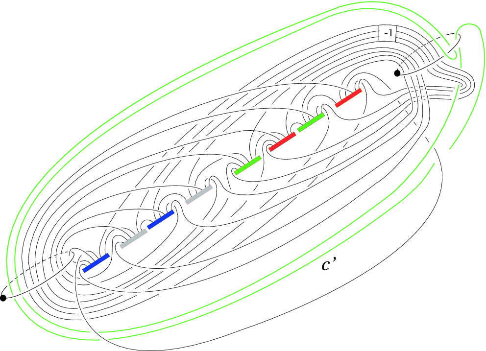
Figures 15 and 16 shows that the diffoemorphism $\tau_{2}:\Sigma_{2}\to\Sigma_{2}$ is induced from $180^{0}$ rotation of the disk with four $1$-handles. Having noted this, we proceed exactly as Figure 7 through Figure 11, except that we replace Figure 7 by Figure 17 (due to twisting by $\tau_{2}:\Sigma_{2}\to\Sigma_{2}$). So Figure 20 is the handlebody of $E_{0}^{\prime}$ (without the curve denoted by $c^{\prime}$), and Figure 22 describes a diffeomorphism $f_{2}:\partial E_{0}^{\prime}\to\Sigma_{2}\times S^{1}$

To construct $M=-E_{0}\smile E_{0}^{\prime}$ we draw the handlebodies $-E_{0}$ and $E_{0}^{\prime}$ side by side, and glue their boundaries to the two boundary components of the cylinder $\Sigma_{2}\times S^{1}\times I$. This gluing is done by identfying $1$-handle circles $\{a_{1},b_{1},a_{2},b_{2},c\}$ (Figure 13) of $\partial E_{0}\approx\Sigma_{2}\times S^{1}$ and of $\partial E_{0}^{\prime}\approx\Sigma_{2}\times S^{1}$ by 2-handles. Now Figure 14 and Figure 22 gives us exactly the information needed to draw the CaCiMe surface $M=-E_{0}\smile_{f_{2}^{-1}\circ f_{1}}E_{0}^{\prime}$ as shown in Figure 23 (all the circles are $0$-framed $2$-handles).

Cacime surface has its own place in the classification scheme of complex surfaces, as stated in the following theorem:

Recall $b_{1}(X)=2q(X)$, $K_{X}=c_{1}(X)$ and $3\sigma(X)=c_{1}^{2}(X)-2\chi(X)$, Noether formula: $1-q(X)+p_{g}(X)=\frac{1}{12}[\;c_{1}^{2}(X)+c_{2}(X)\;]$ $\Rightarrow$ So if (b) holds $b_{2}(X)=14$ ad $\sigma(X)=0$ So the Cacime surface $X$ is homology equivalent to $\#7(S^{2}\times S^{2})\#6(S^{1}\times S^{3})$, and its fundamental group presumably can be calculated from its fibration structure provided its monodromies are determined, But now we can easily calculate the fundamental group as well as the other topological invariants from its handlebody picture in Figure 23.

References

- [A1] S. Akbulut, Cappell-Shaneson’s s-cobordism , GT vol.6, (2002) 425-494.
- [A2] S. Akbulut, On -dimensional homology classes of -manifolds, Math. Proc. Camb. Phil. Soc. 82 (1977), 99-106.
- [A3] S. Akbulut, Nash homotopy spheres are standard, Proc.GGT (2010) 135-144, arXiv:1102.2683
- [A4] S. Akbulut, The Akhmedov-Park exotic , arXiv:1106.3924
- [A5] S. Akbulut, The Akhmedov-Park exotic . arXiv:1107.3073
- [AK] S. Akbulut and R. Kirby , An exotic involution of , Topology, vol.18, (1979), 75-81
- [CCM] F. Catanese, C. Ciliberto, M. Mendes Lopes, On the classification of irregular surfaces of general type with non birational bicanonical map, Trans. Amer. Math. Soc. 350 (1998), 275-308.
- [AP] A. Akhmedov and B.D.Park, Exotic Smooth Structures on , arXiv:1005.3346v4.
- [AY] S. Akbulut and K. Yasui, Corks, Plugs and exotic structures, Journal of Gökova Geometry Topology, volume 2 (2008), 40–82.
- [HP] C. D. Hacon and R. Pardini, Surfaces wih , Trans. Amer. Math. Soc. 354 (2002), 2631-2638.
- [P] G.P. Pirola, Surfaces with , Manuscripta Math. 108, no. 2 (2002), 163-170.