\PTPindex

Quark-Model Baryon-Baryon Interaction Applied to the Neutron-Deuteron Scattering (II)

Polalization Observables of the Elastic Scattering

Kenji Fukukawa and Yoshikazu Fujiwara

Abstract

The neutron-deuteron ( $nd$ ) scattering is solved in the Faddeev formalism, employing the energy-independent version of the quark-model baryon-baryon interaction fss2. The differential cross sections and the spin polarization of the elastic scattering up to the neutron incident energy $E_{n}=65$ MeV are well reproduced without reinforcing fss2 with the three-body force. The vector analyzing-power of the neutron, $A_{y}(\theta)$ , in the energy region $E_{n}\leq 25$ MeV is largely improved in comparison with the predictions by the meson-exchange potentials, thus yielding a partial solution of the long-standing $A_{y}$ -puzzle owing to the nonlocality of the short-range repulsion produced by the quark-model baryon-baryon interaction. The large Coulomb effect in the vector and tensor analyzing-powers in $E_{n}\leq 10$ MeV is also analyzed based on the Vincent and Phatak method and recent detailed studies by other authors.

1 Introduction

The QCD-inspired spin-flavor $SU_{6}$ quark model (QM) for the baryon-baryon interaction, developed by the Kyoto-Niigata group, has achieved accurate description of available nucleon-nucleon ( $NN$ ) data, comparable with the modern meson-exchange potentials.[1] The naive three-quark structure of the nucleon is incorporated in the microscopic framework of the resonating-group method (RGM) for two three-quark clusters, leading to the well-defined nonlocality and the energy dependence of the $NN$ interaction, inherent to the RGM framework. In particular, the short-range repulsion of the $NN$ interaction is mainly described by the quark-exchange kernel originating from the color-magnetic term of the quark-quark interaction. The energy dependence of the interaction is eliminated by the standard off-shell transformation, utilizing a square root of the normalization kernel.[2] This procedure yields an extra source of nonlocality, whose effect was examined in detail for the three-nucleon ( $3N$ ) bound state and for the hypertriton.[3] The QM baryon-baryon interaction thus constructed is expected to give quite different off-shell properties from the standard meson-exchange potentials. It is therefore interesting to examine predictions by the QM $NN$ interaction to the $3N$ scattering, especially in this renormalized framework with no explicit energy dependence.

In a previous paper,[4] referred to as I hereafter, we have developed a new algorithm to solve the Alt-Grassberger-Sandhas (AGS) equations [5] with the deuteron singularity, employing the Noyes-Kowalski method.[6, 7] Another notorious moving singularity of the free three-body Green function is treated by the standard spline interpolation technique developed by the Bochum-Krakow group.[8, 9, 10, 11] The AGS equation is solved in the momentum representation, using the off-shell RGM $t$ -matrix obtained from the energy-independent renormalized RGM kernel. The total cross sections derived from the optical theorem and $nd$ elastic differential cross sections are well reproduced up to the neutron incident energy $E_{n}=65$ MeV in the laboratory system. It was found that the predicted elastic differential cross sections have larger diffraction minima than the experiment in the energy region $E_{n}=35\,\hbox{-}\,65$ MeV, in contrast with the predictions by the meson-exchange potentials. This is in consistent with the fact that fss2 reproduces nearly correct triton binding energy without the three-body force. In these calculations, we have used the Gaussian nonlocal potential constructed from the original fss2 interaction.[12] This potential preserves not only the on-shell properties of the $t$ -matrix with the accuracy of less than 0.1 degree for the phase shift parameters, but also the nonlocality of the interaction completely, which was confirmed by recalculating the triton binding energy with this potential.[13] The calculation of the $S$ -wave $nd$ scattering length by this potential yields almost correct values $\hbox{}^{2}a_{nd}=0.66~\hbox{fm}$ for the spin doublet scattering length and $\hbox{}^{4}a_{nd}=6.30~\hbox{fm}$ for the quartet scattering length, without the three-body force and the charge dependence of the $NN$ force.[13]

In this paper, we extend the study of the $nd$ elastic scattering in I and Ref. \citenscl10 to various types of spin polarization observables, and compare them with the experimental data and predictions by other theoretical calculations. In the low-energy $nd$ and $pd$ scattering, there is a long-standing nucleon analyzing-power puzzle, which implies the failure of rigorous $3N$ calculations to account for the magnitude of the measured analyzing-power $A_{y}(\theta)$ .[14, 15, 16, 17] We find that there is no serious discrepancy in $A_{y}(\theta)$ at the low energies $E_{n}\leq 25$ MeV, although the difference of about $15\%$ still remains for the magnitude of maximum peaks. We have analyzed the low-energy $nd$ and $pd$ eigenphase shifts below the deuteron breakup threshold and found that the main origin of this improvement is the more attractive feature of the $\hbox{}^{2}S_{1/2}$ phase shift in our model, originating from the nonlocal description of the short-range repulsion.[13] The comparison of tensor-type deuteron analyzing-powers with experiment is blurred with the Coulomb effect, since all the experimental data are for the $pd$ or $dp$ scattering. We here apply the Vincent and Phatak method[18, 19] using the cut-off Coulomb potential to the $pd$ scattering, and show some preliminary results in comparison with recent detailed studies by other authors in the $E_{p}\leq 10$ MeV region.[20, 21, 22, 23, 24, 25, 26] We find that this method works well to reproduce the characteristic behavior of the forward angular distributions for the $dp$ tensor analyzing-powers.

The organization of this paper is as follows. In $\lx@sectionsign\,2.1$ , we first develop a general framework to calculate the spin polarization observables for the $nd$ elastic scattering, using the Blatt and Biedenharn technique.[27] The applications to the analyzing-power and polarization of the nucleon and deuteron, the polarization transfer for the nucleon, the nucleon to deuteron polarization transfer, and the spin correlation coefficients are made in subsections 2.2, 2.3, 2.4, and 2.5, respectively. The definition of the deuteron spin operators, used in this paper, are summarized in Appendix A, together with the relationship between various different notations. The results of polarization observables are shown in $\lx@sectionsign\,3$ . In $\lx@sectionsign\,3.1$ , we discuss the nucleon analyzing-power, focusing on the analyzing-power puzzle. The vector and tensor analyzing-powers of the deuteron are discussed in $\lx@sectionsign 3.2$ , where the Coulomb effect is important at $E_{p}\leq 10$ MeV. In $\lx@sectionsign\,3.3$ , we extend the analysis of the low-energy observables below the deuteron breakup threshold, developed in Ref. \citenscl10, by employing the present approach to the Coulomb force. Various types of polarization transfer and spin correlation coefficients are discussed in $\lx@sectionsign\,3.4$ and $\lx@sectionsign\,3.5$ , respectively. The last section is devoted to a summary.

2 Formulation

2.1 General framework

In this subsection, we derive general formulas for the spin polarization observables for the $nd$ elastic scattering by using the Blatt and Biedenharn technique.[27] This method is used in the previous paper I to calculate the differential cross sections and the extension to the various spin observables is rather straightforward. We calculate $I=Tr\,\{f{\cal S}_{i}f^{\dagger}{\cal S}_{f}\}$ , where $f$ is the $nd$ scattering amplitude defined by the partial-wave amplitudes $f^{J}_{(\ell^{\prime}S^{\prime}_{c}),(\ell S_{c})}$ in Eq. I(2.92)¹¹ 1 In the following, we cite equations of the previous paper I with adding I in front of the equation number. as

	$\displaystyle f(\widehat{{\hbox{\boldmath$q$}}}_{f},\widehat{{\hbox{\boldmath$q$}}}_{i})=4\pi\sum_{(\ell^{\prime}S^{\prime}_{c})(\ell S_{c})J}f^{J}_{(\ell^{\prime}S^{\prime}_{c}),(\ell S_{c})}\sum_{J_{z}}{\cal Y}_{(\ell^{\prime}S^{\prime}_{c})JJ_{z}}(\widehat{{\hbox{\boldmath$q$}}}_{f};{\rm spin})~{\cal Y}^{\ *}_{(\ell S_{c})JJ_{z}}(\widehat{{\hbox{\boldmath$q$}}}_{i};{\rm spin})\ ,$
			(1)

where ${\cal Y}_{(\ell S_{c})JJ_{z}}(\widehat{{\hbox{\boldmath$q$}}};{\rm spin})=\left[Y_{\ell}(\widehat{{\hbox{\boldmath$q$}}})\chi_{S_{c}}(12;3)\right]_{JJ_{z}}$ is the angular-spin wave function. The spin wave function is defined by $\chi_{S_{c}S_{cz}}(12;3)=[\chi_{1}(12)\chi_{{\scriptstyle\frac{1}{2}}}(3)]_{S_{c}S_{cz}}$ . The spin operators ${\cal S}_{i}$ and ${\cal S}_{f}$ are in general expressed as a tensor operator defined by

\displaystyle{\cal S}^{(f)}_{f_{z}}=\left[\sigma^{(s)}S^{(\lambda)}\right]^{(f)}_{f_{z}}\ ,

(2)

where $s=0$ or 1 and $\lambda=0$ , 1, or 2. The neutron spin operators $\{1,{\hbox{\boldmath$\sigma$}}\}$ and the deuteron spin operators $\{1,{\hbox{\boldmath$S$}},S^{(2)}\}$ form $4\times 9=36$ independent matrix components in the spin space spanned by $\chi_{S_{c}S_{cz}}(12;3)$ with $S_{c}=1/2$ and 3/2. The deuteron spin operators $S$ and $S^{(2)}$ are summarized in Appendix A, together with the relationship between various notations. The standard expression for the $nd$ scattering is in the Cartesian representation such as $\sigma_{\alpha}S_{\beta\gamma}$ , which are expressed by the linear combination of the tensor coupled form in Eq. (2). To calculate $I=Tr\,\{f{\cal S}_{i}f^{\dagger}{\cal S}_{f}\}$ , we use Eq. (1) and take the trace for the spin variables. Then, we obtain

$\displaystyle I$	$\displaystyle=$	$\displaystyle Tr\,\{f{\cal S}_{i}f^{\dagger}{\cal S}_{f}\}$	(3)
	$\displaystyle=$	$\displaystyle(4\pi)^{2}\sum_{(\ell^{\prime}S^{\prime}_{c})(\ell S_{c})J}\sum_{(\widetilde{\ell}^{\prime}\widetilde{S}^{\prime}_{c})(\widetilde{\ell}\widetilde{S}_{c})\widetilde{J}}f^{J}_{(\ell^{\prime}S^{\prime}_{c})(\ell S_{c})}\left\{f^{\widetilde{J}}_{(\widetilde{\ell}^{\prime}\widetilde{S}^{\prime}_{c})(\widetilde{\ell}\widetilde{S}_{c})}\right\}^{*}$
		$\displaystyle\times\sum_{J_{z}\widetilde{J}_{z}}\langle{\cal Y}_{(\ell S_{c})JJ_{z}}(\widehat{{\hbox{\boldmath$q$}}}_{i};{\rm spin})\|{\cal S}_{i}\|{\cal Y}_{(\widetilde{\ell}\widetilde{S}_{c})\widetilde{J}\widetilde{J}_{z}}(\widehat{{\hbox{\boldmath$q$}}}_{i};{\rm spin})\rangle_{\rm spin}$
		$\displaystyle\times\langle{\cal Y}_{(\widetilde{\ell}^{\prime}\widetilde{S}^{\prime}_{c})\widetilde{J}\widetilde{J}_{z}}(\widehat{{\hbox{\boldmath$q$}}}_{f};{\rm spin})\|{\cal S}_{f}\|{\cal Y}_{(\ell^{\prime}S^{\prime}_{c})JJ_{z}}(\widehat{{\hbox{\boldmath$q$}}}_{f};{\rm spin})\rangle_{\rm spin}\ ,$

where the last two matrix elements are taken only for the spin variables. We assume that the spin operators ${\cal S}_{i}$ and ${\cal S}_{f}$ are tensor operators in Eq. (2) and calculate

\displaystyle I(\lambda_{i}\mu_{i};\lambda_{f}\mu_{f})=Tr\,\{f{\cal S}^{(\lambda_{i})}_{\mu_{i}}f^{\dagger}{\cal S}^{(\lambda_{f})}_{\mu_{f}}\}\ .

(4)

We first calculate

\displaystyle J_{\lambda\mu}(\widehat{{\hbox{\boldmath$q$}}}_{i})=\langle{\cal Y}_{(\ell S_{c})JJ_{z}}(\widehat{{\hbox{\boldmath$q$}}}_{i};{\rm spin})|{\cal S}^{(\lambda)}_{\mu}|{\cal Y}_{(\widetilde{\ell}\widetilde{S}_{c})\widetilde{J}\widetilde{J}_{z}}(\widehat{{\hbox{\boldmath$q$}}}_{i};{\rm spin})\rangle_{\rm spin}\ ,

(5)

in the standard recoupling technique. It is rather easy to derive

	$\displaystyle J_{\lambda\mu}(\widehat{{\hbox{\boldmath$q$}}}_{i})$	$\displaystyle=$	$\displaystyle\frac{1}{\sqrt{4\pi}}\sum_{LM}(-)^{J-S_{c}-L}\frac{1}{\widehat{J}}~Y^{*}_{LM}(\widehat{{\hbox{\boldmath$q$}}}_{i})\sum_{\kappa\nu}\langle LM\lambda\mu\|\kappa\nu\rangle~\langle\widetilde{J}\widetilde{J}_{z}\kappa\nu\|JJ_{z}\rangle$		(6)
			$\displaystyle\times Z^{(\lambda)}_{\kappa}(\ell J\widetilde{\ell}\widetilde{J};S_{c}\widetilde{S}_{c}L)\ ,$		(6)

where the recoupling coefficient $Z^{(\lambda)}_{\kappa}(\ell J\widetilde{\ell}\widetilde{J};S_{c}\widetilde{S}_{c}L)$ is defined by

	$\displaystyle Z^{(\lambda)}_{\kappa}(\ell J\widetilde{\ell}\widetilde{J};S_{c}\widetilde{S}_{c}L)=(-)^{\ell+J-S_{c}}\,\widehat{\widetilde{\ell}}\,\widehat{J}~\langle\ell 0\widetilde{\ell}0\|L0\rangle\left[\begin{array}[]{ccc}\widetilde{\ell}&\widetilde{S}_{c}&\widetilde{J}\\[5.69054pt] L&\lambda&\kappa\\[5.69054pt] \ell&S_{c}&J\\ \end{array}\right]\langle\chi_{S_{c}}\|\|{\cal S}^{(\lambda)}\|\|\chi_{\widetilde{S}_{c}}\rangle_{\rm unc}\ ,$
			(11)

using the unitary form of the 9- $j$ coefficient and the unconventional reduced matrix element $\langle\chi_{S_{c}}||{\cal S}^{(\lambda)}||\chi_{\widetilde{S}_{c}}\rangle_{\rm unc}$ . We can use this formula both for ${\cal S}^{(\lambda_{i})}_{\mu_{i}}$ and ${\cal S}^{(\lambda_{f})}_{\mu_{f}}$ in Eq. (3), changing $\widehat{{\hbox{\boldmath$q$}}}_{i}$ to $\widehat{{\hbox{\boldmath$q$}}}_{f}$ etc. Then the sum over $J_{z}$ and $\widetilde{J}_{z}$ can be taken. We further use the symmetry property of $Z^{(\lambda)}_{\kappa}(\ell J\widetilde{\ell}\widetilde{J};S_{c}\widetilde{S}_{c}L)$ in Eq. (11):

\displaystyle Z^{(\lambda)}_{\kappa}(\widetilde{\ell}\widetilde{J}\ell J;\widetilde{S}_{c}S_{c}L)=(-)^{\lambda+\kappa+L+\widetilde{S}_{c}-S_{c}}\,Z^{(\lambda)}_{\kappa}(\ell J\widetilde{\ell}\widetilde{J};S_{c}\widetilde{S}_{c}L)\ ,

(12)

by assuming ${{\cal S}^{(\lambda)}_{\mu}}^{\dagger}=(-)^{\mu}{\cal S}^{(\lambda)}_{-\mu}$ . After all, we obtain for Eq. (4)

	$\displaystyle I(\lambda_{i}\mu_{i};\lambda_{f}\mu_{f})=\sum_{(\ell^{\prime}S^{\prime}_{c})(\ell S_{c})J}\sum_{(\widetilde{\ell}^{\prime}\widetilde{S}^{\prime}_{c})(\widetilde{\ell}\widetilde{S}_{c})\widetilde{J}}(-)^{S^{\prime}_{c}-S_{c}}~f^{J}_{(\ell^{\prime}S^{\prime}_{c})(\ell S_{c})}\left\{f^{\widetilde{J}}_{(\widetilde{\ell}^{\prime}\widetilde{S}^{\prime}_{c})(\widetilde{\ell}\widetilde{S}_{c})}\right\}^{*}$
	$\displaystyle\times\sum_{LM,L^{\prime}M^{\prime}}(-)^{\mu_{f}+L+L^{\prime}}~Y^{*}_{LM}(\widehat{{\hbox{\boldmath$q$}}}_{i})~Y_{L^{\prime}M^{\prime}}(\widehat{{\hbox{\boldmath$q$}}}_{f})\sum_{\kappa\nu}\frac{4\pi}{(\widehat{\kappa})^{2}}~\langle LM\lambda_{i}\mu_{i}\|\kappa\nu\rangle~\langle L^{\prime}M^{\prime}\lambda_{f}-\mu_{f}\|\kappa\nu\rangle$
	$\displaystyle\times Z^{(\lambda_{i})}_{\kappa}(\ell J\widetilde{\ell}\widetilde{J};S_{c}\widetilde{S}_{c}L)~Z^{(\lambda_{f})}_{\kappa}(\ell^{\prime}J\widetilde{\ell}^{\prime}\widetilde{J};S^{\prime}_{c}\widetilde{S}^{\prime}_{c}L^{\prime})\ .$		(13)

We write this expression as

	$\displaystyle I(\lambda_{i}\mu_{i};\lambda_{f}\mu_{f})=\sum_{(\ell^{\prime}S^{\prime}_{c})(\ell S_{c})J}\sum_{(\widetilde{\ell}^{\prime}\widetilde{S}^{\prime}_{c})(\widetilde{\ell}\widetilde{S}_{c})\widetilde{J}}(-)^{S^{\prime}_{c}-S_{c}}~f^{J}_{(\ell^{\prime}S^{\prime}_{c})(\ell S_{c})}\left\{f^{\widetilde{J}}_{(\widetilde{\ell}^{\prime}\widetilde{S}^{\prime}_{c})(\widetilde{\ell}\widetilde{S}_{c})}\right\}^{*}$
	$\displaystyle\times\sum_{L,L^{\prime},\kappa}C^{L,L^{\prime}}_{\kappa}(\lambda_{i}\mu_{i},\lambda_{f}\mu_{f};\widehat{{\hbox{\boldmath$q$}}}_{f},\widehat{{\hbox{\boldmath$q$}}}_{i})~Z^{(\lambda_{i})}_{\kappa}(\ell J\widetilde{\ell}\widetilde{J};S_{c}\widetilde{S}_{c}L)~Z^{(\lambda_{f})}_{\kappa}(\ell^{\prime}J\widetilde{\ell}^{\prime}\widetilde{J};S^{\prime}_{c}\widetilde{S}^{\prime}_{c}L^{\prime})\ .$		(14)

The spatial part $C^{L,L^{\prime}}_{\kappa}(\lambda_{i}\mu_{i},\lambda_{f}\mu_{f};\widehat{{\hbox{\boldmath$q$}}}_{f},\widehat{{\hbox{\boldmath$q$}}}_{i})$ can be written in various forms:

	$\displaystyle C^{L,L^{\prime}}_{\kappa}(\lambda_{i}\mu_{i},\lambda_{f}\mu_{f};\widehat{{\hbox{\boldmath$q$}}}_{f},\widehat{{\hbox{\boldmath$q$}}}_{i})$
	$\displaystyle=\sum_{MM^{\prime}\nu}(-)^{\mu_{i}}\,\frac{4\pi}{\widehat{L}\,\widehat{L}^{\prime}}\langle\kappa\nu\lambda_{i}-\mu_{i}\|LM\rangle\langle\kappa\nu\lambda_{f}\mu_{f}\|L^{\prime}M^{\prime}\rangle~Y_{L^{\prime}M^{\prime}}(\widehat{{\hbox{\boldmath$q$}}}_{f})Y^{*}_{LM}(\widehat{{\hbox{\boldmath$q$}}}_{i})$
	$\displaystyle=(-)^{\lambda_{i}+\lambda_{f}+L+L^{\prime}-\kappa}\,4\pi\sum_{ff_{z}}\langle\lambda_{i}\mu_{i}\lambda_{f}\mu_{f}\|ff_{z}\rangle\left\{\begin{array}[]{ccc}L&\lambda_{i}&\kappa\\ \lambda_{f}&L^{\prime}&f\\ \end{array}\right\}~Y_{(L^{\prime}L)ff_{z}}(\widehat{{\hbox{\boldmath$q$}}}_{f},\widehat{{\hbox{\boldmath$q$}}}_{i}),$

but the separation into the invariant part and the non-invariant part is not easy except for the $f=0$ and 1 cases. We should note that the $L$ and $L^{\prime}$ sum in Eq. (14) is only for $|L-L^{\prime}|=$ even because of the parity conservation. We use a simplified notation $C^{L,L^{\prime}}_{\kappa}(\lambda_{i}\mu_{i},\lambda_{f}\mu_{f})=C^{L,L^{\prime}}_{\kappa}(\lambda_{i}\mu_{i},\lambda_{f}\mu_{f};\widehat{{\hbox{\boldmath$q$}}}_{f},\widehat{{\hbox{\boldmath$q$}}}_{i})$ in the following and choose a special coordinate system with $\widehat{{\hbox{\boldmath$q$}}}_{f}=(\theta,0)$ and $\widehat{{\hbox{\boldmath$q$}}}_{i}={\hbox{\boldmath$e$}}_{z}=(0,0)$ , where the $z$ -axis is the beam direction and $\theta$ is the scattering angle in the center-of-mass (cm) system. We use

	$\displaystyle Y_{\ell m}({\hbox{\boldmath$e$}}_{z})=Y_{\ell m}(0,0)=\delta_{m,0}\frac{\widehat{\ell}}{\sqrt{4\pi}}\ ,$
	$\displaystyle Y_{\ell^{\prime}m^{\prime}}(\theta,0)=(-)^{\frac{m^{\prime}+\|m^{\prime}\|}{2}}\frac{\widehat{\ell}^{\prime}}{\sqrt{4\pi}}\sqrt{\frac{(\ell^{\prime}-\|m^{\prime}\|)!}{(\ell^{\prime}+\|m^{\prime}\|)!}}~P^{\|m^{\prime}\|}_{\ell^{\prime}}(\cos\,\theta)\ ,$		(18)

which yield a basic symmetry property

	$\displaystyle Y_{(\ell^{\prime}\ell)\kappa\nu}(\widehat{{\hbox{\boldmath$q$}}}_{f},{\hbox{\boldmath$e$}}_{z})=(-)^{\kappa+\nu}~Y_{(\ell^{\prime}\ell)\kappa-\nu}(\widehat{{\hbox{\boldmath$q$}}}_{f},{\hbox{\boldmath$e$}}_{z})$
	$\displaystyle=(-)^{\ell^{\prime}}~\frac{\widehat{\kappa}\widehat{\ell}^{\prime}}{4\pi}\langle\ell^{\prime}\nu\kappa\,-\nu\|\ell 0\rangle\sqrt{\frac{(\ell^{\prime}-\nu)!}{(\ell^{\prime}+\nu)!}}~P^{\nu}_{\ell^{\prime}}(\cos\,\theta)\quad\hbox{for}\quad\nu\geq 0\ .$		(19)

If we use Eq. (18) in the first expression of Eq. (2.1), we find

	$\displaystyle C^{L,L^{\prime}}_{\kappa}(\lambda_{i}\mu_{i},\lambda_{f}\mu_{f})=(-)^{\lambda_{i}+\mu_{i}+\lambda_{f}+\mu_{f}}C^{L,L^{\prime}}_{\kappa}(\lambda_{i},-\mu_{i},\lambda_{f},-\mu_{f})$
	$\displaystyle=(-)^{\mu_{f}}\langle\kappa\mu_{i}\lambda_{i}-\mu_{i}\|L0\rangle\langle\kappa\mu_{i}\lambda_{f}\mu_{f}\|L^{\prime}\mu_{i}+\mu_{f}\rangle\sqrt{\frac{(L^{\prime}-\mu_{i}-\mu_{f})!}{(L^{\prime}+\mu_{i}+\mu_{f})!}}~P^{\mu_{i}+\mu_{f}}_{L^{\prime}}(\cos\,\theta)$
	$\displaystyle\hskip 28.45274pt\hbox{for}\quad\mu_{i}+\mu_{f}\geq 0\ .$		(20)

If we set here $\lambda_{f}\mu_{f}=00$ , then we obtain

	$\displaystyle C^{L,L^{\prime}}_{\kappa}(\lambda_{i}\mu_{i},00)=(-)^{\lambda_{i}+\mu_{i}}C^{L,L^{\prime}}_{\kappa}(\lambda_{i},-\mu_{i},00)$
	$\displaystyle=\delta_{\kappa,L^{\prime}}\langle L^{\prime}\mu_{i}\lambda_{i}-\mu_{i}\|L0\rangle\sqrt{\frac{(L^{\prime}-\mu_{i})!}{(L^{\prime}+\mu_{i})!}}~P^{\mu_{i}}_{L^{\prime}}(\cos\,\theta)\quad\hbox{for}\quad\mu_{i}\geq 0\ .$		(21)

For $\lambda_{i}\mu_{i}=00$ , we find

	$\displaystyle C^{L,L^{\prime}}_{\kappa}(00,\lambda_{f}\mu_{f})=(-)^{\lambda_{f}+\mu_{f}}C^{L,L^{\prime}}_{\kappa}(00,\lambda_{f},-\mu_{f})$
	$\displaystyle=\delta_{\kappa,L}\frac{\widehat{L}^{\prime}}{\widehat{L}}\langle L^{\prime}\mu_{f}\lambda_{f}-\mu_{f}\|L0\rangle\sqrt{\frac{(L^{\prime}-\mu_{f})!}{(L^{\prime}+\mu_{f})!}}~P^{\mu_{f}}_{L^{\prime}}(\cos\,\theta)\quad\hbox{for}\quad\mu_{f}\geq 0\ .$		(22)

If we further set $\lambda_{i}\mu_{i}=00$ , we gain

\displaystyle C^{L,L^{\prime}}_{\kappa}(00,00)=\delta_{\kappa,L}\delta_{L,L^{\prime}}~P_{L}(\cos\,\theta)\ ,

(23)

which yields the differential cross sections in Eq. I(3.5) by using the reduction

\displaystyle Z^{(0)}_{\kappa}(\ell J\widetilde{\ell}\widetilde{J};S_{c}\widetilde{S}_{c}L)=\delta_{\kappa,L}\delta_{S_{c},\widetilde{S}_{c}}~Z(\ell J\widetilde{\ell}\widetilde{J};S_{c}L)\ .

(24)

The reduced matrix element of ${\cal S}^{(\lambda)}$ in Eq. (11) is given by

	$\displaystyle\langle\chi_{S_{c}}\|\|\left[\sigma^{(s)}S^{(\lambda)}\right]^{(f)}\|\|\chi_{\widetilde{S}_{c}}\rangle_{\rm unc}$
	$\displaystyle=(-1)^{s+\lambda-f}\left[\begin{array}[]{ccc}1&{\scriptstyle\frac{1}{2}}&\widetilde{S}_{c}\\[5.69054pt] \lambda&s&f\\[5.69054pt] 1&{\scriptstyle\frac{1}{2}}&S_{c}\\ \end{array}\right]\langle 1\|\|S^{(\lambda)}\|\|1\rangle_{\rm unc}\langle{\scriptstyle\frac{1}{2}}\|\|\sigma^{(s)}\|\|{\scriptstyle\frac{1}{2}}\rangle_{\rm unc}\ ,$

with $\langle{\scriptstyle\frac{1}{2}}||{\hbox{\boldmath$\sigma$}}||{\scriptstyle\frac{1}{2}}\rangle_{\rm unc}=\sqrt{3}$ , $\langle 1||{\hbox{\boldmath$S$}}||1\rangle_{\rm unc}=\sqrt{2}$ , and $\langle 1||S^{(2)}||1\rangle_{\rm unc}=\sqrt{5/3}$ (see Eq. (145)).

2.2 Analyzing-power and polarization

The analyzing-power is characterized by $\lambda_{f}\mu_{f}=00$ and the spatial function in Eq. (21) is used. The nucleon vector analyzing-power is defined with ${\cal S}_{i}={\hbox{\boldmath$\sigma$}}$ . The expression in Eq. (21) with $\lambda_{i}=1$

	$\displaystyle C^{L,L^{\prime}}_{\kappa}(1\mu,00)=(-)^{1+\mu}C^{L,L^{\prime}}_{\kappa}(1,-\mu,00)$
	$\displaystyle=\delta_{\kappa,L^{\prime}}\langle L^{\prime}\mu\,1-\mu\|L0\rangle\sqrt{\frac{(L^{\prime}-\mu)!}{(L^{\prime}+\mu)!}}~P^{\mu}_{L^{\prime}}(\cos\,\theta)\quad\hbox{for}\quad\mu\geq 0\ ,$		(29)

is transformed to the Cartesian representation by the spherical vector rule in Eq. (A). If we write these as $C^{L,L^{\prime}}_{\kappa}(\alpha)$ , we find that $x$ and $z$ components are zero because of the parity symmetry in Eq. (29) and $\langle L010|L0\rangle=0$ , respectively. (Note that we only have $L^{\prime}=L$ for $\lambda_{i}=1$ .) The $y$ -component is from $\langle L11-1|L0\rangle=1/\sqrt{2}$ with $L\geq 1$

\displaystyle C^{L,L^{\prime}}_{\kappa}(y)=\delta_{\kappa,L}\delta_{L,L^{\prime}}~i~\frac{1}{\sqrt{L^{\prime}(L^{\prime}+1)}}~P^{1}_{L^{\prime}}(\cos\,\theta)\ .

(30)

The nucleon analyzing-power $A_{y}(\theta)$ is usually defined through

\displaystyle\frac{Tr\left\{f{\hbox{\boldmath$\sigma$}}f^{\dagger}\right\}}{Tr\left\{ff\dagger\right\}}=A_{y}(\theta)~\widehat{{\hbox{\boldmath$n$}}}\ ,

(31)

where ${\hbox{\boldmath$n$}}=[{\hbox{\boldmath$q$}}_{i}\times{\hbox{\boldmath$q$}}_{f}]$ . Since $\widehat{{\hbox{\boldmath$n$}}}={\hbox{\boldmath$e$}}_{y}$ , we find that $A_{y}(\theta)$ is calculated from $I_{y}/I_{0}$ with Eq. (30), where $I_{0}=Tr\left\{ff^{\dagger}\right\}$ . The reduced matrix element for $Z^{(1)}_{L}(\ell J\widetilde{\ell}\widetilde{J};S_{c}\widetilde{S}_{c}L)$ is

\displaystyle\langle\chi_{S_{c}}||{\hbox{\boldmath$\sigma$}}||\chi_{\widetilde{S}_{c}}\rangle_{\rm unc}=(-1)^{S_{c}+{\scriptstyle\frac{1}{2}}}\sqrt{6}~\widehat{\widetilde{S}_{c}}\left\{\begin{array}[]{ccc}\widetilde{S}_{c}&{\scriptstyle\frac{1}{2}}&1\\ {\scriptstyle\frac{1}{2}}&S_{c}&1\\ \end{array}\right\}\ .

The vector analyzing-power of the deuteron is similarly calculated, by setting ${\cal S}_{i}={\hbox{\boldmath$S$}}$ . Only the reduced matrix element is different, which is explicitly given by

\displaystyle\langle\chi_{S_{c}}||{\hbox{\boldmath$S$}}||\chi_{\widetilde{S}_{c}}\rangle_{\rm unc}=(-1)^{\widetilde{S}_{c}+{\scriptstyle\frac{1}{2}}}\sqrt{6}~\widehat{\widetilde{S}_{c}}\left\{\begin{array}[]{ccc}1&1&1\\ {\scriptstyle\frac{1}{2}}&S_{c}&\widetilde{S}_{c}\\ \end{array}\right\}\ .

From the definition of $iT_{11}$ in Eq. (208), we should multiply the factor $\sqrt{3}/2$ , namely, $iT_{11}=(\sqrt{3}/2)(I(y)/I_{0})$ .

The tensor analyzing-power of the deuteron is obtained from the $\lambda_{i}\mu_{i}=2\mu$ case in Eq. (21). From the parity conservation embodied in Eq. (21), the two components with $2\mu$ and $2,-\mu$ give the same contributions. Thus the factor $\sqrt{3}$ in Eq. (170) yields $T_{2\mu}=\sqrt{3}(I(2\mu)/I_{0})$ , where the reduced matrix element for $Z^{(2)}_{L^{\prime}}(\ell J\widetilde{\ell}\widetilde{J};S_{c}\widetilde{S}_{c}L)$ (in this case, $L^{\prime}=L,~L\pm 2$ ) is given by

\displaystyle\langle\chi_{S_{c}}||S^{(2)}||\chi_{\widetilde{S}_{c}}\rangle_{\rm unc}=(-1)^{\widetilde{S}_{c}+{\scriptstyle\frac{3}{2}}}\sqrt{5}~\widehat{\widetilde{S}_{c}}\left\{\begin{array}[]{ccc}2&1&1\\ {\scriptstyle\frac{1}{2}}&S_{c}&\widetilde{S}_{c}\\ \end{array}\right\}\ .

The spatial functions $I(2\mu)=I(2\mu,00)$ are calculated from

	$\displaystyle C^{L,L^{\prime}}_{\kappa}(2\mu,00)=(-)^{\mu}~C^{L,L^{\prime}}_{\kappa}(2,-\mu,00)$
	$\displaystyle=\delta_{\kappa,L^{\prime}}~\langle L^{\prime}\mu~2,-\mu\|L0\rangle\sqrt{\frac{(L^{\prime}-\mu)!}{(L^{\prime}+\mu)!}}~P^{\mu}_{L^{\prime}}(\cos\,\theta)\quad\hbox{for}\quad\mu=0,~1,~2\ .$		(41)

It is convenient to write the final results for the analyzing-power in the form similar to the differential cross sections in Eq. I(3.5) (We take the sum over $S^{\prime}_{c}$ and $S_{c}$ inside.)

$\displaystyle I_{0}$	$\displaystyle=$	$\displaystyle Tr\,\{ff^{\dagger}\}=6\,\sigma_{0}=\sum_{L}B_{L}~P_{L}(\cos\,\theta)\ \ ,$
$\displaystyle I_{y}$	$\displaystyle=$	$\displaystyle Tr\,\left\{f\left(\begin{array}[]{c}\sigma_{y}\\ S_{y}\\ \end{array}\right)f^{\dagger}\right\}=\sum_{L}\frac{1}{\sqrt{L(L+1)}}B^{(1)}_{L}~P^{1}_{L}(\cos\,\theta)\ \ ,$
$\displaystyle I(2m)$	$\displaystyle=$	$\displaystyle Tr\,\left\{fS^{(2)}_{m}f^{\dagger}\right\}=\sum_{L^{\prime},L}~B^{(2)}_{L,L^{\prime}}~\sqrt{\frac{(L^{\prime}-m)!}{(L^{\prime}+m)!}}$	(45)
		$\displaystyle\times\langle L^{\prime}m~2,-m\|L0\rangle~P^{m}_{L^{\prime}}(\cos\,\theta)\qquad\hbox{for}\qquad m=0,~1,~2\ \ ,$	(45)

where $P^{m}_{L}(x)$ ( $m=0,~1,~2,\cdots$ ) are the Legendre by-polynomials and the $L^{\prime}$ sum in $I(2m)$ is only for $L^{\prime}=L,~L\pm 2$ from the parity conservation. The coefficients, $B_{L}$ , $B^{(1)}_{L}$ and $B^{(2)}_{L,L^{\prime}}$ , are given by

	$\displaystyle\ \hskip-28.45274pt\left.\begin{array}[]{c}B_{L^{\prime}}\\[5.69054pt] B^{(1)}_{L^{\prime}}\\[5.69054pt] B^{(2)}_{L,L^{\prime}}\\ \end{array}\right\}$	$\displaystyle=$	$\displaystyle\sum_{(\ell^{\prime}S^{\prime}_{c})(\ell S_{c})J}\sum_{(\widetilde{\ell}^{\prime}\widetilde{S}^{\prime}_{c})(\widetilde{\ell}\widetilde{S}_{c})\widetilde{J}}(-)^{S^{\prime}_{c}-S_{c}}~f^{J}_{(\ell^{\prime}S^{\prime}_{c})(\ell S_{c})}\left\{f^{\widetilde{J}}_{(\widetilde{\ell}^{\prime}\widetilde{S}^{\prime}_{c})(\widetilde{\ell}\widetilde{S}_{c})}\right\}^{*}$
			$\displaystyle\times\left\{\begin{array}[]{c}\delta_{S_{c},\widetilde{S}_{c}}\,Z(\ell J\widetilde{\ell}\widetilde{J};S_{c}L^{\prime})\\[5.69054pt] i~Z^{(1)}_{L}(\ell J\widetilde{\ell}\widetilde{J};S_{c}\widetilde{S}_{c}L^{\prime})\\[5.69054pt] Z^{(2)}_{L^{\prime}}(\ell J\widetilde{\ell}\widetilde{J};S_{c}\widetilde{S}_{c}L)\\ \end{array}\right\}~\delta_{S^{\prime}_{c},\widetilde{S}^{\prime}_{c}}\,Z(\ell^{\prime}J\widetilde{\ell}^{\prime}\widetilde{J};S^{\prime}_{c}L^{\prime})\ .$

The explicit expressions of the CG coefficients allow us to express $I(2m)$ ( $m=0,~1,~2$ ) in Eq. (45) as

\displaystyle\ \hskip-28.45274ptI(2m)=Tr\,\left\{fS^{(2)}_{m}f^{\dagger}\right\}=\sum_{L\geq m}B^{m}_{L}\left\{\begin{array}[]{c}1\\[5.69054pt] \frac{1}{\sqrt{L(L+1)}}\\[5.69054pt] \frac{1}{\sqrt{(L-1)L(L+1)(L+2)}}\\ \end{array}\right\}~P^{m}_{L}(\cos\,\theta)\ ,

for $m=0,~1,~2$ with

$\displaystyle B^{0}_{L}$	$\displaystyle=$	$\displaystyle-\sqrt{\frac{L(L+1)}{(2L-1)(2L+3)}}~B^{(2)}_{LL}+\sqrt{\frac{3(L+1)(L+2)}{2(2L+1)(2L+3)}}~B^{(2)}_{L+2,L}$
		$\displaystyle+\sqrt{\frac{3(L-1)L}{2(2L-1)(2L+1)}}~B^{(2)}_{L-2,L}\ ,$
$\displaystyle B^{1}_{L}$	$\displaystyle=$	$\displaystyle\sqrt{\frac{3}{2(2L-1)(2L+3)}}~B^{(2)}_{LL}+\sqrt{\frac{L(L+2)}{(2L+1)(2L+3)}}~B^{(2)}_{L+2,L}$
		$\displaystyle-\sqrt{\frac{(L-1)(L+1)}{(2L-1)(2L+1)}}~B^{(2)}_{L-2,L}\ ,$
$\displaystyle B^{2}_{L}$	$\displaystyle=$	$\displaystyle\sqrt{\frac{3(L-1)(L+2)}{2(2L-1)(2L+3)}}~B^{(2)}_{LL}+\frac{1}{2}\sqrt{\frac{(L-1)L}{(2L+1)(2L+3)}}~B^{(2)}_{L+2,L}$	(58)
		$\displaystyle+\frac{1}{2}\sqrt{\frac{(L+1)(L+2)}{(2L-1)(2L+1)}}~B^{(2)}_{L-2,L}\ .$	(58)

The polarization of the outgoing particles is calculated from the $\lambda_{i}\mu_{i}=00$ case in Eq. (22). In the cm system, the vector polarization of the nucleon or the deuteron is the same as the analyzing-power. Namely, we find $C^{L,L^{\prime}}_{\kappa}(00,y)=C^{L,L^{\prime}}_{\kappa}(y,00)$ . For the tensor polarization of the deuteron, we find

\displaystyle C^{L,L^{\prime}}_{\kappa}(00,2\mu)=\frac{\widehat{L}^{\prime}}{\widehat{L}}~C^{L,L^{\prime}}_{\kappa}(2\mu,00)\ .

(59)

2.3 Polarization transfer for the nucleon

This is the case with ${\cal S}_{i}={\hbox{\boldmath$\sigma$}}$ and ${\cal S}_{f}={\hbox{\boldmath$\sigma$}}$ . Setting $\lambda_{i}=1$ and $\lambda_{f}=1$ in Eq. (20), we find

	$\displaystyle C^{L,L^{\prime}}_{\kappa}(1\mu_{i},~1\mu_{f})=(-)^{\mu_{i}+\mu_{f}}\,C^{L,L^{\prime}}_{\kappa}(1,-\mu_{i};~1,-\mu_{f})$
	$\displaystyle=(-)^{\mu_{f}}\langle\kappa\mu_{i}1-\mu_{i}\|L0\rangle\langle\kappa\mu_{i}1\mu_{f}\|L^{\prime}\mu_{i}+\mu_{f}\rangle\sqrt{\frac{(L^{\prime}-\mu_{i}-\mu_{f})!}{(L^{\prime}+\mu_{i}+\mu_{f})!}}~P^{\mu_{i}+\mu_{f}}_{L^{\prime}}(\cos\,\theta)$
	$\displaystyle\hskip 28.45274pt\hbox{for}\quad\mu_{i}+\mu_{f}\geq 0\ .$		(60)

From the symmetry of the parity conservation, the independent types of the polarization transfer are very restricted. We use a simplified notation $C_{\mu,\mu^{\prime}}=C^{L,L^{\prime}}_{\kappa}(1\mu,~1\mu^{\prime})$ and express this symmetry as $C_{\mu,\mu^{\prime}}=(-1)^{\mu+\mu^{\prime}}C_{-\mu,-\mu^{\prime}}$ from Eq. (60). For the fixed values of $\mu_{i}+\mu_{f}=f_{z}=0,~1,~2$ , we have the following five combinations of $\mu_{i}$ and $\mu_{f}$ : $(\mu_{i},\mu_{f})=(0,~0),~(1,-1)$ for $f_{z}=0$ , (10), (01) for $f_{z}=1$ , and $(1,1)$ for $f_{z}=2$ . The correspondence to the Cartesian representation is found, for example, as

$\displaystyle K_{x,x}\sim\sigma_{x}\sigma_{x}$	$\displaystyle=$	$\displaystyle\frac{1}{2}(-\sigma_{1}+\sigma_{-1})(-\sigma_{1}+\sigma_{-1})\sim\frac{1}{2}(C_{11}-C_{1,-1}-C_{-1,1}+C_{-1,-1})$
	$\displaystyle=$	$\displaystyle\frac{1}{2}(C_{11}-C_{1,-1}-C_{1,-1}+C_{1,1})=C_{11}-C_{1,-1}\ ,$
$\displaystyle K_{x,y}\sim\sigma_{x}\sigma_{y}$	$\displaystyle=$	$\displaystyle i\,\frac{1}{2}(-\sigma_{1}+\sigma_{-1})(\sigma_{1}+\sigma_{-1})\sim i\,\frac{1}{2}(-C_{11}-C_{1,-1}+C_{-1,1}+C_{-1,-1})$
	$\displaystyle=$	$\displaystyle 0\ ,$
$\displaystyle K_{x,z}\sim\sigma_{x}\sigma_{z}$	$\displaystyle=$	$\displaystyle\frac{1}{\sqrt{2}}(-\sigma_{1}+\sigma_{-1})\sigma_{0}\sim\frac{1}{\sqrt{2}}(-C_{10}+C_{-1,0})=-\sqrt{2}~C_{10}\ ,$
$\displaystyle\cdots$		$\displaystyle\ .$	(61)

We obtain

	$\displaystyle K_{z,z}\sim C_{00}\ \ ,\qquad K_{x,x}\sim C_{11}-C_{1,-1}\ \ ,\qquad K_{y,y}\sim-(C_{11}+C_{1,-1})\ ,$
	$\displaystyle K_{x,z}\sim(-\sqrt{2})~C_{10}\ \ ,\qquad K_{z,x}\sim(-\sqrt{2})~C_{01}\ ,$
	$\displaystyle K_{x,y}=K_{y,x}=K_{y,z}=K_{z,y}=0\ .$		(62)

After all, five independent polarization transfers of the nucleon are calculated from the following spatial integrals:

	$\displaystyle K_{z,z}\sim C^{L,L^{\prime}}_{\kappa}(10,10)=\langle\kappa 010\|L0\rangle\langle\kappa 010\|L^{\prime}0\rangle~P_{L^{\prime}}(\cos\,\theta)\ ,$
	$\displaystyle K_{x,z}\sim(-\sqrt{2})C^{L,L^{\prime}}_{\kappa}(11,10)=-\sqrt{2}\langle\kappa\,1\,1,-1\|L0\rangle\langle\kappa 110\|L^{\prime}1\rangle\frac{1}{\sqrt{L^{\prime}(L^{\prime}+1)}}P^{1}_{L^{\prime}}(\cos\,\theta)\ ,$
	$\displaystyle K_{z,x}\sim(-\sqrt{2})C^{L,L^{\prime}}_{\kappa}(10,11)=\sqrt{2}\langle\kappa 010\|L0\rangle\langle\kappa 011\|L^{\prime}1\rangle\frac{1}{\sqrt{L^{\prime}(L^{\prime}+1)}}~P^{1}_{L^{\prime}}(\cos\,\theta)\ ,$
	$\displaystyle\left.\begin{array}[]{c}K_{x,x}\\[5.69054pt] K_{y,y}\\ \end{array}\right\}\sim\left\{\begin{array}[]{c}C^{L,L^{\prime}}_{\kappa}(11,11)-C^{L,L^{\prime}}_{\kappa}(11;1,-1)\\[5.69054pt] -C^{L,L^{\prime}}_{\kappa}(11,11)-C^{L,L^{\prime}}_{\kappa}(11;1,-1)\\ \end{array}\right\}$
	$\displaystyle=\langle\kappa\,1\,1,-1\|L0\rangle\left[\mp\langle\kappa 111\|L^{\prime}2\rangle\sqrt{\frac{(L^{\prime}-2)!}{(L^{\prime}+2)!}}P^{2}_{L^{\prime}}(\cos\,\theta)+\langle\kappa\,1\,1,-1\|L^{\prime}0\rangle P_{L^{\prime}}(\cos\,\theta)\right].$
			(68)

The reduced matrix elements of the two $Z$ -factors are for $\sigma$ , given in Eq. (2.2).

We should note that the polarization transfers in Eq. (68) are for the cm system. These are however usually defined in the lab system and the notation ${K_{\alpha}}^{\beta^{\prime}}$ with the upper $\beta^{\prime}$ is used to specify the $\beta$ -axis in the laboratory system. We have to rotate $K_{\alpha,\beta}$ with respect to the coordinate $\beta$ for the outgoing particle. In the laboratory system, the scattering angle of the nucleon, $\theta$ in Eq. (18) is transformed into $\theta_{1}$ , which can be calculated from

\displaystyle{\rm tan}\,\theta_{1}=\frac{\sin\,\theta}{\gamma\left(\cos\,\theta+\frac{\beta}{\beta^{*}}\right)}\ .

(69)

Here, $\gamma$ and $\beta$ are the usual relativistic factors for the cm to lab transformation, and $\beta^{*}$ is the $\beta$ factor of the outgoing nucleon in the cm system. For the neutron-incident $nd$ elastic scattering these are calculated from the “kinetic” energy of the incident nucleon $T_{\rm lab}=E_{\rm lab}-M_{N}c^{2}$ . ( $M_{N}$ is the nucleon mass.) If we assume the masses of the nucleon and deuteron as $m_{1}=M_{N}$ and $m_{2}=2M_{N}$ , the necessary factors in Eq. (69) are calculated to be

\displaystyle\gamma=\frac{1+\frac{x}{3}}{\sqrt{1+\frac{4}{9}x}}\ \ ,\qquad\frac{\beta}{\beta^{*}}=\frac{1+\frac{2}{3}x}{2+\frac{2}{3}x}\ ,

(70)

with $x=T_{\rm lab}/(M_{N}c^{2})$ . The rotation of the Cartesian frame $(x,y,z)$ in the Madison convention around the $y$ -axis by $\theta_{1}$ yields the transformation of the unit vectors

	$\displaystyle{\hbox{\boldmath$e$}}^{\prime}_{z}={\hbox{\boldmath$e$}}_{z}\cos\,\theta_{1}+{\hbox{\boldmath$e$}}_{x}\sin\,\theta_{1}\ ,$
	$\displaystyle{\hbox{\boldmath$e$}}^{\prime}_{x}=-{\hbox{\boldmath$e$}}_{z}\sin\,\theta_{1}+{\hbox{\boldmath$e$}}_{x}\cos\,\theta_{1}\ ,$
	$\displaystyle{\hbox{\boldmath$e$}}^{\prime}_{y}={\hbox{\boldmath$e$}}_{y}\ .$		(71)

The components of the spin vector $\sigma$ of the outgoing nucleon are therefore transformed to

	$\displaystyle\sigma_{z^{\prime}}=\sigma_{z}\cos\,\theta_{1}+\sigma_{x}\sin\,\theta_{1}\ ,$
	$\displaystyle\sigma_{x^{\prime}}=-\sigma_{z}\sin\,\theta_{1}+\sigma_{x}\cos\,\theta_{1}\ ,$
	$\displaystyle\sigma_{y^{\prime}}=\sigma_{y}\ ,$		(72)

since $\sigma_{\alpha^{\prime}}=({\hbox{\boldmath$\sigma$}}\cdot{\hbox{\boldmath$e$}}^{\prime}_{\alpha})$ and $\sigma_{\alpha}=({\hbox{\boldmath$\sigma$}}\cdot{\hbox{\boldmath$e$}}_{\alpha})$ . In order to write down the explicit expression for $K_{\alpha}^{\beta^{\prime}}$ , we note that $K_{\alpha,\beta}$ in the cm system is actually functions of $\widehat{{\hbox{\boldmath$p$}}}_{f}=(\theta,\varphi)$ under the assumption of $\widehat{{\hbox{\boldmath$p$}}}_{i}={\hbox{\boldmath$e$}}_{z}=(0,0)$ . We therefore understand $K_{\alpha,\beta}$ in Eq. (68) are actually $K_{\alpha,\beta}=K_{\alpha,\beta}(\theta,0)$ , using the notation $K_{\alpha,\beta}(\theta,\varphi)$ . Taking these into consideration, we obtain the following results.

	$\displaystyle{K_{z}}^{z^{\prime}}=K_{z,z}\,\cos\,\theta_{1}+K_{z,x}\,\sin\,\theta_{1}\ ,$
	$\displaystyle{K_{z}}^{x^{\prime}}=-K_{z,z}\,\sin\,\theta_{1}+K_{z,x}\,\cos\,\theta_{1}\ ,$
	$\displaystyle{K_{x}}^{z^{\prime}}=K_{x,z}\,\cos\,\theta_{1}+K_{x,x}\,\sin\,\theta_{1}\ ,$
	$\displaystyle{K_{x}}^{x^{\prime}}=-K_{x,z}\,\sin\,\theta_{1}+K_{x,x}\,\cos\,\theta_{1}\ ,$
	$\displaystyle{K_{y}}^{y^{\prime}}=K_{y,y}\ ,$		(73)

where $K_{\alpha,\beta}=K_{\alpha,\beta}(\theta,0)$ and $\theta_{1}$ is calculated from Eqs. (69) and (70).

In fact, we further need small relativistic corrections for the spin directions, as discussed in the $NN$ spin transfer coefficients. (See for example Ref. \citenFu98 and references therein.) We however neglect these, since we deal with the low-energy scattering for the time being.

2.4 Nucleon to deuteron polarization transfer

The vector-type nucleon to deuteron polarization transfers in the cm system are calculated from the same spatial functions as in Eq. (68), but with a different reduced matrix element of $S$ given in Eq. (2.2) for the second rank-one $Z$ factor. The same notation $K_{\alpha,\beta}$ is used for these polarization transfer coefficients with the vector-type deuteron polarization. However, we should be careful with some complications originating from the fact that we are now detecting the recoil particle. The scattering angle $\theta_{2}$ of the recoil deuteron is given by

\displaystyle{\rm tan}\,\theta_{2}=\frac{1}{\gamma}{\rm tan}\,\left(\frac{\pi}{2}-\frac{\theta}{2}\right)\ ,

(74)

namely, $\theta_{2}=\pi/2$ - 0 with $\pi/2$ corresponding to $\theta=0$ and 0 to $\theta=\pi$ . The direction of $\theta_{2}$ is opposite to $\theta_{1}$ , so that the $y^{\prime}$ axis is not equal to the original $y$ axis but to the opposite to it. ( ${\hbox{\boldmath$e$}}^{\prime}_{y}=-{\hbox{\boldmath$e$}}_{y}$ ). If the nucleon comes out on the left-hand side of the beam direction, the deuteron turns to the right-hand side. This changes the sign of ${\hbox{\boldmath$e$}}^{\prime}_{y}$ . This definition seems to be inconvenient to the experimentalists, since the outgoing deuteron is further turned around by the spectrometer magnet to measure the polarization. To circumvent this difficulty, we rotate the whole system around the original $z$ -axis by $\pi$ . Then the $y$ -direction becomes the original ${\hbox{\boldmath$e$}}_{y}$ and the deuteron comes out to the left-hand side (the same direction as the nucleon before). We can use

	$\displaystyle S_{z^{\prime}}=S_{z}\cos\,\theta_{2}+S_{x}\sin\,\theta_{2}\ ,$
	$\displaystyle S_{x^{\prime}}=-S_{z}\sin\,\theta_{2}+S_{x}\cos\,\theta_{2}\ ,$
	$\displaystyle S_{y^{\prime}}=S_{y}\ ,$		(75)

for the deuteron spin operator $S$ , similarly to Eq. (72), but we should be careful to use $K_{\alpha,\beta}(\theta,\pi)$ and not $K_{\alpha,\beta}(\theta,0)$ . We therefore find

	$\displaystyle{K_{z}}^{z^{\prime}}=K_{z,z}(\theta,\pi)\,\cos\,\theta_{2}+K_{z,x}(\theta,\pi)\,\sin\,\theta_{2}\ ,$
	$\displaystyle{K_{z}}^{x^{\prime}}=-K_{z,z}(\theta,\pi)\,\sin\,\theta_{2}+K_{z,x}(\theta,\pi)\,\cos\,\theta_{2}\ ,$
	$\displaystyle{K_{x}}^{z^{\prime}}=K_{x,z}(\theta,\pi)\,\cos\,\theta_{2}+K_{x,x}(\theta,\pi)\,\sin\,\theta_{2}\ ,$
	$\displaystyle{K_{x}}^{x^{\prime}}=-K_{x,z}(\theta,\pi)\,\sin\,\theta_{2}+K_{x,x}(\theta,\pi)\,\cos\,\theta_{2}\ ,$
	$\displaystyle{K_{y}}^{y^{\prime}}=K_{y,y}(\theta,\pi)\ .$		(76)

The $\pi$ -rotation around $z$ -axis in the polarization transfer coefficients $K_{\alpha,\beta}$ (and also ${K_{\alpha}}^{\beta^{\prime}}$ ) are related to the even-odd symmetry for $\theta$ as shown in Ohlsen’s paper. [29] See Sec. 5-3-2 in page 751. In our expression, this symmetry appears in Eq. (62) as the fact that the coefficient $C_{\mu_{i},\mu_{f}}$ changes the sign when $\mu_{i}+\mu_{f}=\hbox{odd}$ . This is because the $Y_{\ell^{\prime}m^{\prime}}(\theta,\pi)$ in Eq. (18) gives an extra factor $(-1)^{\mu_{i}+\mu_{f}}$ from the wave function $\Phi_{m^{\prime}}(\varphi)=e^{im^{\prime}\varphi}/\sqrt{2\pi}$ . For the polarization transfer coefficients this phase factor is the same as the even-odd character of $N_{x}+N_{y}$ , where $N_{x}$ and $N_{y}$ are the number of times $x$ and $y$ appear. Namely, from Eq. (62), we find that only $K_{x,z}$ and $K_{z,x}$ change the sign, since $\mu_{i}+\mu_{f}=\hbox{odd}$ . In other words, $K_{x,z}(\theta,\pi)=-K_{x,z}(\theta,0)$ and $K_{z,x}(\theta,\pi)=-K_{z,x}(\theta,0)$ , the others no phase change. If we use the simplified notation $K_{\alpha,\beta}=K_{\alpha,\beta}(\theta,0)$ as in Eq. (73), we finally obtain

	$\displaystyle{K_{z}}^{z^{\prime}}=K_{z,z}\,\cos\,\theta_{2}-K_{z,x}\,\sin\,\theta_{2}\ ,$
	$\displaystyle{K_{z}}^{x^{\prime}}=-K_{z,z}\,\sin\,\theta_{2}-K_{z,x}\,\cos\,\theta_{2}\ ,$
	$\displaystyle{K_{x}}^{z^{\prime}}=-K_{x,z}\,\cos\,\theta_{2}+K_{x,x}\,\sin\,\theta_{2}\ ,$
	$\displaystyle{K_{x}}^{x^{\prime}}=K_{x,z}\,\sin\,\theta_{2}+K_{x,x}\,\cos\,\theta_{2}\ ,$
	$\displaystyle{K_{y}}^{y^{\prime}}=K_{y,y}\ .$		(77)

Note the phase change in addition to $\theta_{1}\rightarrow\theta_{2}$ .

For the tensor-type deuteron polarization, we consider the matrix elements for ${\cal S}_{i}=\sigma_{\mu_{i}}$ and ${\cal S}_{f}=S^{(2)}_{\mu_{f}}$ . Since $\lambda_{i}=1$ and $\lambda_{f}=2$ , we deal with the spatial integrals of the type

	$\displaystyle C^{L,L^{\prime}}_{\kappa}(1\mu_{i},~2\mu_{f})=(-)^{1+\mu_{i}+\mu_{f}}\,C^{L,L^{\prime}}_{\kappa}(1,-\mu_{i};~2,-\mu_{f})$
	$\displaystyle=(-)^{\mu_{f}}\langle\kappa\mu_{i}1-\mu_{i}\|L0\rangle\langle\kappa\mu_{i}2\mu_{f}\|L^{\prime}\mu_{i}+\mu_{f}\rangle\sqrt{\frac{(L^{\prime}-\mu_{i}-\mu_{f})!}{(L^{\prime}+\mu_{i}+\mu_{f})!}}~P^{\mu_{i}+\mu_{f}}_{L^{\prime}}(\cos\,\theta)$
	$\displaystyle\hskip 28.45274pt\hbox{for}\quad\mu_{i}+\mu_{f}=0,~1,~2,~3\ .$		(78)

We again use the notation $C_{\mu,\mu^{\prime}}=C^{L,L^{\prime}}_{\kappa}(1\mu,~2\mu^{\prime})$ and express the parity symmetry as $C_{\mu,\mu^{\prime}}=(-1)^{1+\mu+\mu^{\prime}}C_{-\mu,-\mu^{\prime}}$ from Eq. (78). From the parity conservation $(-)^{L+L^{\prime}}=1$ , we only have $L^{\prime}=L,~L\pm 2$ . We can calculate independent non-zero coefficients in a way similar to the nucleon polarization transfer. Namely, we express the tensor-type nucleon to deuteron polarization transfer coefficients $K^{\beta,\gamma}_{\alpha}$ from the spatial matrix elements for the corresponding spin operator $\sigma_{\alpha}{\cal P}_{\beta,\gamma}$ . The transformation from ${\cal P}_{\beta,\gamma}$ to $S^{(2)}_{\mu}$ is given by Eqs. (205) and (167). Again, from parity conservation, some of the coefficients are zero. In particular, we have a relationship $K^{x,x}_{\alpha}+K^{y,y}_{\alpha}+K^{z,z}_{\alpha}=0$ for all $\alpha=x,~y,~z$ , since ${\cal P}_{x,x}+{\cal P}_{y,y}+{\cal P}_{z,z}=0$ . Because of this symmetry, only seven coefficients are independent. These are

	$\displaystyle K^{x,y}_{x}\sim i\,\frac{3}{\sqrt{2}}\,(C_{12}-C_{-1,2})\ ,$
	$\displaystyle K^{y,z}_{x}\sim-i\frac{3}{\sqrt{2}}\,(C_{11}+C_{1,-1})\ ,$
	$\displaystyle K^{x,x}_{y}\sim i\,\left(-\sqrt{3}C_{10}+\frac{3}{\sqrt{2}}C_{12}+\frac{3}{\sqrt{2}}C_{-1,2}\right)\ ,$
	$\displaystyle K^{y,y}_{y}\sim i\,\left(-\sqrt{3}C_{10}-\frac{3}{\sqrt{2}}C_{12}-\frac{3}{\sqrt{2}}C_{-1,2}\right)\ ,$
	$\displaystyle K^{z,z}_{y}=-\left(K^{x,x}_{y}+K^{y,y}_{y}\right)\sim i\,2\sqrt{3}~C_{10}\ ,$
	$\displaystyle K^{x,z}_{y}\sim-i\,\frac{3}{\sqrt{2}}\,(C_{11}-C_{1,-1})\ ,$
	$\displaystyle K^{x,y}_{z}\sim i\,(-3)\,C_{02}\ ,$
	$\displaystyle K^{y,z}_{z}\sim i\,3\,C_{01}\ .$		(79)

The correspondence also yields

\displaystyle K^{x,x}_{z}=K^{y,y}_{z}=-\sqrt{\frac{3}{2}}\,C_{00}\ \ ,\qquad K^{z,z}_{z}=(-2)\,K^{x,x}_{z}=\sqrt{6}\,C_{00}\ .

(80)

However, these are all zero since $C_{00}=(-)^{1+0+0}C_{00}=0$ from the parity conservation. The independent seven spatial functions are the linear combinations of $C_{1,-1}$ for $f_{z}=0$ , $C_{10},~C_{01},~C_{-1,2}$ for $f_{z}=1$ , $C_{02},~C_{11}$ for $f_{z}=2$ , and $C_{12}$ for $f_{z}=3$ . After all, we calculate seven independent tensor-type nucleon to deuteron polarization transfer coefficients by the spatial integrals

	$\displaystyle K^{x,y}_{x}\sim i\,\frac{3}{\sqrt{2}}\left[C^{L,L^{\prime}}_{\kappa}(11,22)-C^{L,L^{\prime}}_{\kappa}(1,-1,22)\right]\ ,$
	$\displaystyle K^{y,z}_{x}\sim-i\,\frac{3}{\sqrt{2}}\left[C^{L,L^{\prime}}_{\kappa}(11,21)+C^{L,L^{\prime}}_{\kappa}(1,1,\,2,-1)\right]\ ,$
	$\displaystyle K^{x,x}_{y}\sim i\,\left[-\sqrt{3}C^{L,L^{\prime}}_{\kappa}(11,20)+\frac{3}{\sqrt{2}}C^{L,L^{\prime}}_{\kappa}(11,22)+\frac{3}{\sqrt{2}}C^{L,L^{\prime}}_{\kappa}(1,-1,22)\right]\ ,$
	$\displaystyle K^{y,y}_{y}\sim i\,\left[-\sqrt{3}C^{L,L^{\prime}}_{\kappa}(11,20)-\frac{3}{\sqrt{2}}C^{L,L^{\prime}}_{\kappa}(11,22)-\frac{3}{\sqrt{2}}C^{L,L^{\prime}}_{\kappa}(1,-1,22)\right]\ ,$
	$\displaystyle K^{z,z}_{y}=-\left(K^{x,x}_{y}+K^{y,y}_{y}\right)\sim i\,2\sqrt{3}C^{L,L^{\prime}}_{\kappa}(11,20)\ ,$
	$\displaystyle K^{x,z}_{y}\sim-i\,\frac{3}{\sqrt{2}}\left[C^{L,L^{\prime}}_{\kappa}(11,21)-C^{L,L^{\prime}}_{\kappa}(1,1,\,2,-1)\right]\ ,$
	$\displaystyle K^{x,y}_{z}\sim i\,(-3)\,C^{L,L^{\prime}}_{\kappa}(10,22)\ ,$
	$\displaystyle K^{y,z}_{z}\sim i\,3\,C^{L,L^{\prime}}_{\kappa}(10,21)\ .$		(81)

The reduced matrix element for the second rank-two $Z$ -factor is given by Eq. (2.2).

The transformation to the laboratory system can be carried out in a way similar to ${K_{\alpha}}^{\beta^{\prime}}$ . We first use ${\cal P}_{\alpha\alpha}=3{S_{\alpha}}^{2}-2$ and Eq. (169), and derive spin rotation rule according to Eq. (75) (we here use the simplified notation $\theta$ for $\theta_{2}$ in Eq. (75).):

	$\displaystyle{\cal P}^{\prime}_{xx}={\cal P}_{xx}(\cos\,\theta)^{2}+{\cal P}_{zz}(\sin\,\theta)^{2}-{\cal P}_{xz}(\sin\,2\theta)\ ,$
	$\displaystyle{\cal P}^{\prime}_{yy}={\cal P}_{yy},$
	$\displaystyle{\cal P}^{\prime}_{zz}={\cal P}_{xx}(\sin\,\theta)^{2}+{\cal P}_{zz}(\cos\,\theta)^{2}+{\cal P}_{xz}(\sin\,2\theta)\ ,$
	$\displaystyle{\cal P}^{\prime}_{xy}={\cal P}_{xy}\cos\,\theta-{\cal P}_{yz}\sin\,\theta\ ,$
	$\displaystyle{\cal P}^{\prime}_{yz}={\cal P}_{xy}\sin\,\theta+{\cal P}_{yz}\cos\,\theta\ ,$
	$\displaystyle{\cal P}^{\prime}_{xz}=\left({\cal P}_{xx}-{\cal P}_{zz}\right)\frac{1}{2}(\sin\,2\theta)+{\cal P}_{xz}(\cos\,2\theta)\ .$		(82)

The $\pi$ -rotation around the $z$ -axis yields

	$\displaystyle{K_{x}}^{x^{\prime},y^{\prime}}=K^{x,y}_{x}(\theta,\pi)\cos\,\theta_{2}-K^{y,z}_{x}(\theta,\pi)\sin\,\theta_{2}\ ,$
	$\displaystyle{K_{x}}^{y^{\prime},z^{\prime}}=K^{x,y}_{x}(\theta,\pi)\sin\,\theta_{2}+K^{y,z}_{x}(\theta,\pi)\cos\,\theta_{2}\ ,$
	$\displaystyle{K_{z}}^{x^{\prime},y^{\prime}}=K^{x,y}_{z}(\theta,\pi)\cos\,\theta_{2}-K^{y,z}_{z}(\theta,\pi)\sin\,\theta_{2}\ ,$
	$\displaystyle{K_{z}}^{y^{\prime},z^{\prime}}=K^{x,y}_{z}(\theta,\pi)\sin\,\theta_{2}+K^{y,z}_{z}(\theta,\pi)\cos\,\theta_{2}\ ,$
	$\displaystyle{K_{y}}^{x^{\prime},z^{\prime}}=\left[K^{x,x}_{y}(\theta,\pi)-K^{z,z}_{y}(\theta,\pi)\right]\frac{1}{2}(\sin\,2\theta_{2})+K^{x,z}_{y}(\theta,\pi)(\cos\,2\theta_{2})\ ,$
	$\displaystyle{K_{y}}^{x^{\prime},x^{\prime}}=K^{x,x}_{y}(\theta,\pi)(\cos\,\theta_{2})^{2}+K^{z,z}_{y}(\theta,\pi)(\sin\,\theta_{2})^{2}-K^{x,z}_{y}(\theta,\pi)(\sin\,2\theta_{2})\ ,$
	$\displaystyle{K_{y}}^{y^{\prime},y^{\prime}}=K^{y,y}_{y}(\theta,\pi)\ ,$
	$\displaystyle{K_{y}}^{z^{\prime},z^{\prime}}=K^{x,x}_{y}(\theta,\pi)(\sin\,\theta_{2})^{2}+K^{z,z}_{y}(\theta,\pi)(\cos\,\theta_{2})^{2}+K^{x,z}_{y}(\theta,\pi)(\sin\,2\theta_{2})\ .$
			(83)

If we further use the odd-even character of $K^{\beta,\gamma}_{\alpha}(\theta,0)$ , we find that $K^{x,y}_{x}$ , $K^{x,x}_{y}$ , $K^{y,y}_{y}$ , $K^{z,z}_{y}$ , and $K^{y,z}_{z}$ (namely, $N_{x}+N_{y}=\hbox{odd}$ ) change the sign from Eq. (79). We therefore obtain the following final result.

	$\displaystyle{K_{x}}^{x^{\prime},y^{\prime}}=-K^{x,y}_{x}\cos\,\theta_{2}-K^{y,z}_{x}\sin\,\theta_{2}\ ,$
	$\displaystyle{K_{x}}^{y^{\prime},z^{\prime}}=-K^{x,y}_{x}\sin\,\theta_{2}+K^{y,z}_{x}\cos\,\theta_{2}\ ,$
	$\displaystyle{K_{z}}^{x^{\prime},y^{\prime}}=K^{x,y}_{z}\cos\,\theta_{2}+K^{y,z}_{z}\sin\,\theta_{2}\ ,$
	$\displaystyle{K_{z}}^{y^{\prime},z^{\prime}}=K^{x,y}_{z}\sin\,\theta_{2}-K^{y,z}_{z}\cos\,\theta_{2}\ ,$
	$\displaystyle{K_{y}}^{x^{\prime},z^{\prime}}=\left[-K^{x,x}_{y}+K^{z,z}_{y}\right]\frac{1}{2}(\sin\,2\theta_{2})+K^{x,z}_{y}(\cos\,2\theta_{2})\ ,$
	$\displaystyle{K_{y}}^{x^{\prime},x^{\prime}}=-K^{x,x}_{y}(\cos\,\theta_{2})^{2}-K^{z,z}_{y}(\sin\,\theta_{2})^{2}-K^{x,z}_{y}(\sin\,2\theta_{2})\ ,$
	$\displaystyle{K_{y}}^{y^{\prime},y^{\prime}}=-K^{y,y}_{y}\ ,$
	$\displaystyle{K_{y}}^{z^{\prime},z^{\prime}}=-K^{x,x}_{y}(\sin\,\theta_{2})^{2}-K^{z,z}_{y}(\cos\,\theta_{2})^{2}+K^{x,z}_{y}(\sin\,2\theta_{2})\ ,$		(84)

where $K^{\beta,\gamma}_{\alpha}=K^{\beta,\gamma}_{\alpha}(\theta,0)$ and $\theta_{2}$ is calculated from Eqs. (74) and (70). Note that $K^{y,y}_{y}$ changes the sign.

2.5 Spin correlation coefficients

In this case, ${\cal S}_{i}=[\sigma S]^{(\lambda)}_{\mu}$ or ${\cal S}_{i}=[\sigma S^{(2)}]^{(\lambda)}_{\mu}$ , together with ${\cal S}_{f}=1$ . The exchanged case, ${\cal S}_{i}\leftrightarrow{\cal S}_{f}$ is considered in a similar way (except for the phase correction of the spin reduced matrix elements related to the symmetry in Eq. (12)). We define the matrix element $I(\lambda\mu)$ , which is a special case of Eq. (14) with $\lambda_{i}\mu_{i}=\lambda\mu$ and $\lambda_{f}\mu_{f}=00$ :

	$\displaystyle I(\lambda\mu)=I(\lambda\mu;00)=Tr\,\{f{\cal S}^{(\lambda)}_{\mu}f^{\dagger}\}=(-)^{\lambda+\mu}I(\lambda,-\mu)$
	$\displaystyle=\sum_{(\ell^{\prime}S^{\prime}_{c})(\ell S_{c})J}\sum_{(\widetilde{\ell}^{\prime}\widetilde{S}^{\prime}_{c})(\widetilde{\ell}\widetilde{S}_{c})\widetilde{J}}(-)^{S^{\prime}_{c}-S_{c}}~f^{J}_{(\ell^{\prime}S^{\prime}_{c})(\ell S_{c})}\left\{f^{\widetilde{J}}_{(\widetilde{\ell}^{\prime}\widetilde{S}^{\prime}_{c})(\widetilde{\ell}\widetilde{S}_{c})}\right\}^{*}$
	$\displaystyle\times\sum_{L,L^{\prime}}C^{L,L^{\prime}}_{L^{\prime}}(\lambda\mu,00)~Z^{(\lambda)}_{L^{\prime}}(\ell J\widetilde{\ell}\widetilde{J};S_{c}\widetilde{S}_{c}L)~\delta_{S^{\prime}_{c},\widetilde{S}^{\prime}_{c}}Z(\ell^{\prime}J\widetilde{\ell}^{\prime}\widetilde{J};S^{\prime}_{c}L^{\prime})\ .$		(85)

Here, the spatial functions $C^{L,L^{\prime}}_{L^{\prime}}(\lambda\mu,00)$ are given in Eq. (23) for $\lambda\mu=00$ , in Eq. (29) for $\lambda=1$ , and in Eq. (41) for $\lambda=2$ . The reduced matrix element for the first $Z^{(\lambda)}_{L^{\prime}}$ function is given by Eq. (2.1).

Let us first consider ${\cal S}^{(\lambda)}_{\mu}=[\sigma S]^{(\lambda)}_{\mu}$ case. The reduced matrix element from Eq. (2.1) is

\displaystyle\langle\chi_{S_{c}}||\left[\sigma S\right]^{(\lambda)}||\chi_{\widetilde{S}_{c}}\rangle_{\rm unc}=(-1)^{\lambda}\sqrt{6}\left[\begin{array}[]{ccc}1&{\scriptstyle\frac{1}{2}}&\widetilde{S}_{c}\\ 1&1&\lambda\\ 1&{\scriptstyle\frac{1}{2}}&S_{c}\\ \end{array}\right]\ .

From the parity conservation, we find only 5 coefficients are independent; namely, we find the correspondence

	$\displaystyle[\sigma S]^{(0)}_{0}\sim I(00)\ ,$
	$\displaystyle[\sigma S]^{(1)}_{1}+[\sigma S]^{(1)}_{-1}\sim 2I(11)\ \ ,\qquad[\sigma S]^{(1)}_{1}-[\sigma S]^{(1)}_{-1}\sim 0\ \ ,\qquad[\sigma S]^{(1)}_{0}\sim 0\ ,$
	$\displaystyle[\sigma S]^{(2)}_{2}+[\sigma S]^{(2)}_{-2}\sim 2I(22)\ \ ,\qquad[\sigma S]^{(2)}_{2}-[\sigma S]^{(2)}_{-2}\sim 0\ ,$
	$\displaystyle[\sigma S]^{(2)}_{1}+[\sigma S]^{(2)}_{-1}\sim 0\ \ ,\qquad[\sigma S]^{(2)}_{1}-[\sigma S]^{(2)}_{-1}\sim 2I(21)\ ,$
	$\displaystyle[\sigma S]^{(2)}_{0}\sim I(20)\ .$		(90)

The transformation to the Cartesian representation is carried out by using the formula

\displaystyle[\sigma S]^{(0)}_{0}=-\frac{1}{\sqrt{3}}({\hbox{\boldmath$\sigma$}}\cdot{\hbox{\boldmath$S$}})\ \ ,\qquad[\sigma S]^{(1)}_{\mu}=i\,\frac{1}{\sqrt{2}}[{\hbox{\boldmath$\sigma$}}\times{\hbox{\boldmath$S$}}]_{\mu}\ ,

(91)

and the formula in Eq. (166). We find the correspondence

	$\displaystyle[\sigma S]^{(0)}_{0}=-\frac{1}{\sqrt{3}}(\sigma_{x}S_{x}+\sigma_{y}S_{y}+\sigma_{z}S_{z})\ ,$
	$\displaystyle[\sigma S]^{(1)}_{1}+[\sigma S]^{(1)}_{-1}=[{\hbox{\boldmath$\sigma$}}\times{\hbox{\boldmath$S$}}]_{y}=\sigma_{z}S_{x}-\sigma_{x}S_{z}\ ,$
	$\displaystyle[\sigma S]^{(1)}_{1}-[\sigma S]^{(1)}_{-1}=(-i)[{\hbox{\boldmath$\sigma$}}\times{\hbox{\boldmath$S$}}]_{x}=(-i)(\sigma_{y}S_{z}-\sigma_{z}S_{y})\ ,$
	$\displaystyle[\sigma S]^{(1)}_{0}=i\,\frac{1}{\sqrt{2}}[{\hbox{\boldmath$\sigma$}}\times{\hbox{\boldmath$S$}}]_{z}=i\,\frac{1}{\sqrt{2}}(\sigma_{x}S_{y}-\sigma_{y}S_{x})\ ,$
	$\displaystyle[\sigma S]^{(2)}_{2}+[\sigma S]^{(2)}_{-2}=\sigma_{x}S_{x}-\sigma_{y}S_{y}\ \ ,\qquad[\sigma S]^{(2)}_{2}-[\sigma S]^{(2)}_{-2}=i\,(\sigma_{x}S_{y}+\sigma_{y}S_{x})\ ,$
	$\displaystyle[\sigma S]^{(2)}_{1}+[\sigma S]^{(2)}_{-1}=-i\,(\sigma_{y}S_{z}+\sigma_{z}S_{y})\ \ ,\qquad[\sigma S]^{(2)}_{1}-[\sigma S]^{(2)}_{-1}=-(\sigma_{x}S_{z}+\sigma_{z}S_{x})\ ,$
	$\displaystyle[\sigma S]^{(2)}_{0}=\frac{1}{\sqrt{6}}(2\sigma_{z}S_{z}-\sigma_{x}S_{x}-\sigma_{y}S_{y})\ .$		(92)

If we combine Eq. (90) and Eq. (92) and express $C_{\alpha,\beta}$ by $I(\lambda\mu)$ , we obtain the following results.

	$\displaystyle C_{x,x}\sim-\frac{1}{\sqrt{3}}I(00)-\frac{1}{\sqrt{6}}I(20)+I(22)\ ,$
	$\displaystyle C_{y,y}\sim-\frac{1}{\sqrt{3}}I(00)-\frac{1}{\sqrt{6}}I(20)-I(22)\ ,$
	$\displaystyle C_{z,z}\sim-\frac{1}{\sqrt{3}}I(00)+\sqrt{\frac{2}{3}}I(20)\ ,$
	$\displaystyle C_{z,x}\sim I(11)-I(21)\ \ ,\qquad C_{x,z}\sim-I(11)-I(21)\ ,$
	$\displaystyle C_{y,z}=C_{z,y}=C_{x,y}=C_{y,x}=0\ .$		(93)

Let us move to the ${\cal S}^{(\lambda)}_{\mu}=[\sigma S^{(2)}]^{(\lambda)}_{\mu}$ type spin correlation coefficients. The reduced matrix element in this case is

\displaystyle\langle\chi_{S_{c}}||\left[\sigma S^{(2)}\right]^{(\lambda)}||\chi_{\widetilde{S}_{c}}\rangle_{\rm unc}=(-1)^{1+\lambda}\sqrt{5}\left[\begin{array}[]{ccc}1&{\scriptstyle\frac{1}{2}}&\widetilde{S}_{c}\\ 2&1&\lambda\\ 1&{\scriptstyle\frac{1}{2}}&S_{c}\\ \end{array}\right]\ .

We again use the same notation $I(\lambda\mu)$ of Eq. (85) with this reduced matrix element. Another convenient representation is decoupled representation

	$\displaystyle I_{\sigma\mu}=Tr\,\left\{f\sigma_{\sigma}S^{(2)}_{\mu}f^{\dagger}\right\}=(-)^{1+\sigma+\mu}I_{-\sigma,-\mu}$
	$\displaystyle=\sum_{\lambda m}\langle 1\sigma 2\mu\|\lambda m\rangle~Tr\,\left\{f[\sigma S^{(2)}]^{(\lambda)}_{m}f^{\dagger}\right\}=\sum_{\lambda m}\langle 1\sigma 2\mu\|\lambda m\rangle~I(\lambda m)\ .$		(98)

The symmetry, $I_{-\sigma,-\mu}=(-)^{1+\sigma+\mu}I_{\sigma\mu}$ , is the same as that of Eq. (78) for the nucleon to deuteron polarization transfer. This allows us to use the relationship in Eq. (79) by just replacing $K^{\beta\gamma}_{\alpha}$ and $C_{\sigma\mu}$ by $C^{\beta\gamma}_{\alpha}$ and $I_{\sigma\mu}$ , respectively:

	$\displaystyle C^{x,y}_{x}\sim i\,\frac{3}{\sqrt{2}}\,(I_{12}-I_{-1,2})\ ,$
	$\displaystyle C^{y,z}_{x}\sim-i\,\frac{3}{\sqrt{2}}\,(I_{11}+I_{1,-1})\ ,$
	$\displaystyle C^{x,x}_{y}\sim i\,\left(-\sqrt{3}\,I_{10}+\frac{3}{\sqrt{2}}I_{12}+\frac{3}{\sqrt{2}}I_{-1,2}\right)\ ,$
	$\displaystyle C^{y,y}_{y}\sim i\,\left(-\sqrt{3}\,I_{10}-\frac{3}{\sqrt{2}}I_{12}-\frac{3}{\sqrt{2}}I_{-1,2}\right)\ ,$
	$\displaystyle C^{z,z}_{y}=-\left(C^{x,x}_{y}+C^{y,y}_{y}\right)\sim i\,2\sqrt{3}~I_{10}\ ,$
	$\displaystyle C^{x,z}_{y}\sim-i\,\frac{3}{\sqrt{2}}\,(I_{11}-I_{1,-1})\ ,$
	$\displaystyle C^{x,y}_{z}\sim i\,(-3)\,I_{02}\ ,$
	$\displaystyle C^{y,z}_{z}\sim i\,3\,I_{01}\ .$		(99)

We need seven independent components, $I_{01},~I_{02},~I_{10},~I_{11},~I_{1,-1},~I_{12},~I_{-1,2}$ , which are related to $I(20),~I(11),~I(21),~I(31),~I(22),~I(32),~I(33)$ through the CG coefficients. Note that $I(10)=I(30)=0$ , since $I(\lambda 0)=(-)^{\lambda+0}I(\lambda 0)$ . Equation (98) is explicitly written as

$\displaystyle I_{12}$	$\displaystyle=$	$\displaystyle I(33)\ ,$
$\displaystyle I_{-1,2}$	$\displaystyle=$	$\displaystyle\sqrt{\frac{3}{5}}I(11)-\frac{1}{\sqrt{3}}I(21)+\frac{1}{\sqrt{15}}I(31)\ ,$
$\displaystyle I_{11}$	$\displaystyle=$	$\displaystyle\frac{1}{\sqrt{3}}I(22)+\sqrt{\frac{2}{3}}I(32)\ ,$
$\displaystyle I_{1,-1}$	$\displaystyle=$	$\displaystyle\frac{1}{\sqrt{2}}I(20)\ ,$
$\displaystyle I_{10}$	$\displaystyle=$	$\displaystyle\frac{1}{\sqrt{10}}I(11)+\frac{1}{\sqrt{2}}I(21)+\sqrt{\frac{2}{5}}I(31)\ ,$
$\displaystyle I_{02}$	$\displaystyle=$	$\displaystyle-\sqrt{\frac{2}{3}}I(22)+\frac{1}{\sqrt{3}}I(32)\ ,$
$\displaystyle I_{01}$	$\displaystyle=$	$\displaystyle-\sqrt{\frac{3}{10}}I(11)-\frac{1}{\sqrt{6}}I(21)+2\sqrt{\frac{2}{15}}I(31)\ .$	(100)

If we use these in Eq. (99), we eventually obtain

	$\displaystyle C^{x,y}_{x}\sim i\,\left[\frac{3}{\sqrt{2}}I(33)-3\sqrt{\frac{3}{10}}I(11)+\sqrt{\frac{3}{2}}I(21)-\sqrt{\frac{3}{10}}I(31)\right]\ ,$
	$\displaystyle C^{y,z}_{x}\sim i\,\left[-\sqrt{\frac{3}{2}}I(22)-\sqrt{3}I(32)-\frac{3}{2}I(20)\right]\,$
	$\displaystyle C^{x,x}_{y}\sim i\,\left[\frac{3}{\sqrt{2}}I(33)+\sqrt{\frac{6}{5}}I(11)-\sqrt{6}I(21)-\sqrt{\frac{3}{10}}I(31)\right]\ ,$
	$\displaystyle C^{y,y}_{y}\sim i\,\left[-\frac{3}{\sqrt{2}}I(33)-2\sqrt{\frac{6}{5}}I(11)-3\sqrt{\frac{3}{10}}I(31)\right]\ ,$
	$\displaystyle C^{z,z}_{y}=-\left(C^{x,x}_{y}+C^{y,y}_{y}\right)\sim i\,\left[\sqrt{\frac{6}{5}}I(11)+\sqrt{6}I(21)+2\sqrt{\frac{6}{5}}I(31)\right]\ ,$
	$\displaystyle C^{x,z}_{y}\sim i\,\left[-\sqrt{\frac{3}{2}}I(22)-\sqrt{3}I(32)+\frac{3}{2}I(20)\right]\ ,$
	$\displaystyle C^{x,y}_{z}\sim i\,\left[\sqrt{6}I(22)-\sqrt{3}I(32)\right]\ ,$
	$\displaystyle C^{y,z}_{z}\sim i\,\left[-3\sqrt{\frac{3}{10}}I(11)-\sqrt{\frac{3}{2}}I(21)+2\sqrt{\frac{6}{5}}I(31)\right]\ .$		(101)

3 Results and discussion

3.1 Vector analyzing-power of the nucleon

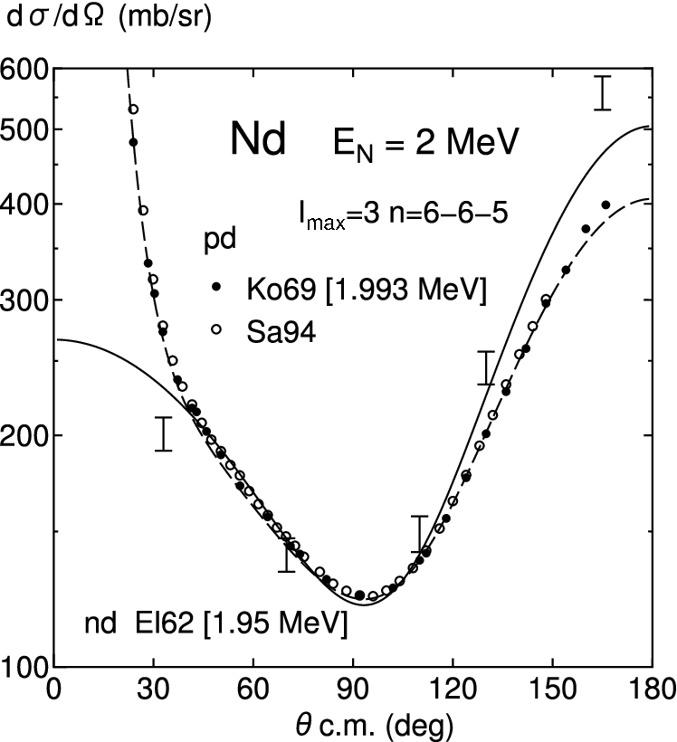
The vector analyzing-powers of the nucleon, predicted by model fss2, are shown in Figs. 1 and 2 for the neutron incident energies $E_{n}=3$ to 65 MeV. The calculations in this paper were carried out using the maximum angular momentum for the $NN$ system, $I_{\rm max}=3$ or 4, and the momentum mesh-points $n=5$ -6-5 or 6-6-5, in the definition defined in I. For the energies $E_{n}\leq 3$ MeV, the partial waves up to $I_{\rm max}=3$ are good enough. We should note that the polarization observables are more sensitive to the truncation of the model space than the differential cross sections. They are also very sensitive to the Coulomb effect in the present low-energy region. Almost all polarization data are for the $pd$ or $dp$ scattering and the detailed comparison with the experiment requires the introduction of the Coulomb force. Here we show with dashed curves preliminary results obtained by applying the Vincent and Phatak method[18] to the $pd$ scattering.²² 2 The details of this approach to the $pd$ scattering will be reported in a separate paper. See also Ref. \citenapfb05. The $pd$ calculations were made using the cut-off Coulomb potential with the the cut-off radius $R_{c}=9$ fm (for $E_{p}\leq 3$ MeV) or $R_{c}=8$ fm (for $E_{p}\geq 5$ MeV), together with $I_{\rm max}=3$ and $n=6$ -6-5. The $nd$ data shown with bars should therefore be compared with the solid curves, while the $pd$ data with circles and others correspond to the dashed curves. The cited paper for these experimental data is specified by two letters and double figures, which are short for the first author’s name and the publication year, respectively. In the forward angular region with $\theta_{\rm cm}\leq 30^{\circ}$ , the enhancement of $A_{y}$ for the $pd$ data is almost correctly reproduced by the Coulomb effect, although the reduction in $\theta_{\rm cm}=60^{\circ}$ - $120^{\circ}$ makes the agreement with the experiment worse at the energy region $E_{p}=3$ - 14 MeV. We find that the difference between the solid curves and the dashed curves gradually diminishes for higher energies except for the forward angles.

Refer to caption — Figure 1: The nucleon analyzing-power $A_{y}(\theta)$ of the $nd$ elastic scattering (solid curve) from $E_{n}=3$ to 19 MeV, compared with the experiment (bars). The $pd$ results with the cut-off Coulomb force are also shown by dashed curves, which should be compared with empty circles. The experimental data are taken from Refs. \citenMc94 for Mc94 ( $nd$ ), \citenSa94 for Sa94 ( $pd$ ), \citenTo91 for To91 ( $nd$ ), \citenHo87 for Ho87 ( $nd$ ), \citenNi98 for Ni98 ( $nd$ ), and \citenWe10 for We10 ( $nd$ ).

Table 1: Comparison of the maximum values of

A_{y}

and their positions

\theta_{\rm cm}

with the

nd

and

pd

experimental data. The ratio between the theory and experiment is also shown.

$E_{N}$	system	fss2		ratio	experiment		Ref.
(MeV)		$\theta_{\rm cm}$ (deg)	${A_{y}}_{\rm max}$		$\theta_{\rm cm}$ (deg)	${A_{y}}_{\rm max}$
2	$nd$	95	0.0341	0.81	95	0.042	\citenNe03 [1.9 MeV]
	$pd$	92	0.0320	0.973	95	0.0329	\citenSa94
2.5	$nd$	100	0.0412	$-$
	$pd$	98	0.0387	0.921	99	0.0420	\citenSa94
3	$nd$	104	0.0487	0.81	104	0.060	\citenMc94
	$pd$	103	0.0443	0.899	104	0.0493	\citenSa94
5	$nd$	116	0.0726	0.80	115	0.091	\citenTo91
	$pd$	113	0.0684	0.840	113	0.0814	\citenSa94
7	$nd$	118	0.104	$-$
	$pd$	119	0.0930	0.830	119	0.112	\citenSa94
9	$nd$	122	0.131	0.87	119	0.15	\citenTo91 [8.5 MeV]
	$pd$	123	0.118	0.831	122	0.142	\citenSa94
10	$nd$	124	0.144	0.85	126	0.17	\citenTo82
	$pd$	124	0.131	0.845	124	0.155	\citenSa94
12	$nd$	127	0.167	0.88	128	0.19	\citenNi98
	$pd$	127	0.155	0.856	126	0.181	\citenSa94
14	$nd$	129	0.185	0.84	130	0.22	\citenTo83 [14.1 MeV]
	$pd$	129	0.177	0.876	128	0.202	\citenSa94
18	$nd$	133	0.203	$-$
	$pd$	133	0.205	0.928	132	0.221	\citenSa94
19	$nd$	133	0.205	0.89	132	0.23	\citenWe10
	$pd$	134	0.208	$-$

Our results in Fig. 1 imply that the long-standing $A_{y}$ -puzzle for the large discrepancies between the theory and experiment in the energy region $E_{n}\leq 25$ MeV is not so serious as the AV18 potential,[14, 15, 16, 17] although the maximum peak height of $A_{y}$ is still too low. We compare in Table 1 the theoretical peak heights with the $nd$ experimental data and with the $pd$ data given in Ref. \citenSa94. The comparison of the no-Coulomb calculations implies that our results are about 80 - 90 $\%$ of the observed $nd$ data, although exact evaluation of the ratio is not easy due to the experimental errorbars. A similar amount of discrepancy is also seen in the comparison of the $pd$ data, but it has an apparent minimum around $E_{p}=7$ MeV of about 83 $\%$ . As an average in this energy region, the shortage of about 15 $\%$ is a fair estimate both for the $nd$ and $pd$ data, which is better than the rather constant discrepancy by AV18 potential at the $25\%$ level up to about 25 MeV.[17] (See Fig. 2 of Ref. \citenTo08.) Looking back to the old predictions by realistic separable potentials, $A_{y}(\theta)$ at some energies are very well reproduced.[39, 40, 41, 42, 43] Our QM $NN$ interaction fss2 and the separable potentials are both considered to have quite different off-shell properties from the meson-exchange potentials, that are characterized by the strong nonlocality of the interaction in the configuration space. For the energies $E_{p}=30$ - 65 MeV, there is no clear discrepancy of $A_{y}$ between the theory and experiment.

We should mention that the improvement of $A_{y}(\theta)$ is not achieved by the modification of the $\hbox{}^{3}P_{J}$ phase shifts of the $NN$ interaction, as claimed in early studies of this problem. Although $A_{y}(\theta)$ is very sensitive to these phase shifts, an artificial modification (of almost $10\%$ ) is far beyond acceptable from the modern phase shift analysis of the $NN$ interaction.[14, 15] Our $NN$ model fss2 reproduces the empirical $\hbox{}^{3}P_{J}$ phase shifts within the accuracy of one degree at the energies less than 300 MeV. (See Fig. 1 of Ref. \citenPPNP.) From the detailed phase shift analysis of the $pd$ scattering up to $E_{p}=10$ MeV, the authors of Ref. \citenTo02 claim that the $\hbox{}^{4}P_{1/2}$ and $\varepsilon_{{3/2}^{-}}$ eigenphase shifts should be affected by the $3N$ force, in order to improve $A_{y}(\theta)$ . In fact, the phase shift analysis of the $pd$ scattering is very ambiguous in this energy region, since so many complex parameters are involved. In Ref. \citenscl10, we have compared the $nd$ phase shifts with the phase shift analysis[22] at much lower energies less than 3 MeV and found that the desirable feature to reproduce the sufficient binding energy of the triton and the spin-doublet $nd$ scattering length $\hbox{}^{2}a_{nd}$ is achieved by the more attractive feature of the $\hbox{}^{2}S_{1/2}$ phase shift of fss2 than the AV18 potential, originating from the nonlocal description of the short-range repulsion. We can conjecture that a similar situation is taking place even for the higher energies, although it is difficult to pinpoint some particular eigenphase shifts.

3.2 Vector and tensor analyzing-powers of the deuteron

We show the vector analyzing-powers of the deuteron in Fig. 3, and the tensor analyzing-powers in Figs. 4 - 6. All of these observables are measured from the $dp$ elastic scattering using the polarized deuteron, and discussion including the Coulomb force is definitely necessary for the comparison between the theory and experiment. The introduction of the Coulomb force to the vector analyzing-power $iT_{11}$ in Fig. 3, shown with the dashed curves leads to the enhancement at $\theta_{\rm cm}\leq 30^{\circ}$ and the reduction at $\theta_{\rm cm}=80^{\circ}$ - $120^{\circ}$ for the low-energies $E_{p}=3$ - 9 MeV, that are very similar to the situation of $A_{y}$ . We have unpleasant rise of the hill at the angular region $\theta_{\rm cm}=20^{\circ}$ - $90^{\circ}$ for the energies $E_{p}=3$ - 10 MeV, which is probably related to the inadequacy of the nuclear-Coulomb interference term. The peak height around $\theta_{\rm cm}=120^{\circ}$ is somewhat too low at $E_{p}=3$ - 9 MeV, although it is not so serious as in Fig. 5 of Ref. \citenKi01. Except for these, there is no clear discrepancies between the theory and experiment. As to the first problem, the enhancement by the Coulomb effect is also seen in other calculations by Berthold et al.[20], Alt et al.[21], Kievsky et al.[23] and Deltuva et al.[24, 25], although to less extent in the last two cases. It is possible that the corresponding $nd$ quantities are too large.

The tensor-type analyzing-powers $T_{20},~T_{21}$ and $T_{22}$ for the energies $E_{p}=3$ and 5 MeV in Fig. 4 show a fairly large Coulomb effect in the whole angles. In particular, the forward behavior of $T_{20}$ and $T_{21}$ in $\theta_{\rm cm}\leq 60^{\circ}$ for the no-Coulomb calculation (solid curves) is entirely modified by the Coulomb effect, resulting in a good agreement with the $dp$ experimental data. We have some problems with $T_{20}$ and $T_{21}$ in the angular region $\theta_{\rm cm}=20^{\circ}$ - $70^{\circ}$ for the energies $E_{p}=7$ - 9 MeV, which might again related to the nuclear-Coulomb interference. In $T_{22}$ , too large negative values at the minimum points are shifted to the smaller direction, giving better reproduction of the experimental data. On the low-energy side with $E_{p}\leq 3$ MeV, the minimum points of the dips are slightly too high. Related to this, the perfect fit of $T_{22}$ in Ref. \citenPREP at $E_{\rm lab}\leq 10$ MeV is fortuitous, because this calculation does not include the Coulomb force. The Coulomb modification diminishes smaller and smaller for the higher energies $E_{p}=7$ and 9 MeV in Fig. 5, and for $E_{p}=22.7$ and 65 MeV in Fig. 6. The big difference from the experiment in 65 MeV $T_{21}$ at $\theta_{\rm cm}=50^{\circ}$ - $90^{\circ}$ is a common feature with other calculations.[10] In order to examine the adequacy of our Coulomb treatment, we have compared our Coulomb effects with the results of calculations by other authors.[20, 21, 24, 25, 23, 26] For example, Ref. \citenDe05 shows the differential cross sections and analyzing-powers of $E_{p}=3$ and 9 MeV in Figs. 9 and 10, respectively, for the coupled-channel potentials of CD Bonn, including the

$\Delta$ degree of freedom. We find that the general tendency is common, although some quantitative differences exist because of the different treatments of the Coulomb force.

3.3 Analysis of the Coulomb effect below the deuteron breakup threshold

In our previous paper,[13] we have examined the Coulomb effect on the $pd$ differential cross sections for the incident energies below the deuteron breakup threshold. In this low-energy region, the channel spin $S_{c}$ is an almost good quantum number, and the $J$ -averaging of the eigenphase shifts with respect to the definite $S_{c}$ and the orbital angular momentum $\ell$ between the nucleon and the deuteron is very convenient to reduce the number of phase shift parameters, at least in discussing the angular distribution of differential cross sections. However, a simple prescription adding the Coulomb amplitude to the $nd$ scattering amplitude only with the Coulomb phase-shift factors, which is called the “Coulomb externally corrected” approximation in Ref. \citenDe05, does not work for the differential cross sections in the low-energy region. This prescription largely overestimates the differential cross sections. This implies that the modification of the nuclear phase shifts by the Coulomb force is very important below the deuteron breakup threshold. In Ref. \citenscl10, the Coulomb modification to the nuclear phase shifts is therefore incorporated, using the difference of the $J$ -averaged eigenphase shifts for the $nd$ and $pd$ scatterings first from the AV18 potential in Ref. \citenKi96, secondly from the fss2 calculated here. In both cases, we have obtained an almost complete reproduction of the differential cross sections by this prescription.

Here, we incorporate the Coulomb force by the Vincent and Phatak method, directly to the nuclear scattering amplitudes. The results are shown by dashed curves in Figs. 7 - 9. We find that the $pd$ or $dp$ experimental data are generally well reproduced. In more detail, we find the following two problems:

1)

The $A_{y}$ puzzle is more serious below the deuteron breakup threshold, especially for the $nd$ data. For instance, the recent $A_{y}$ measurement of the low-energy $nd$ scattering in Ref. \citenNe03 shows the discrepancy of more than $30\%$ , although the difference in the $pd$ case is not so serious.
2)

The minimum points in the deuteron tensor analyzing-power $T_{22}$ are too high, which is a common feature with the 3 MeV result in Fig. 4.

We can compare our results with those by the variational approach in Ref. \citenKi96, which incorporates the complete Coulomb force to the AV18 potential and the Urbana three-nucleon force. The AV18 potential yields particularly large discrepancy of more than $30\%$ in this energy region not only for $A_{y}$ but also for $iT_{11}$ , as seen in Figs. 1 and 2 in Ref. \citenKi96. The differential cross sections and the tensor-type deuteron analyzing-powers $T_{2m}$ are well reproduced. As to the difference in $T_{22}$ in 2) above, the comparison with their results indicates that the three-body force might be important to reproduce the magnitude at the minimum points. The deuteron analyzing-powers, $iT_{11}$ and $T_{2m}$ , at $E_{d}=3$ MeV in Fig. 8 are very similar to their results in Fig. 12 of Ref. \citenKi96, although the comparison with the experimental data is not easy because of the experimental errorbars.

3.4 Polarization transfer coefficients

The nucleon polarization transfer coefficients $K^{\beta^{\prime}}_{\alpha}(\theta)$ of the $nd$ elastic scattering are compared with the $pd$ data for $E_{n}=10$ MeV and 22.7 MeV in Fig. 10. The dotted curves represent the kinematical rotation in Eq. (73) when $K_{\alpha,\beta}=\delta_{\alpha,\beta}$ is assumed. From here on, we neglect the Coulomb effect and compare the $nd$ results directly with the $pd$ data. This would be permissible since the experimental errorbars are still large for these polarization observables. We find satisfactory agreement between the theory and experiment. The vector-type nucleon to deuteron polarization transfer coefficients $K^{\beta^{\prime}}_{\alpha}(\theta)$ are compared in Fig. 11 at the same energies $E_{n}=10$ and 22.7 MeV. The dotted curves again represent the kinematical rotation in Eq. (77) when $K_{\alpha,\beta}=\delta_{\alpha,\beta}$ is assumed. Various types of the nucleon to deuteron polarization transfer coefficients are compared with the $pd$ data in Figs. 12 - 14. Here, again we obtain satisfactory agreement although the experimental errorbars are rather large.

3.5 Spin correlation coefficients

The spin correlation coefficients, $C_{xx},~C_{yy}$ , and $S=(-1/2)C^{yy}_{y}$ , for the $nd$ elastic scattering at $E_{n}=8.7$ , 10, 12 and 13 MeV are compared with the $pd$ experimental data in Figs. 15 and 16. The experimental data are actually for the $dp$ scattering at the energies $E_{d}=17.4$ , 19.5, 23.8 and 26.1 MeV.[64] We find a reasonable agreement between the theory and experiment, although the experimental errorbars are rather large.

4 Summary

One of the most important purposes of studying the three-nucleon ( $3N$ ) system in terms of realistic nucleon-nucleon ( $NN$ ) interactions is to clarify the off-shell properties of the interaction, which can never be known from the physical observables of the two-nucleon system. It is therefore very crucial that the $NN$ interaction to start with can reproduce the deuteron properties and the $NN$ phase shifts very accurately. Our quark-model $NN$ interaction fss2 satisfies this criterion by taking into account the naive three-quark structure of the nucleon. It is formulated in the framework of the resonating-group method (RGM), in which the antisymmetrization of quarks generates a strong nonlocality and characteristic energy dependence of the interaction between two three-quark clusters. When this interaction is applied to the $3N$ system, the short-range repulsion originating from this nonlocality behaves quite differently from the meson-exchange potentials in favor of the deuteron distortion in the spin-doublet channel. We have found that fss2 yields sufficient attraction comparable to the AV18 plus Urbana $3N$ force, leading to the nearly correct triton binding energy and the empirical value of the spin-doublet effective length for the $nd$ interaction.[13] Note that this strong deuteron distortion effect is only for the $J^{\pi}=1/2^{+}$ channel. On the other hand, the distortion effect is marginal in the spin quartet channel or the $J^{\pi}=3/2^{+}$ channel, owing to the Pauli principle on the nucleon level. As the result, the eigenphase shift of the dominant $\hbox{}^{4}S_{3/2}$ state predicted by fss2 is very similar to the AV18 potential, in which the effect of $3N$ force is very small. In the low-energy region, the effect of the $3N$ force hardly appears since the differential cross sections are dominated by the partial waves of the spin-quartet channel. It is important to note that fss2 can also reproduce the differential cross sections at higher energies, including the sufficient magnitude of the cross sections at the diffraction minima.[4]

In this paper, we have extended the previous studies,[4, 13] applying fss2 to the $nd$ elastic scattering, to various types of polarization observables. The long-standing $A_{y}$ -puzzle [14, 15, 16, 17] for the nucleon vector analyzing-powers in the low-energy region $E_{n}\leq 25$ MeV is largely improved in comparison with the predictions by the AV18 potential. Although the Coulomb effect obscures the definite conclusion, the shortage of the maximum peak is about 15 $\%$ , which is somewhat similar to the predictions by old realistic separable potentials.[43, 41, 42] The detailed comparison with the phase shift analysis is not possible since the empirical phase shifts are not uniquely determined. Nevertheless, the conclusion drawn in Ref. \citenTo02 based on the solutions derived from the AV18 potential should be reconsidered, since $\hbox{}^{2}P_{J}$ phase shifts at the energy $E_{p}\sim 10$ MeV are quite different between fss2 and the AV18 potential. The difference is of the order of several degrees. It is possible that this difference is caused by the nonlocality of the quark-model $NN$ interaction. Since all the experimental data for the deuteron analyzing-powers are for the $pd$ or $dp$ scattering, we have introduced the cut-off Coulomb force by the Vincent and Phatak method. This method works very well to reproduce the behavior of the differential cross sections and analyzing-powers at the forward angles. In particular, the low-energy observables below the deuteron breakup threshold are well reproduced except for the $A_{y}$ -puzzle and a slight underestimation of the dips in $T_{22}(\theta)$ at the minimum points around $\theta_{\rm cm}=100^{\circ}$ - $120^{\circ}$ . A large discrepancy of the vector-type analyzing-power of the deuteron, $iT_{11}(\theta)$ , found in Ref. \citenKi01 is not observed in our calculations, although the peak height around $\theta_{\rm cm}=120^{\circ}$ is somewhat too low at $E_{p}=3$ - 9 MeV. Instead, we have unpleasant rise of the hill at the angular region $\theta_{\rm cm}=20^{\circ}$ - $90^{\circ}$ for the energies $E_{p}=5$ - 10 MeV, which is probably related to the inadequacy of the nuclear-Coulomb interference term in our Coulomb treatment. A similar problem is also seen in $T_{20}$ and $T_{21}$ in the angular rigion $\theta_{\rm cm}=20^{\circ}$ - $70^{\circ}$ for the energies $E_{p}=7$ - 9 MeV. Except for these, there is no clear discrepancies between the theory and experiment. We have carefully examined the Coulomb effect on the observables between our results and other calculations using the modern meson exchange potentials like AV18 and CD Bonn potentials.[23, 24, 25, 26] The direction of the Coulomb modification is always the same, although some quantitative diference appears at the forward angles. Our calculation somehow overestimates the Coulomb effect and nuclear-Coulomb interference term is not precisely reproduced. On the other hand, the behavior of the observables in the backward angles $\theta_{\rm cm}\gg 90^{\circ}$ is hardly influenced especially at higher energies $E_{p}>10$ MeV. We have also examined various types of polarization transfer coefficients and the spin correlation coefficients by neglecting the Coulomb force. They are reasonably reproduced, although the experimental errorbars are still very large.

In conclusion, we find no apparent disagreement between the theory and experiment as far as $nd$ elastic scattering with the energies $E_{n}\leq 65$ MeV is concerned. It should be stressed that this conclusion is valid only when we deal with the energy dependence of the quark-model RGM kernel properly.[65, 66] As discussed in our previous paper,[4] this energy dependence is eliminated by the standard off-shell transformation utilizing the square root of the normalization kernel. This procedure yields an extra nonlocal kernel which is not extremely small and affects various $3N$ observables in different ways. In the next paper, we will discuss the deuteron breakup processes.[67]

Acknowledgements

The authors would like to thank Professors K. Miyagawa, H. Witała, H. Kamada and S. Ishikawa for many useful comments. We also thank Professor K. Sagara for providing us the $pd$ experimental data by the Kyushu university group. This work was supported by the Grant-in-Aid for Scientific Research on Priority Areas (Grant No. 20028003), and by the Grant-in-Aid for the Global COE Program “The Next Generation of Physics, Spun from Universality and Emergence” from the Ministry of Education, Culture, Sports, Science and Technology (MEXT) of Japan. It was also supported by the core-stage backup subsidies of Kyoto University. The numerical calculations were carried out on Altix3700 BX2 at YITP in Kyoto University and on the high performance computing system, Intel Xeon X5680, at RCNP in Osaka University.

Appendix A Spin operators of the deuteron

In this appendix, we summarize various notations for the spin operators of the deuteron. The deuteron spin operators are most easily defined from the Wigner-Eckart theorem

\displaystyle\langle 1m^{\prime}|S_{\mu}|1m\rangle=\langle 1m1\mu|1m^{\prime}\rangle\langle 1||{\hbox{\boldmath$S$}}||1\rangle_{\rm unc}\ ,

(102)

with the standard value of the reduce matrix element $\langle 1||{\hbox{\boldmath$S$}}||1\rangle_{\rm unc}=\sqrt{1\cdot 2}$ . Here, the subscript “unc” stands for the unconventional reduced matrix element with $\langle S||{\hbox{\boldmath$S$}}||S\rangle_{\rm unc}=\sqrt{S(S+1)}$ . This gives the rank-one spin operator of the deuteron as

	$\displaystyle S_{1}=-\left(\begin{array}[]{ccc}0&1&0\\ 0&0&1\\ 0&0&0\\ \end{array}\right),\quad S_{0}=\left(\begin{array}[]{ccc}1&0&0\\ 0&0&0\\ 0&0&-1\\ \end{array}\right),\quad S_{-1}=\left(\begin{array}[]{ccc}0&0&0\\ 1&0&0\\ 0&1&0\\ \end{array}\right)=-{S_{1}}^{\dagger}.$
			(113)

The transformation to the Cartesian representation is carried out by the standard spherical vector representation:

\displaystyle\begin{array}[]{l}S_{1}=-\frac{1}{\sqrt{2}}\left(S_{x}+iS_{y}\right)\\[5.69054pt] S_{0}=S_{z}\\[5.69054pt] S_{-1}=\frac{1}{\sqrt{2}}\left(S_{x}-iS_{y}\right)\\ \end{array}\ \ ,\qquad\begin{array}[]{l}S_{x}=\frac{1}{\sqrt{2}}\left(-S_{1}+S_{-1}\right)\\[5.69054pt] S_{y}=i\,\frac{1}{\sqrt{2}}\left(S_{1}+S_{-1}\right)\\[5.69054pt] S_{z}=S_{0}\\ \end{array}\ ,

which yields

	$\displaystyle S_{x}=\frac{1}{\sqrt{2}}\left(\begin{array}[]{ccc}0&1&0\\ 1&0&1\\ 0&1&0\\ \end{array}\right),\quad S_{y}=\frac{i}{\sqrt{2}}\left(\begin{array}[]{ccc}0&-1&0\\ 1&0&-1\\ 0&1&0\\ \end{array}\right),\quad S_{z}=\left(\begin{array}[]{ccc}1&0&0\\ 0&0&0\\ 0&0&-1\\ \end{array}\right).$
			(131)

Note that ${\hbox{\boldmath$S$}}^{\dagger}={\hbox{\boldmath$S$}}$ and ${\hbox{\boldmath$S$}}^{2}=2$ , which is consistent with the reduced matrix element. The rank-two spin operator of the deuteron is defined by $S^{(2)}_{m}=[SS]^{(2)}_{m}$ and the reduced matrix element is calculated from

\displaystyle\langle 1m^{\prime}|S^{(2)}_{\mu}|1m\rangle=\langle 1m2\mu|1m^{\prime}\rangle\langle 1||S^{(2)}||1\rangle_{\rm unc}\ .

(132)

We note that the spin operator $S$ does not change the spin value $S=1$ , when it is operated on the deuteron spin wave function $\chi_{1}=\chi_{1}(12)$ :

\displaystyle S|\chi_{1}\rangle_{(11)1\mu}=-[S\chi_{1}]_{1\mu}=\sqrt{2}\chi_{1\mu}\ .

(133)

(Note the phase change by the angular-momentum coupling order.) We find

	$\displaystyle S^{(2)}\|\chi_{1}\rangle_{(12)1\mu}=[S^{(2)}\chi_{1}]_{1\mu}=[[SS]_{2}\chi_{1}]_{1\mu}=\sum_{\lambda=0,1,2}\left[\begin{array}[]{ccc}1&1&2\\[5.69054pt] 0&1&1\\[5.69054pt] 1&\lambda&1\\ \end{array}\right][S[S\chi_{1}]_{\lambda}]_{1\mu}$
	$\displaystyle=\left[\begin{array}[]{ccc}1&1&2\\[5.69054pt] 0&1&1\\[5.69054pt] 1&1&1\\ \end{array}\right](-\sqrt{2})[S\chi_{1}]_{1\mu}=\sqrt{15}\left\{\begin{array}[]{ccc}2&1&1\\ 1&1&1\\ \end{array}\right\}(-\sqrt{2})(-\sqrt{2})\chi_{1\mu}$
	$\displaystyle=\sqrt{15}\frac{1}{6}(-\sqrt{2})(-\sqrt{2})=\sqrt{\frac{5}{3}}\chi_{1\mu}\ ,$		(144)

which yields

\displaystyle\langle 1||S^{(2)}||1\rangle=\sqrt{\frac{5}{3}}\ .

(145)

This value and Eq. (132) gives

\displaystyle\langle 1m^{\prime}|S^{(2)}_{\mu}|1m\rangle=(-)^{1-m}\langle 1m^{\prime}1-m|2\mu\rangle\ ,

(146)

owing to the symmetry property of the CG coefficients. The explicit values of the CG coefficients

	$\displaystyle\langle 1111\|22\rangle=1\ ,\quad\langle 1110\|21\rangle=\frac{1}{\sqrt{2}}\ ,\quad\langle 1010\|20\rangle=\sqrt{\frac{2}{3}}\ ,\quad\langle 11~1,\,-1\|20\rangle=\frac{1}{\sqrt{6}}\ ,$
			(147)

and other non-zero coefficients obtained by the symmetries, yield

	$\displaystyle S^{(2)}_{2}=\left(\begin{array}[]{ccc}0&0&1\\ 0&0&0\\ 0&0&0\\ \end{array}\right)\ ,\quad S^{(2)}_{-2}=\left(\begin{array}[]{ccc}0&0&0\\ 0&0&0\\ 1&0&0\\ \end{array}\right)={S^{(2)}_{2}}^{\dagger},$
	$\displaystyle S^{(2)}_{1}=\frac{1}{\sqrt{2}}\left(\begin{array}[]{ccc}0&-1&0\\ 0&0&1\\ 0&0&0\\ \end{array}\right)\ ,\quad S^{(2)}_{-1}=\frac{1}{\sqrt{2}}\left(\begin{array}[]{ccc}0&0&0\\ 1&0&0\\ 0&-1&0\\ \end{array}\right)=-{S^{(2)}_{1}}^{\dagger},$
	$\displaystyle S^{(2)}_{0}=\frac{1}{\sqrt{6}}\left(\begin{array}[]{ccc}1&0&0\\ 0&-2&0\\ 0&0&1\\ \end{array}\right)\ .$

The transformation to the Cartesian representation is carried out by using a general formula which is obtained from the CG coefficients Eq. (147) and the vector-tensor transformation Eq. (A). Namely, for two vectors $a$ and $b$ we have

	$\displaystyle[ab]_{22}+[ab]_{2-2}=a_{x}b_{x}-a_{y}b_{y}\ \,\qquad[ab]_{22}-[ab]_{2-2}=i(a_{x}b_{y}+a_{y}b_{x})\ ,$
	$\displaystyle[ab]_{21}+[ab]_{2-1}=-i(a_{y}b_{z}+a_{z}b_{y})\ \,\qquad[ab]_{21}-[ab]_{2-1}=-(a_{x}b_{z}+a_{z}b_{x})\ ,$
	$\displaystyle[ab]_{20}=\frac{1}{\sqrt{6}}\left(2a_{z}b_{z}-a_{x}b_{x}-a_{y}b_{y}\right)\ .$		(166)

If we set ${\hbox{\boldmath$a$}}={\hbox{\boldmath$b$}}={\hbox{\boldmath$S$}}$ , we find

	$\displaystyle S^{(2)}_{2}+S^{(2)}_{-2}={S_{x}}^{2}-{S_{y}}^{2}\ ,\qquad S^{(2)}_{2}-S^{(2)}_{-2}=i(S_{x}S_{y}+S_{y}S_{x})\ ,$
	$\displaystyle S^{(2)}_{1}+S^{(2)}_{-1}=-i(S_{y}S_{z}+S_{z}S_{y})\ \,\qquad S^{(2)}_{1}-S^{(2)}_{-1}=-(S_{x}S_{z}+S_{z}S_{x})\ ,$
	$\displaystyle S^{(2)}_{0}=\frac{1}{\sqrt{6}}\left(2{S_{z}}^{2}-{S_{x}}^{2}-{S_{y}}^{2}\right)\ .$		(167)

Here we should note that the deuteron spin operator $S$ satisfies the commutation relations

\displaystyle\left[S_{\alpha},S_{\beta}\right]=i\sum_{\gamma}\varepsilon_{\alpha\beta\gamma}S_{\gamma}\ .

(168)

We use this relationship and define the spin operators of the deuteron in the Cartesian representation ${\cal P}_{\alpha\beta}$ , following the definition by Ohlsen (see Eq. (2.17) of Ref. \citenOh72.) Namely, we define ${\cal P}_{\alpha}=S_{\alpha}$ and

	$\displaystyle{\cal P}_{xy}=\frac{3}{2}\left(S_{x}S_{y}+S_{y}S_{x}\right)\ \ ,\qquad{\cal P}_{xz}=\frac{3}{2}\left(S_{x}S_{z}+S_{z}S_{x}\right)\ ,$
	$\displaystyle{\cal P}_{yz}=\frac{3}{2}\left(S_{y}S_{z}+S_{z}S_{y}\right)\ .$		(169)

For the diagonal part ${\cal P}_{\alpha\alpha}$ , we define ${\cal P}_{\alpha\alpha}=3{S_{\alpha}}^{2}-2$ symmetrically, which leads to ${\cal P}_{xx}+{\cal P}_{yy}+{\cal P}_{zz}=0$ , owing to ${\hbox{\boldmath$S$}}^{2}=2$ . We also use the normalized tensor operators of the deuteron $T_{1\mu}$ and $T_{2\mu}$ defined by

\displaystyle T_{1\mu}=\sqrt{\frac{3}{2}}~S_{\mu}\ \ ,\qquad T_{2\mu}=\sqrt{3}~S^{(2)}_{\mu}\ ,

(170)

which satisfy

\displaystyle{T_{\kappa\nu}}^{\dagger}=(-)^{\nu}T_{\kappa-\nu}\ \ ,\qquad\frac{1}{3}Tr\left(T_{\kappa\nu}\,T^{\dagger}_{\kappa^{\prime}\nu^{\prime}}\right)=\delta_{\kappa,\kappa^{\prime}}\delta_{\nu,\nu^{\prime}}\ .

(171)

The Glöckle et al.’s review article [10] also uses the notation $S^{(i)}$ ( $i=0$ - 8) for $T_{\kappa\nu}$ , which satisfy

\displaystyle{S^{(i)}}^{\dagger}=S^{(i)}\ \ ,\qquad\frac{1}{3}Tr\left(S^{(i)}\,S^{(j)}\right)=\delta_{i,j}\ .

(172)

All of these different notations are related by

	$\displaystyle S^{(0)}=1\ ,$
	$\displaystyle S^{(1)}=\sqrt{\frac{3}{2}}{\cal P}_{x}=\sqrt{\frac{3}{2}}S_{x}=\frac{\sqrt{3}}{2}\left(\begin{array}[]{ccc}0&1&0\\ 1&0&1\\ 0&1&0\\ \end{array}\right)\ ,$
	$\displaystyle S^{(2)}=\sqrt{\frac{3}{2}}{\cal P}_{y}=\sqrt{\frac{3}{2}}S_{y}=i\,\frac{\sqrt{3}}{2}\left(\begin{array}[]{ccc}0&-1&0\\ 1&0&-1\\ 0&1&0\\ \end{array}\right)\ ,$
	$\displaystyle S^{(3)}=\sqrt{\frac{3}{2}}{\cal P}_{z}=\sqrt{\frac{3}{2}}S_{z}=\sqrt{\frac{3}{2}}\left(\begin{array}[]{ccc}1&0&0\\ 0&0&0\\ 0&0&-1\\ \end{array}\right)\ ,$
	$\displaystyle S^{(4)}=\sqrt{\frac{2}{3}}{\cal P}_{xy}=\sqrt{\frac{2}{3}}\frac{3}{2}\left(S_{x}S_{y}+S_{y}S_{x}\right)=i\,\sqrt{\frac{3}{2}}\left(\begin{array}[]{ccc}0&0&-1\\ 0&0&0\\ 1&0&0\\ \end{array}\right)\ ,$
	$\displaystyle S^{(5)}=\sqrt{\frac{2}{3}}{\cal P}_{yz}=\sqrt{\frac{2}{3}}\frac{3}{2}\left(S_{y}S_{z}+S_{z}S_{y}\right)=i\,\frac{\sqrt{3}}{2}\left(\begin{array}[]{ccc}0&-1&0\\ 1&0&1\\ 0&-1&0\\ \end{array}\right)\ ,$
	$\displaystyle S^{(6)}=\sqrt{\frac{2}{3}}{\cal P}_{xz}=\sqrt{\frac{2}{3}}\frac{3}{2}\left(S_{x}S_{z}+S_{z}S_{x}\right)=\frac{\sqrt{3}}{2}\left(\begin{array}[]{ccc}0&1&0\\ 1&0&-1\\ 0&-1&0\\ \end{array}\right)\ ,$
	$\displaystyle S^{(7)}=\frac{1}{\sqrt{6}}\left({\cal P}_{xx}-{\cal P}_{yy}\right)=\frac{1}{\sqrt{6}}3\left({S_{x}}^{2}-{S_{y}}^{2}\right)=\sqrt{\frac{3}{2}}\left(\begin{array}[]{ccc}0&0&1\\ 0&0&0\\ 1&0&0\\ \end{array}\right)\ ,$
	$\displaystyle S^{(8)}=\frac{1}{\sqrt{2}}{\cal P}_{zz}=\frac{1}{\sqrt{2}}\left(3{S_{z}}^{2}-2\right)=\frac{1}{\sqrt{2}}\left(\begin{array}[]{ccc}1&0&0\\ 0&-2&0\\ 0&0&1\\ \end{array}\right)\ .$
			(205)

The relationship between the tensor notation and $S^{(i)}$ is

	$\displaystyle S^{(2)}_{2}=\frac{1}{\sqrt{6}}\left(S^{(7)}+iS^{(4)}\right)\ \ ,\qquad S^{(2)}_{-2}=\frac{1}{\sqrt{6}}\left(S^{(7)}-iS^{(4)}\right)\ ,$
	$\displaystyle S^{(2)}_{1}=-\frac{1}{\sqrt{6}}\left(S^{(6)}+iS^{(5)}\right)\ \ ,\qquad S^{(2)}_{-1}=\frac{1}{\sqrt{6}}\left(S^{(6)}-iS^{(5)}\right)\ ,$
	$\displaystyle S^{(2)}_{0}=\frac{1}{\sqrt{3}}S^{(8)}\ ,$		(206)

	$\displaystyle T_{00}=S^{(0)}=1\ ,$
	$\displaystyle T_{11}=-\frac{1}{\sqrt{2}}\left(S^{(1)}+iS^{(2)}\right)\ \ ,\qquad T_{1,-1}=\frac{1}{\sqrt{2}}\left(S^{(1)}-iS^{(2)}\right)\ ,$
	$\displaystyle T_{10}=S^{(3)}\ ,$
	$\displaystyle T_{22}=\frac{1}{\sqrt{2}}\left(S^{(7)}+iS^{(4)}\right)\ \ ,\qquad T_{2,-2}=\frac{1}{\sqrt{2}}\left(S^{(7)}-iS^{(4)}\right)\ ,$
	$\displaystyle T_{21}=-\frac{1}{\sqrt{2}}\left(S^{(6)}+iS^{(5)}\right)\ \ ,\qquad T_{2,-1}=\frac{1}{\sqrt{2}}\left(S^{(6)}-iS^{(5)}\right)\ ,$
	$\displaystyle T_{20}=S^{(8)}\ .$		(207)

If we express these by ${\cal P}_{\alpha}$ and ${\cal P}_{\alpha\beta}$ , we obtain

	$\displaystyle i\frac{1}{2}\left(T_{11}+T_{1,-1}\right)=\frac{\sqrt{3}}{2}{\cal P}_{y}\ \ ,\qquad T_{20}=\frac{1}{\sqrt{2}}{\cal P}_{zz}\ ,$
	$\displaystyle\frac{1}{2}\left(T_{21}-T_{2,-1}\right)=-\frac{1}{\sqrt{3}}{\cal P}_{xz}\ \ ,\qquad\frac{1}{2}\left(T_{22}+T_{2,-2}\right)=\frac{1}{2\sqrt{3}}\left({\cal P}_{xx}-{\cal P}_{yy}\right)\ ,$		(208)

where the other components of the deuteron analyzing-powers are zero as in $\lx@sectionsign\,2.2$ .

References

[1] Y. Fujiwara, Y. Suzuki and C. Nakamoto, \JLProg. Part. Nucl. Phys.,58,2007,439.
[2] Y. Suzuki, H. Matsumura, M. Orabi, Y. Fujiwara, P. Descouvemont, M. Theeten and D. Baye, \PLB659,2008,160.
[3] Y. Fujiwara, K. Miyagawa, M. Kohno, Y. Suzuki and H. Nemura, \PRC66,2002,021001(R); Y. Fujiwara, K. Miyagawa, M. Kohno and Y. Suzuki, \PRC70,2004,024001; Y. Fujiwara, Y. Suzuki, M. Kohno and K. Miyagawa, \PRC77,2008,027001.
[4] Y. Fujiwara and K. Fukukawa, \PTP124,2010,433.
[5] E. O. Alt, P. Grassberger and W. Sandhas, \NPB2,1967,167.
[6] H. P. Noyes, \PRL15,1965,538.
[7] K. L. Kowalski, \PRL15,1965,798; Errata 15 (1965), 908.
[8] W. Glöckle, G. Hasberg and A. R. Neghabian, \JLZ. Phys. A,305,1982,217.
[9] H. Witała, Th. Cornelius and W. Glöckle, \JLFew-Body Systems,3,1988,123.
[10] W. Glöckle, H. Witała, D. Hüber, H. Kamada and J. Golak, \JLPhysics Reports,274,1996,107.
[11] H. Liu, Ch. Elster and W. Glöckle, \PRC72,2005,054003.
[12] K. Fukukawa, Y. Fujiwara and Y. Suzuki, \JLMod. Phys. Lett. A,24,2009,1035.
[13] K. Fukukawa and Y. Fujiwara, arXiv: nucl-th1010.2024, submitted to Prog. Theor. Phys. (2010).
[14] W. Tornow and H. Witała, \NPA637,1998,280.
[15] W. Tornow, H. Witała and A. Kievsky, \PRC57,1998,555.
[16] W. Tornow, A. Kievsky and H. Witała, \JLFew-Body Systems,32,2002,53.
[17] W. Tornow, J. H. Esterline and G. J. Weisel, \JLJ. Phys. G: Nucl. Part. Phys.,35,2008,125104.
[18] C. M. Vincent and S. C. Phatak, \PRC10,1974,391.
[19] Y. Fujiwara, in Proceedings of the Third Asia-Pacific Conference on Few-Body Problems in Physics (APFB05), World Scientific Co. Ltd., 2007, pp. 221 - 225.
[20] G. H. Berthold, A. Stadler and H. Zankel, \PRC41,1990,1365.
[21] E. O. Alt, A. M. Mukhamedzhanov, M. M. Nishonov and A. I. Sattarov, \PRC65,2002,064613
[22] A. Kievsky, S. Rosati, W. Tornow and M. Viviani, \NPA607,1996,402.
[23] A. Kievsky, M. Viviani and S. Rosati, \PRC64,2001,024002.
[24] A. Deltuva, A. C. Fonseca and P. U. Sauer, \PRC71,2005,054005.
[25] A. Deltuva, A. C. Fonseca, A. Kievsky, S. Rosati, P. U. Sauer and M. Viviani, \PRC71,2005,064003.
[26] S. Ishikawa, \PRC80,2009,054002, and private communications.
[27] J. M. Blatt and L. C. Biedenharn, \JLRev. Mod. Phys.,24,1952,258.
[28] T. Fujita, Y. Fujiwara, C. Nakamoto and Y. Suzuki, \PTP100,1998,931.
[29] G. G. Ohlsen, \JLRep. Prog. Phys.,35,1972,717.
[30] J. E. McAninch, L. O. Lamm and W. Haeberli, \PRC50,1994,589.
[31] K. Sagara, H. Oguri, S. Shimizu, K. Maeda, H. Nakamura, T. Nakashima and S. Morinobu, \PRC50,1994,576.
[32] W. Tornow, C. R. Howell, M. Alohali, Z. P. Chen, P. D. Felsher, J. M. Hanly, R. L. Walter, G. Weisel, G. Mertens, I. Šlaus, H. Witała and G. Glöckle, \PLB257,1991,273.
[33] C. R. Howell, W. Tornow, K. Murphy, H. G. Pfützner, M. L. Roberts, Anli Li, P. D. Felsher, R. L. Walter, I. Šlaus, P. A. Treado and Y. Koike, \JLFew-Body Systems,2,1987,19.
[34] N. Nishimori, K. Sagara, T. Fujita, F. Wakamatsu, T. Bussaki, K. Maeda, H. Akiyoshi, K. Tsuruta, H. Nakamura and T. Nakashima, \NPA631,1998,697c.
[35] E. M. Neidel, W. Tornow, D. E. González Trotter, C. R. Howell, A.S. Crowell, R. A. Macri, R. L. Walter, G. J. Weisel, J. Esterline, H. Witała, B. J. Crowe III, R. S. Pedroni and D. M. Markoff, \PLB552,2003,29.
[36] W. Tornow, C. R. Howell, R. C. Byrd, R. S. Pedroni and R. L. Walter, \PRL49,1982,312.
[37] W. Tornow, R. C. Byrd, C. R. Howell, R. S. Pedroni and R. L. Walter, \PRC27,1983,2439.
[38] G. J. Weisel, W. Tornow, B. J. Crowe III, A. S. Crowell, J. H. Esterline, C. R. Howell, J. H. Kelley, R. A. Macri, R. S. Pedroni, R. L. Walter and H. Witała, \PRC81,2010,024003.
[39] P. Doleschall, W. Grüebler, V. König, P. A. Schmelzbach, F. Sperisen, and B. Jenny, \NPA380,1982,72.
[40] M. Sawada, S. Seki, K. Furuno, Y. Tagishi, Y. Nagashima, J. Schimizu, M. Ishikawa, T. Sugiyama, L. S. Chuang, W. Grüebler, J. Sanada, Y. Koike and Y. Taniguchi, \PRC27,1983,1932.
[41] Y. Koike and J. Haidenbauer, \NPA463,1987,365c.
[42] Y. Koike, J. Haidenbauer and W. Plessas, \PRC35,1987,396.
[43] G. Rauprich, H. J. Hähn, M. Karus, P. Nießen, K. R. Nyga, H. Oswald, L. Sydow, H. Paetz gen. Schieck and Y. Koike, \JLFew-Body Systems,5,1988,67.
[44] H. E. Conzett, \JLLecture Note in Physics,87,1978,477.
[45] H. Dobiasch, R. Fischer, B. Haesner, H. O. Klages, P. Schwarz, B. Zeitnitz, R. Maschuw, K. Sinram and K. Wick, \PLB76,1978,195.
[46] A. R. Johnston, W. R. Gibson, J. H. P. C. Megaw, R. J. Griffiths and R. M. Eisberg, \PL19,1965,289.
[47] J. Zamudio-Cristi, B. E. Bonner, F. P. Brady, J. A. Jungerman and J. Wang, \PRL31,1973,1009.
[48] S. N. Bunker, J. M. Cameron, R. F. Carlson, J. Reginald Richardson, P. Tomas, W. T. H. Van Oers and J. W. Verba, \NPA113,1968,461.
[49] J. L. Romero, J. L. Ullmann, F. P. Brady, J. D. Carlson, D. H. Fitzgerald, A. L. Sagle, T. S. Subramanian, C. I. Zanelli, N. S. P. King, M. W. McNaughton and B. E. Bonner, \PRC25,1982,2214.
[50] H. Shimizu, K. Imai, N. Tamura, K. Nisimura, K. Hatanaka, T. Saito, Y. Koike and Y. Taniguchi, \NPA382,1982,242.
[51] S. Shimizu, K. Sagara, H. Nakamura, K. Maeda, T. Miwa, N. Nishimori, S. Ueno, T. Nakashima and S. Morinobu, \PRC52,1995,1193.
[52] J. Sowinski, D. D. Pun Casavant and L. D. Knutson, \NPA464,1987,223.
[53] F. Sperisen, W. Grüebler, V. König, P. A. Schmelzbach, K. Elsener, B. Jenny, C. Schweizer, J. Ulbricht and P. Doleschall, \NPA422,1984,81.
[54] W. Grüebler, V. König, P. A. Schmelzbach, F. Sperisen, B. Jenny, R. E. White, F. Seiler and H. W. Roser, \NPA398,1983,445.
[55] H. Witała, W. Glöckle, L. E. Antonuk, J. Arvieux, D. Bachelier, B. Bonin, A. Boudard, J. M. Cameron, H. W. Fielding, M. Garçon, F. Jourdan, C. Lapointe, W. J. McDonald, J. Pasos, G. Roy, I. The, J. Tinslay, W. Tornow, J. Yonnet and W. Ziegler, \JLFew-Body Systems,15,1993,67.
[56] A. J. Elwyn, R. O. Lane and A. Langsdorf Jr., \JLPhys. Rev.,128,1962,779.
[57] D. C. Kocher and T. B. Clegg, \NPA132,1969,455.
[58] E. Huttel, W. Arnold, H. Berg, H. H. Krause, J. Ulbricht and G. Clausnitzer, \NPA406,1983,435.
[59] M. H. Wood, C. R. Brune, B. M. Fisher, H. J. Karwowski, D. S. Leonard, E. J. Ludwig, A. Kievsky, S. Rosati and M. Viviani, \PRC65,2002,034002.
[60] R. E. White, W. Grüebler, B. Jenny, V. König, P. A. Schmelzbach and H. R. Bürgi, \NPA321,1979,1.
[61] W. Kretschmer and POLAR collaboration, \JLAIP Conference Proc.,339,1995,355.
[62] M. Clajus, P.M. Egun, W. Grüebler, P. Hautle, I. Šlaus, B. Vuaridel, F. Sperisen, W. Kretschmer, A. Rauscher, W. Schuster, R. Weidmann, M. Haller, M. Bruno, F. Cannata, M. D’Agostino, H. Witała, Th. Cornelius, W. Glöckle and P.A. Schmelzbach, \PLB245,1990,333
[63] A. Glombik, B. Aumüller, W. Kretschmer, G. Martin, K. Mümmler, G. Suft, R. Weidmann, I. Šlaus, M. Bruno, P. Milazzo, M. Clajus, G. Mertens, W. Grüebler, P.A. Schmelzbach, W. Glöckle and H. Witała, \JLAIP Conference Proc.,334,1995,486.
[64] J. Chauvin, D. Garreta and M. Fruneau, \NPA247,1975,335.
[65] Y. Fujiwara and K. Fukukawa, \JLMod. Phys. Lett. A,25,2010,1759.
[66] Y. Fujiwara and K. Fukukawa, to be published in International Journal of Modern Physics E (2010).
[67] Y. Fujiwara and K. Fukukawa, submitted to Prog. Theor. Phys. (2011).

	$\displaystyle K_{z,z}\sim C^{L,L^{\prime}}_{\kappa}(10,10)=\langle\kappa 010\|L0\rangle\langle\kappa 010\|L^{\prime}0\rangle~P_{L^{\prime}}(\cos\,\theta)\ ,$
	$\displaystyle K_{x,z}\sim(-\sqrt{2})C^{L,L^{\prime}}_{\kappa}(11,10)=-\sqrt{2}\langle\kappa\,1\,1,-1\|L0\rangle\langle\kappa 110\|L^{\prime}1\rangle\frac{1}{\sqrt{L^{\prime}(L^{\prime}+1)}}P^{1}_{L^{\prime}}(\cos\,\theta)\ ,$
	$\displaystyle K_{z,x}\sim(-\sqrt{2})C^{L,L^{\prime}}_{\kappa}(10,11)=\sqrt{2}\langle\kappa 010\|L0\rangle\langle\kappa 011\|L^{\prime}1\rangle\frac{1}{\sqrt{L^{\prime}(L^{\prime}+1)}}~P^{1}_{L^{\prime}}(\cos\,\theta)\ ,$
	$\displaystyle\left.\begin{array}[]{c}K_{x,x}\\[5.69054pt] K_{y,y}\\ \end{array}\right\}\sim\left\{\begin{array}[]{c}C^{L,L^{\prime}}_{\kappa}(11,11)-C^{L,L^{\prime}}_{\kappa}(11;1,-1)\\[5.69054pt] -C^{L,L^{\prime}}_{\kappa}(11,11)-C^{L,L^{\prime}}_{\kappa}(11;1,-1)\\ \end{array}\right\}$
	$\displaystyle=\langle\kappa\,1\,1,-1\|L0\rangle\left[\mp\langle\kappa 111\|L^{\prime}2\rangle\sqrt{\frac{(L^{\prime}-2)!}{(L^{\prime}+2)!}}P^{2}_{L^{\prime}}(\cos\,\theta)+\langle\kappa\,1\,1,-1\|L^{\prime}0\rangle P_{L^{\prime}}(\cos\,\theta)\right].$
			(68)