跳到论文正文
W Papers独立论文阅读器 arXiv:1101.2417 论文正文 计算阅读时间 · 0%
引用这篇论文根据当前论文元数据生成,正式投稿前建议核对。


License: arXiv.org perpetual non-exclusive license
arXiv:1101.2417v1 [hep-ph] 12 Jan 2011

 
SHEP-10-34
Spontaneous breaking of S​U​(𝟑){\boldsymbol{SU(3)}} to finite family symmetries – a pedestrian’s approach

Christoph Luhn Note: E-mail: christoph.luhn@soton.ac.uk Affiliation:  School of Physics and Astronomy, University of Southampton, Affiliation: Southampton, SO17 1BJ, United Kingdom
Abstract

Non-Abelian discrete family symmetries play a pivotal role in the formulation of models with tri-bimaximal lepton mixing. We discuss how to obtain symmetries such as 𝒜4\mathcal{A}_{4}, 𝒵7⋊𝒵3\mathcal{Z}_{7}\rtimes\mathcal{Z}_{3} and Δ⁡(27)\Delta(27) from an underlying S​U​(3)SU(3) gauge symmetry. Higher irreducible representations are required to achieve the spontaneous breaking of the continuous group. We present methods of identifying the required vacuum alignments and discuss in detail the symmetry breaking potentials.

1 Introduction

The Standard Model of particle physics provides a successful and accurate description of Nature as has been proved in countless experiments over the last few decades. Yet, the observation of neutrino oscillations demands its extension to include massive neutrinos. Due to our ignorance of the absolute neutrino mass scale, the structure of the neutrino mass spectrum is still in the dark with hierarchical and quasi-degenerate scenarios being equally well conceivable. A better clue towards understanding the underlying physics of flavor is given by the observed mixing pattern in the lepton sector. While the quarks mix with three small angles, the lepton mixing features one small and two large angles. Even more intriguing is the fact that the best fit values [1, 2] for the lepton mixing angles are remarkably close to the so-called tri-bimaximal pattern [3, 4],

(−261301613121613−12),\begin{pmatrix}-\frac{2}{\sqrt{6}}&~\frac{1}{\sqrt{3}}&0\\ \phantom{-}\frac{1}{\sqrt{6}}&~\frac{1}{\sqrt{3}}&\phantom{-}\frac{1}{\sqrt{2}}\\ \phantom{-}\frac{1}{\sqrt{6}}&~\frac{1}{\sqrt{3}}&-\frac{1}{\sqrt{2}}\end{pmatrix}, (1.1)

corresponding to θ12=35.26∘\theta_{12}=35.26^{\circ}, θ23=45∘\theta_{23}=45^{\circ}, θ13=0∘\theta_{13}=0^{\circ}. This peculiar mixing pattern suggests a non-Abelian discrete family symmetry 𝒢\mathcal{G} lurking behind the flavor structure of the chiral fermions. The virtue of imposing such a non-Abelian symmetry is that the irreducible representations (irreps) of 𝒢\mathcal{G} allow one to collect the families of chiral fermions into multiplets. With three known families it is natural to investigate finite groups with triplet and/or doublet representations. These are found among the finite subgroups of S​U​(3)SU(3), S​U​(2)SU(2) and S​O​(3)SO(3), with popular candidates being 𝒜4\mathcal{A}_{4}, 𝒮4\mathcal{S}_{4} and Δ⁡(27)\Delta(27). Adopting their preferred finite group, many authors have constructed even more models of flavor, all aiming to explain the remarkable tri-bimaximal mixing pattern. We refer the reader to the review by Altarelli and Feruglio [5] which includes an extensive list of references of such models.

In this paper we wish to address questions relating to a possible gauge origin of the non-Abelian discrete family symmetry. A symmetry 𝒢\mathcal{G} is called a discrete gauge symmetry if it originates from a spontaneously broken gauge symmetry GG. The assumption of a gauge origin has the advantage that the remnant discrete symmetry 𝒢\mathcal{G} is protected against violations by quantum gravity effects [6].

This idea has been applied to Abelian symmetries [7, 8, 9, 10] and is well established and understood. Assuming a gauged U⁡(1)U(1) symmetry with integer charge normalization, one obtains a residual ZNZ_{N} symmetry when a field ϕ\phi with U⁡(1)U(1) charge NN develops a vacuum expectation value (VEV) via a potential of the form

V=−m2​ϕ†​ϕ+λ​(ϕ†​ϕ)2.V~=~-m^{2}\phi^{\dagger}\phi+\lambda(\phi^{\dagger}\phi)^{2}\ . (1.2)

The resulting would-be Goldstone boson of the spontaneously broken U⁡(1)U(1) symmetry is then eaten by the U⁡(1)U(1) gauge boson’s longitudinal polarization.

The situation is much more involved in the non-Abelian case since higher representations of the continuous gauge group GG are required to achieve the desired breaking. The breaking patters of G=S​O​(3)G=SO(3) using low-dimensional representations have been investigated in [11, 12, 13, 14, 15]. In the context of flavor models, the most interesting result of these studies is that the tetrahedral group 𝒜4\mathcal{A}_{4} can originate from an S​O​(3)SO(3) symmetric potential involving only the 𝟕{\bf 7} representation. The free parameters of the potential can be chosen without fine-tuning so that the potential is minimized by a VEV which breaks S​O​(3)SO(3) but not 𝒜4\mathcal{A}_{4}.

It is the purpose of this paper to similarly examine the case of G=S​U​(3)G=SU(3). A first attempt in this direction has been undertaken in [16] where the S​U​(3)SU(3) representations 𝟑{\bf 3}, 𝟔{\bf 6} and 𝟖{\bf 8} have been considered to achieve the breaking of the continuous symmetry. It is shown there that these small representations are insufficient to generate a remnant discrete symmetry with triplet representations like e.g. 𝒜4\mathcal{A}_{4}. Furthermore, the study stops short of discussing the potential and the relevant order parameters that determine the breaking of S​U​(3)SU(3) to the discrete symmetry 𝒢\mathcal{G}. In the present work we go beyond [16] by (a) discussing also higher representations of S​U​(3)SU(3) and (b) scrutinizing the relevant symmetry breaking potential.

The paper is structured as follows. In section 2 we present a simple way to identify the embedding of a given finite group 𝒢\mathcal{G} in S​U​(3)SU(3). Having worked out the decomposition of S​U​(3)SU(3) representations under 𝒢\mathcal{G}, we discuss the procedure of finding the 𝒢\mathcal{G} singlet directions of the appropriate S​U​(3)SU(3) irreps in section 3. Along the way we also comment on the choice of basis of the finite subgroup. In section 4 we work out the maximal subgroup that is left invariant by a VEV in such a singlet direction. Section 5 is devoted to the study of several symmetry breaking potential which can give rise to 𝒜4\mathcal{A}_{4}, 𝒵7⋊𝒵3\mathcal{Z}_{7}\rtimes\mathcal{Z}_{3} and Δ⁡(27)\Delta(27), respectively. Finally, we conclude in section 6.

2 Decomposition of 𝑺​𝑼​(𝟑)\boldsymbol{SU(3)} irreps

In order to break S​U​(3)SU(3) spontaneously down to a finite subgroup 𝒢\mathcal{G} it is necessary to find those S​U​(3)SU(3) irreps which contain a singlet of 𝒢\mathcal{G} in their decomposition. A simple method for obtaining the full decompositions is based on the observation that all S​U​(3)SU(3) irreps 𝝆{\boldsymbol{\rho}} can be successively generated from the fundamental 𝟑{\bf 3}. The complex conjugate representations 𝝆¯\overline{\boldsymbol{\rho}} are directly derived from 𝝆{\boldsymbol{\rho}}. Table 1 lists the relevant tensor products that can be used to find the irreps up to dimension 27. The last number in each line shows the new irrep that is generated from multiplying already known ones.

some ​S​U​(3)​tensor products𝟑⊗𝟑=𝟑¯+𝟔𝟑⊗𝟑¯=𝟏+𝟖𝟔⊗𝟑=𝟖+𝟏𝟎𝟔⊗𝟑¯=𝟑+𝟏𝟓𝟏𝟎⊗𝟑=𝟏𝟓+𝟏𝟓′𝟏𝟎¯⊗𝟑=𝟔¯+𝟐𝟒𝟏𝟎¯⊗𝟔¯=𝟏𝟓+𝟐𝟒+𝟐𝟏𝟔⊗𝟔¯=𝟏+𝟖+𝟐𝟕\begin{array}[]{rcl}\lx@intercol\hfil\phantom{\Big|}\text{some~}SU(3)~\text{tensor~products}\hfil\lx@intercol\phantom{\Big|}\\ \hline\cr\hline\cr\phantom{\Big|}{\bf 3\otimes 3}&\!=&{\bf\overline{3}+6}\\ \phantom{\Big|}{\bf 3\otimes\overline{3}}&\!=&{\bf 1+8}\\ \phantom{\Big|}{\bf 6\otimes 3}&\!=&{\bf 8+10}\\ \phantom{\Big|}{\bf 6\otimes\overline{3}}&\!=&{\bf 3+15}\\ \phantom{\Big|}{\bf 10\otimes 3}&\!=&{\bf 15+15^{\prime}}\\ \phantom{\Big|}{\bf\overline{10}\otimes 3}&\!=&{\bf\overline{6}+24}\\ \phantom{\Big|}{\bf\overline{10}\otimes\overline{6}}&\!=&{\bf 15+24+21}\\ \phantom{\Big|}{\bf 6\otimes\overline{6}}&\!=&{\bf 1+8+27}\end{array}
Table 1: A list of S​U​(3)SU(3) tensor products which can be used to successively obtain the S​U​(3)SU(3) irreps up to dimension 27.

Identifying the triplet of S​U​(3)SU(3) with a faithful representation of 𝒢\mathcal{G}, one can successively work out the decomposition of all 𝝆{\boldsymbol{\rho}} by comparing the S​U​(3)SU(3) tensor products with the Kronecker products of 𝒢\mathcal{G}. This method is best illustrated for explicit examples. Let us consider the case of the tetrahedral group 𝒜4=Δ⁡(12)\mathcal{A}_{4}=\Delta(12) as well as Δ⁡(27)\Delta(27).

  • (i)(i)

    𝒜4=Δ⁡(12)\mathcal{A}_{4}=\Delta(12) has four irreps 𝟏,𝟏′,𝟏′¯{\bf 1},{\bf 1^{\prime}},\overline{\bf 1^{\prime}} and the real 𝟑{\bf 3} which satisfy the following multiplication rules.

    𝒜4{\mathcal{A}_{4}} Kronecker products
    𝟏′⊗ 1′=𝟏′¯{\bf 1^{\prime}}\otimes\,{\bf 1^{\prime}}=~\overline{\bf 1^{\prime}}\hfill
    𝟏′⊗𝟏′¯=𝟏{\bf 1^{\prime}}\otimes\,\overline{\bf 1^{\prime}}=~{\bf 1}\hfill
    𝟑⊗ 1′=𝟑{\bf 3}\>\otimes\,{\bf 1^{\prime}}=~{\bf 3}\hfill
    𝟑⊗ 3=𝟏+𝟏′+𝟏′¯+𝟐⋅𝟑{\bf 3}\>\otimes\,{\bf 3}\>=~{\bf 1}+{\bf 1^{\prime}}+\overline{\bf 1^{\prime}}+2\cdot{\bf 3}\hfill

    As the 𝒜4\mathcal{A}_{4} triplet is real, we can identify it with both the 𝟑{\bf 3} as well as the 𝟑¯\overline{\bf 3} of S​U​(3)SU(3). Comparing the products of 𝟑⊗𝟑{\bf 3\otimes 3} we directly find the decomposition of the sextet, 𝟔→𝟏+𝟏′+𝟏′¯+𝟑{\bf 6}\rightarrow{\bf{1+1^{\prime}+\overline{1^{\prime}}+3}}. The decomposition of the octet is obtained similarly from 𝟑⊗𝟑¯{\bf 3\otimes\overline{3}}, leading to 𝟖→𝟏′+𝟏′¯+⋅𝟑{\bf 8}\rightarrow{\bf{1^{\prime}+\overline{1^{\prime}}}}+2\!\cdot\!{\bf 3}. For the 𝟏𝟎{\bf{10}} we consider the S​U​(3)SU(3) tensor product 𝟔⊗𝟑=𝟖+𝟏𝟎{\bf 6\otimes 3}={\bf 8+10}. Plugging in the just determined 𝒜4\mathcal{A}_{4} decompositions we find

    𝟏𝟎\displaystyle{\bf 10} →\displaystyle\rightarrow (𝟏+𝟏′+𝟏′¯+𝟑)⏟𝟔⊗ 3−(𝟏′+𝟏′¯+⋅𝟑)⏟𝟖=𝟏+⋅𝟑,\displaystyle\underbrace{({\bf{1+1^{\prime}+\overline{1^{\prime}}+3}})}_{{\bf 6}}\otimes\,{\bf{3}}\,-\,\underbrace{({\bf{1^{\prime}+\overline{1^{\prime}}}}+2\!\cdot\!{\bf 3})}_{{\bf 8}}~=~{\bf{1}}+3\!\cdot\!{\bf 3}\ ,

    where, in the last step, we have used the 𝒜4\mathcal{A}_{4} Kronecker products. Continuation of these simple calculations yields the decomposition of any S​U​(3)SU(3) irrep. We list the results up to the 𝟐𝟕{\bf 27}, cf. also [17].

      S​U​(3)⊃𝒜4{SU(3)~\supset~\mathcal{A}_{4}}
    𝟑=𝟑{\bf 3}~=~{\bf 3}\hfill
    𝟔=𝟏+𝟏′+𝟏′¯+𝟑{\bf 6}~=~{\bf 1}+{\bf 1^{\prime}}+\overline{\bf 1^{\prime}}+{\bf 3}\hfill
    𝟖=𝟏′+𝟏′¯+𝟐⋅𝟑{\bf 8}~=~{\bf 1^{\prime}}+\overline{\bf 1^{\prime}}+2\cdot{\bf 3}\hfill
    𝟏𝟎=𝟏+3⋅𝟑{\bf 10}~=~{\bf 1}+3\cdot{\bf 3}\hfill
    𝟏𝟓=𝟏+𝟏′+𝟏′¯+𝟒⋅𝟑{\bf 15}~=~{\bf 1}+{\bf 1^{\prime}}+\overline{\bf 1^{\prime}}+4\cdot{\bf 3}\hfill
    𝟏𝟓′=2⋅(𝟏+𝟏′+𝟏′¯)+𝟑⋅𝟑{\bf 15^{\prime}}\;\!=~2\cdot({\bf 1}+{\bf 1^{\prime}}+\overline{\bf 1^{\prime}})+3\cdot{\bf 3}\hfill
    𝟐𝟏=𝟏+𝟏′+𝟏′¯+𝟔⋅𝟑{\bf 21}~=~{\bf 1}+{\bf 1^{\prime}}+\overline{\bf 1^{\prime}}+6\cdot{\bf 3}\hfill
    𝟐𝟒=2⋅(𝟏+𝟏′+𝟏′¯)+𝟔⋅𝟑{\bf 24}~=~2\cdot({\bf 1}+{\bf 1^{\prime}}+\overline{\bf 1^{\prime}})+6\cdot{\bf 3}\hfill
    𝟐𝟕=3⋅(𝟏+𝟏′+𝟏′¯)+𝟔⋅𝟑{\bf 27}~=~3\cdot({\bf 1}+{\bf 1^{\prime}}+\overline{\bf 1^{\prime}})+6\cdot{\bf 3}\hfill

    This shows that the irreps 𝟔{\bf 6}, 𝟏𝟎{\bf 10}, 𝟏𝟓{\bf 15}, 𝟏𝟓′{\bf 15^{\prime}}, 𝟐𝟏{\bf 21}, 𝟐𝟒{\bf 24} and 𝟐𝟕{\bf 27} contain at least one singlet of 𝒜4\mathcal{A}_{4} and can thus, in principle, be used to break S​U​(3)SU(3) spontaneously down to 𝒜4\mathcal{A}_{4} or a group that contains 𝒜4\mathcal{A}_{4} as a subgroup.

  • (i​i)(ii)

    Δ⁡(27)\Delta(27) has nine one-dimensional irreps

    𝟏=𝟏𝟎,𝟎, 1𝟏=𝟏𝟎,𝟏, 1𝟑=𝟏𝟏,𝟎, 1𝟓=𝟏𝟏,𝟏, 1𝟕=𝟏𝟏,𝟐, 1𝟐=𝟏¯𝟏=𝟏𝟎,𝟐, 1𝟒=𝟏¯𝟑=𝟏𝟐,𝟎, 1𝟔=𝟏¯𝟓=𝟏𝟐,𝟐, 1𝟖=𝟏¯𝟕=𝟏𝟐,𝟏,\!\begin{array}[]{lllll}{\bf 1}={\bf 1_{0,0}}\,,&\,{\bf 1_{1}}={\bf 1_{0,1}}\,,&\,{\bf 1_{3}}={\bf 1_{1,0}}\,,&\,{\bf 1_{5}}={\bf 1_{1,1}}\,,&\,{\bf 1_{7}}={\bf 1_{1,2}}\,,\\[11.38109pt] &\,{\bf 1_{2}}={\bf\overline{1}_{1}}={\bf 1_{0,2}}\,,&\,{\bf 1_{4}}={\bf\overline{1}_{3}}={\bf 1_{2,0}}\,,&\,{\bf 1_{6}}={\bf\overline{1}_{5}}={\bf 1_{2,2}}\,,&\,{\bf 1_{8}}={\bf\overline{1}_{7}}={\bf 1_{2,1}}\,,\end{array}

    as well as a triplet 𝟑{\bf 3} and its complex conjugate 𝟑¯\overline{\bf 3}. The Kronecker products read as follows.

    Δ⁡(27){\Delta(27)} Kronecker products
    𝟏𝐫,𝐬⊗ 1𝐫′,𝐬′=𝟏𝐫+𝐫′,𝐬+𝐬′{\bf 1_{r,s}}\;\!\otimes\,{\bf 1_{r^{\prime},s^{\prime}}}\,=~{\bf 1_{r+r^{\prime},s+s^{\prime}}}\hfill
    𝟑⊗ 1𝐣=𝟑{\bf 3}~\otimes\,{\bf 1_{j}}\,=~{\bf 3}\hfill
    𝟑¯⊗ 1𝐣=𝟑¯\overline{\bf 3}~\otimes\,{\bf 1_{j}}\,=~\overline{\bf 3}\hfill
    𝟑⊗ 3=3⋅𝟑¯{\bf 3}~\otimes\;{\bf 3}~=~3\cdot\overline{\bf 3}\hfill
    𝟑⊗𝟑¯=𝟏+∑𝐣=𝟏𝟖𝟏𝐣{\bf 3}~\otimes\;\overline{\bf 3}~=~{\bf 1}+\sum_{j=1}^{8}{\bf 1_{j}}\hfill

    Here r,s=0,1,2r,s=0,1,2 and the sums r+r′r+r^{\prime} and s+s′s+s^{\prime} are taken modulo 3. Without loss of generality we can identify the 𝟑{\bf 3} of S​U​(3)SU(3) with the 𝟑{\bf 3} of Δ⁡(27)\Delta(27). Then also their complex conjugates automatically correspond to each another. Comparing the product 𝟑⊗𝟑{\bf 3\otimes 3} gives the decomposition of the sextet, 𝟔→⋅𝟑¯{\bf 6}\rightarrow 2\!\cdot\!\overline{\bf{3}}. From 𝟑⊗𝟑¯{\bf 3}\otimes\overline{\bf 3} we derive the decomposition of the octet, 𝟖→∑j=18𝟏𝐣{\bf 8}\rightarrow\sum_{j=1}^{8}{\bf 1_{j}}. The 𝟏𝟎{\bf 10} is again obtained from the S​U​(3)SU(3) tensor product 𝟔⊗𝟑=𝟖+𝟏𝟎{\bf 6\otimes 3}={\bf 8+10}.

    𝟏𝟎\displaystyle{\bf 10} →\displaystyle\rightarrow (⋅𝟑¯)⏟𝟔⊗ 3−∑𝐣=𝟏𝟖𝟏𝐣⏟𝟖=⋅𝟏+∑𝐣=𝟏𝟖𝟏𝐣.\displaystyle\underbrace{(2\!\cdot\!\overline{\bf{3}})}_{{\bf 6}}\otimes\,{\bf{3}}\,-\,\underbrace{\sum_{j=1}^{8}{\bf 1_{j}}}_{{\bf 8}}~=~2\!\cdot\!{\bf{1}}+\sum_{j=1}^{8}{\bf 1_{j}}\ .

    Analogously we get the decomposition for any other S​U​(3)SU(3) irrep showing that, for irreps up to dimension 27, only the 𝟏𝟎{\bf 10} and the 𝟐𝟕{\bf 27} contain singlets of Δ⁡(27)\Delta(27), cf. [17].

      S​U​(3)⊃Δ⁡(27){SU(3)~\supset~\Delta(27)}
    𝟑=𝟑{\bf 3}~=~{\bf 3}\hfill
    𝟔=2⋅𝟑¯{\bf 6}~=~2\cdot\overline{\bf 3}\hfill
    𝟖=∑j=18𝟏𝐣{\bf 8}~=~\sum_{j=1}^{8}{\bf 1_{j}}\hfill
    𝟏𝟎=2⋅𝟏+∑j=18𝟏𝐣{\bf 10}~=~2\cdot{\bf 1}+~\sum_{j=1}^{8}{\bf 1_{j}}\hfill
    𝟏𝟓=5⋅𝟑{\bf 15}~=~5\cdot{\bf 3}\hfill
    𝟏𝟓′=5⋅𝟑{\bf 15^{\prime}}\;\!=~5\cdot{\bf 3}\hfill
    𝟐𝟏=7⋅𝟑{\bf 21}~=~7\cdot{\bf 3}\hfill
    𝟐𝟒=8⋅𝟑{\bf 24}~=~8\cdot{\bf 3}\hfill
    𝟐𝟕=3⋅(𝟏+∑j=18𝟏𝐣){\bf 27}~=~3\cdot({\bf 1}+\sum_{j=1}^{8}{\bf 1_{j}})\hfill

The same procedure can be repeated for any other finite subgroup 𝒢\mathcal{G} of S​U​(3)SU(3) [18, 19, 20, 21, 22, 23, 24, 25, 26, 27]. This way it is possible to identify those irreps which can potentially break S​U​(3)SU(3) down to 𝒢\mathcal{G}. Table 2 summarizes these results by listing the number of singlets of 𝒢\mathcal{G} within each S​U​(3)SU(3) irrep for various finite subgroups.

finite subgroup ​𝒢𝟑𝟔𝟖 10 15 15′ 21 24 27𝒜4=Δ⁡(12)−1−112123Δ⁡(27)−−−2−−−−3𝒮4=Δ⁡(24)−1−−−2−12Δ⁡(54)−−−−−−−−3𝒵7⋊𝒵3=𝒯7−−−111111𝒫​𝒮​ℒ2​(7)=Σ⁡(168)−−−−−1−−−\begin{array}[]{cccccccccc}\phantom{\Big|}\text{finite~subgroup~}\mathcal{G}&~{\bf 3}&~{\bf 6}&~{\bf 8}&\,{\bf 10}&\,{\bf 15}&\,{\bf 15^{\prime}}&\,{\bf 21}&\,{\bf 24}&\,{\bf 27}\\ \hline\cr\hline\cr\phantom{\Big|}\mathcal{A}_{4}=\Delta(12)&-&1&-&1&1&2&1&2&3\\ \phantom{\Big|}\Delta(27)&-&-&-&2&-&-&-&-&3\\ \phantom{\Big|}\mathcal{S}_{4}=\Delta(24)&-&1&-&-&-&2&-&1&2\\ \phantom{\Big|}\Delta(54)&-&-&-&-&-&-&-&-&3\\ \phantom{\Big|}\mathcal{Z}_{7}\rtimes\mathcal{Z}_{3}=\mathcal{T}_{7}&-&-&-&1&1&1&1&1&1\\ \phantom{\Big|}\mathcal{PSL}_{2}(7)=\Sigma(168)&-&-&-&-&-&1&-&-&-\\ \end{array}
Table 2: The number of singlets of 𝒢\mathcal{G} within each S​U​(3)SU(3) irrep for various finite subgroups.

3 Finding the singlet direction

In the previous section we have determined the S​U​(3)SU(3) irreps that contain singlets of the finite subgroup 𝒢\mathcal{G}. The next step is to find the directions of these representation which correspond to the singlets. It is worth emphasizing that such singlet VEVs may or may not break S​U​(3)SU(3) directly to the desired finite group 𝒢\mathcal{G}. In the latter case, a bigger subgroup of S​U​(3)SU(3) is left intact and the breaking to 𝒢\mathcal{G} can be achieved sequentially by adding a second irrep with an appropriate singlet VEV.11 1 An example of such a sequential breaking is discussed in section 4. There we will show that 𝒜4\mathcal{A}_{4} cannot be obtained directly from the 𝟔{\bf 6} or 𝟏𝟎{\bf 10} alone but only their combination. Focusing on the smallest irreps we confine ourselves to the 𝟔{\bf 6}, 𝟏𝟎{\bf 10} and 𝟏𝟓{\bf 15} in the following. We construct them using the fundamental triplet.

The three orthonormal states of an S​U​(3)SU(3) triplet are denoted by |i⟩|\,i\,\rangle, with i=1,2,3i=1,2,3. Then we can express a general triplet as a linear combination

∑i=13φi​|i⟩,\sum_{i=1}^{3}\varphi_{i}|\,i\,\rangle\ , (3.1)

with φi\varphi_{i} being the components of the state.

The 𝟔{\bf 6} of S​U​(3)SU(3) corresponds to the symmetric product of two triplets. Using the compact notation |i​j⟩≡|i⟩⊗|j⟩|\,ij\,\rangle\equiv|\,i\,\rangle\otimes|\,j\,\rangle we can define six orthonormal states |α}|\,\alpha\,\}, where α=1,…,6\alpha=1,...,6, as follows

| 1}=| 11⟩,| 2}=| 22⟩,| 3}=| 33⟩,|\,1\,\}\,=\>|\,11\,\rangle\ ,\qquad|\,2\,\}\,=\>|\,22\,\rangle\ ,\qquad|\,3\,\}\,=\>|\,33\,\rangle\ ,
| 4}=12(| 12⟩+| 21⟩),|\,4\,\}\,=\>\frac{1}{\sqrt{2}}\left(|\,12\,\rangle+|\,21\,\rangle\right),
| 5}=12(| 23⟩+| 32⟩),|\,5\,\}\,=\>\frac{1}{\sqrt{2}}\left(|\,23\,\rangle+|\,32\,\rangle\right),
| 6}=12(| 31⟩+| 13⟩).|\,6\,\}\,=\>\frac{1}{\sqrt{2}}\left(|\,31\,\rangle+|\,13\,\rangle\right). (3.2)

A general sextet state is then given by

∑α=16χα|α}=∑i,j=13Ti​j|ij⟩,\sum_{\alpha=1}^{6}\chi_{\alpha}|\,\alpha\,\}~=\>\sum_{i,j=1}^{3}T_{ij}\,|\,ij\,\rangle\ , (3.3)

where χα\chi_{\alpha} denotes the six independent components of the sextet state and Ti​jT_{ij} is the corresponding symmetric tensor. Ti​jT_{ij} and χα\chi_{\alpha} are related via Eqs. (3.2,3.3). For example, T11=χ1T_{11}=\chi_{1} and T12=T21=12​χ2T_{12}=T_{21}=\frac{1}{\sqrt{2}}\chi_{2}.

The 𝟏𝟎{\bf 10} of S​U​(3)SU(3) corresponds to the symmetric product of three triplets. We can define its orthonormal basis |a≻|\,a\succ, with a=1,…,10a=1,...,10, by

| 1≻=| 111⟩,| 2≻=| 222⟩,| 3≻=| 333⟩,|\,1\succ\,\,=\>|\,111\,\rangle\ ,\qquad|\,2\succ\,\,=\>|\,222\,\rangle\ ,\qquad|\,3\succ\,\,=\>|\,333\,\rangle\ ,
| 4≻=13(| 112⟩+| 121⟩+| 211⟩),| 5≻=13(| 113⟩+| 131⟩+| 311⟩),|\,4\succ\,\,=\,\frac{1}{\sqrt{3}}\left(|\,112\,\rangle+|\,121\,\rangle+|\,211\,\rangle\right),\quad~|\,5\succ\,\,=\,\frac{1}{\sqrt{3}}\left(|\,113\,\rangle+|\,131\,\rangle+|\,311\,\rangle\right),
| 6≻=13(| 221⟩+| 212⟩+| 122⟩),| 7≻=13(| 223⟩+| 232⟩+| 322⟩),|\,6\succ\,\,=\,\frac{1}{\sqrt{3}}\left(|\,221\,\rangle+|\,212\,\rangle+|\,122\,\rangle\right),\quad~|\,7\succ\,\,=\,\frac{1}{\sqrt{3}}\left(|\,223\,\rangle+|\,232\,\rangle+|\,322\,\rangle\right),
| 8≻=13(| 331⟩+| 313⟩+| 133⟩),| 9≻=13(| 332⟩+| 323⟩+| 233⟩),|\,8\succ\,\,=\,\frac{1}{\sqrt{3}}\left(|\,331\,\rangle+|\,313\,\rangle+|\,133\,\rangle\right),\quad~|\,9\succ\,\,=\,\frac{1}{\sqrt{3}}\left(|\,332\,\rangle+|\,323\,\rangle+|\,233\,\rangle\right),
| 10≻=16(| 123⟩+| 231⟩+| 312⟩+| 321⟩+| 213⟩+| 132⟩).|\,10\succ\,\,=\,\frac{1}{\sqrt{6}}\left(|\,123\,\rangle+|\,231\,\rangle+|\,312\,\rangle+|\,321\,\rangle+|\,213\,\rangle+|\,132\,\rangle\right). (3.4)

Again, the most general state reads

∑a=110ψa|a≻=∑i,j,k=13Ti​j​k​|i​j​k⟩,\sum_{a=1}^{10}\psi_{a}|\,a\succ~=\sum_{i,j,k=1}^{3}T_{ijk}\,|\,ijk\,\rangle\ , (3.5)

with Eqs. (3.4,3.5) relating ψa\psi_{a} and Ti​j​kT_{ijk}, e.g. T112=T121=T211=13​ψ4T_{112}=T_{121}=T_{211}=\frac{1}{\sqrt{3}}\psi_{4}.

Turning to the 𝟏𝟓{\bf 15} of S​U​(3)SU(3) we define its orthonormal basis |A)|\,A\,), with A=1,…,15A=1,...,15, as

| 1)=13(| 111¯⟩−| 122¯⟩−| 212¯⟩),|\,1\,)\,=\,\frac{1}{\sqrt{3}}\left(|\,11\bar{1}\,\rangle-|\,12\bar{2}\,\rangle-|\,21\bar{2}\,\rangle\right),
| 2)=12​6(2⋅| 111¯⟩+| 122¯⟩+| 212¯⟩−3⋅| 133¯⟩−3⋅| 313¯⟩),|\,2\,)\,=\,\frac{1}{2\sqrt{6}}\left(2\cdot|\,11\bar{1}\,\rangle+|\,12\bar{2}\,\rangle+|\,21\bar{2}\,\rangle-3\cdot|\,13\bar{3}\,\rangle-3\cdot|\,31\bar{3}\,\rangle\right),
| 3)=13(| 222¯⟩−| 233¯⟩−| 323¯⟩),|\,3\,)\,=\,\frac{1}{\sqrt{3}}\left(|\,22\bar{2}\,\rangle-|\,23\bar{3}\,\rangle-|\,32\bar{3}\,\rangle\right),
| 4)=12​6(2⋅| 222¯⟩+| 233¯⟩+| 323¯⟩−3⋅| 211¯⟩−3⋅| 121¯⟩),|\,4\,)\,=\,\frac{1}{2\sqrt{6}}\left(2\cdot|\,22\bar{2}\,\rangle+|\,23\bar{3}\,\rangle+|\,32\bar{3}\,\rangle-3\cdot|\,21\bar{1}\,\rangle-3\cdot|\,12\bar{1}\,\rangle\right),
| 5)=13(| 333¯⟩−| 311¯⟩−| 131¯⟩),|\,5\,)\,=\,\frac{1}{\sqrt{3}}\left(|\,33\bar{3}\,\rangle-|\,31\bar{1}\,\rangle-|\,13\bar{1}\,\rangle\right),
| 6)=12​6(2⋅| 333¯⟩+| 311¯⟩+| 131¯⟩−3⋅| 322¯⟩−3⋅| 232¯⟩),|\,6\,)\,=\,\frac{1}{2\sqrt{6}}\left(2\cdot|\,33\bar{3}\,\rangle+|\,31\bar{1}\,\rangle+|\,13\bar{1}\,\rangle-3\cdot|\,32\bar{2}\,\rangle-3\cdot|\,23\bar{2}\,\rangle\right),
| 7)=| 112¯⟩,| 8)=| 113¯⟩,| 9)=| 223¯⟩,|\,7\,)\,=\,|\,11\bar{2}\,\rangle\ ,\qquad|\,8\,)\,=\,|\,11\bar{3}\,\rangle\ ,\qquad|\,9\,)\,=\,|\,22\bar{3}\,\rangle\ ,
| 10)=| 221¯⟩,| 11)=| 331¯⟩,| 12)=| 332¯⟩,|\,10\,)\,=\,|\,22\bar{1}\,\rangle\ ,\;\>\quad|\,11\,)\,=\,|\,33\bar{1}\,\rangle\ ,\;\>\quad|\,12\,)\,=\,|\,33\bar{2}\,\rangle\ ,~
| 13)=12(| 123¯⟩+| 213¯⟩),|\,13\,)\,=\,\frac{1}{\sqrt{2}}\left(|\,12\bar{3}\,\rangle+|\,21\bar{3}\,\rangle\right),
| 14)=12(| 231¯⟩+| 321¯⟩),|\,14\,)\,=\,\frac{1}{\sqrt{2}}\left(|\,23\bar{1}\,\rangle+|\,32\bar{1}\,\rangle\right),
| 15)=12(| 312¯⟩+| 132¯⟩).|\,15\,)\,=\,\frac{1}{\sqrt{2}}\left(|\,31\bar{2}\,\rangle+|\,13\bar{2}\,\rangle\right). (3.6)

The most general state is now given by

∑A=115ΣA|A)=∑i,j,k=13Ti​jk|ijk¯⟩.\sum_{A=1}^{15}\Sigma_{A}|\,A\,)~=\sum_{i,j,k=1}^{3}T_{ij}^{k}\,|\,ij\bar{k}\,\rangle\ . (3.7)

The fifteen independent components ΣA\Sigma_{A} of the 𝟏𝟓{\bf 15} are related to the tensor Ti​jkT_{ij}^{k} via Eqs. (3.6,3.7), e.g. T122=T212=−13​Σ1+12​6​Σ2T_{12}^{2}=T_{21}^{2}=-\frac{1}{\sqrt{3}}\Sigma_{1}+\frac{1}{2\sqrt{6}}\Sigma_{2}. Note that Ti​jkT_{ij}^{k} is symmetric in i,ji,j as well as traceless, i.e. ∑k=13Ti​kk=0\sum_{k=1}^{3}T_{ik}^{k}=0.

Having defined the S​U​(3)SU(3) irreps 𝝆{\boldsymbol{\rho}} in terms of triplets and anti-triplets, we now have to fix the basis of the triplet generators of the finite subgroup 𝒢\mathcal{G} in order to see which direction of 𝝆{\boldsymbol{\rho}} is left invariant under 𝒢\mathcal{G}. A particularly simple basis for the triplets of Δ⁡(3​n2)\Delta(3n^{2}), Δ⁡(6​n2)\Delta(6n^{2}) as well as 𝒵7⋊𝒵3\mathcal{Z}_{7}\rtimes\mathcal{Z}_{3} is based on the matrices [28]

D=(ei​ϑ1000ei​ϑ2000e−i⁡(ϑ1+ϑ2)),A=(010001100),B=−(001010100).D~=~\begin{pmatrix}e^{i\vartheta_{1}}&0&0\\ 0&e^{i\vartheta_{2}}&0\\ 0&0&e^{-i(\vartheta_{1}+\vartheta_{2})}\end{pmatrix},\quad A~=~\begin{pmatrix}0&1&0\\ 0&0&1\\ 1&0&0\end{pmatrix},\quad B~=~-\begin{pmatrix}0&0&1\\ 0&1&0\\ 1&0&0\end{pmatrix}. (3.8)

The generators of Δ⁡(3​n2)\Delta(3n^{2}) are given by AA and DD with ϑ1=0\vartheta_{1}=0 and ϑ2=2​π​l/n\vartheta_{2}={2\pi l}/{n}, where l∈ℕl\in\mathbb{N}. Adding the generator BB yields the group Δ⁡(6​n2)\Delta(6n^{2}). The triplet representation of 𝒵7⋊𝒵3\mathcal{Z}_{7}\rtimes\mathcal{Z}_{3} can be defined via AA and DD with ϑ1=ϑ2/2=2​π/7\vartheta_{1}=\vartheta_{2}/2=2\pi/7.

In the following we consider the S​U​(3)SU(3) irreps 𝟔{\bf 6}, 𝟏𝟎{\bf 10} and 𝟏𝟓{\bf 15} and determine the singlet directions for the respective groups as shown in Table 2.

  • •

    Starting with the 𝟔{\bf 6} as given in Eq. (3.2) we see that a state with χ1=χ2=χ3\chi_{1}=\chi_{2}=\chi_{3} and χ4=χ5=χ6=0\chi_{4}=\chi_{5}=\chi_{6}=0 remains invariant under AA, BB and D(ϑ1=0,ϑ2=π)D_{(\vartheta_{1}=0,\vartheta_{2}=\pi)}. Therefore the singlet of 𝒜4\mathcal{A}_{4} as well as 𝒮4\mathcal{S}_{4} within the 𝟔{\bf 6} of S​U​(3)SU(3) points into the direction

    𝒜4,𝒮4​singlet within the ​𝟔:∝(1,1,1,0,0,0)T.\mathcal{A}_{4}\,,\,\mathcal{S}_{4}~\text{singlet~within~the~}{\bf 6}:~\propto\,(1,1,1,0,0,0)^{T}\ . (3.9)
  • •

    For the 𝟏𝟎{\bf 10}, see Eq. (3.4), we can easily identify a singlet direction which is common to all groups generated by AA and DD with arbitrary angles ϑi\vartheta_{i}. It is given by ψa=0\psi_{a}=0 for a=1,…,9a=1,...,9,

    𝒜4,Δ⁡(27),𝒵7⋊𝒵3​singlet within the ​𝟏𝟎:∝(0,0,0,0,0,0,0,0,0,1)T.\mathcal{A}_{4}\,,\,\Delta(27)\,,\,\mathcal{Z}_{7}\rtimes\mathcal{Z}_{3}~\text{singlet~within~the~}{\bf 10}:~\,\propto(0,0,0,0,0,0,0,0,0,1)^{T}\ . (3.10)

    Additionally, there exists a second Δ⁡(27)\Delta(27) singlet defined by ψ1=ψ2=ψ3\psi_{1}=\psi_{2}=\psi_{3} and ψa=0\psi_{a}=0 for a=4,…,10a=4,...,10,

    Δ⁡(27)​singlet within the ​𝟏𝟎:∝(1,1,1,0,0,0,0,0,0,0)T.\Delta(27)~\text{singlet~within~the~}{\bf 10}:~\,\propto(1,1,1,0,0,0,0,0,0,0)^{T}\ . (3.11)
  • •

    Finally, the 𝟏𝟓{\bf 15}, see Eq. (3.6), contains a singlet of 𝒜4\mathcal{A}_{4}, given by Σ13=Σ14=Σ15\Sigma_{13}=\Sigma_{14}=\Sigma_{15} and ΣA=0\Sigma_{A}=0 for A=1,…,12A=1,...,12,

    𝒜4​singlet within the ​𝟏𝟓:∝(0,0,0,0,0,0,0,0,0,0,0,0,1,1,1)T.\mathcal{A}_{4}~\text{singlet~within~the~}{\bf 15}:~\,\propto(0,0,0,0,0,0,0,0,0,0,0,0,1,1,1)^{T}\ . (3.12)

    The 𝒵7⋊𝒵3\mathcal{Z}_{7}\rtimes\mathcal{Z}_{3} singlet is obtained by setting all components of the fifteen to zero except for Σ7=Σ9=Σ11\Sigma_{7}=\Sigma_{9}=\Sigma_{11}

    𝒵7⋊𝒵3​singlet within the ​𝟏𝟓:∝(0,0,0,0,0,0,1,0,1,0,1,0,0,0,0)T.\mathcal{Z}_{7}\rtimes\mathcal{Z}_{3}~\text{singlet~within~the~}{\bf 15}:~\,\propto(0,0,0,0,0,0,1,0,1,0,1,0,0,0,0)^{T}\ . (3.13)

4 Unbroken subgroups

Having obtained the singlet directions of a particular S​U​(3)SU(3) irrep with respect to the finite subgroup 𝒢\mathcal{G}, the question arises whether a VEV in this particular direction breaks S​U​(3)SU(3) down to 𝒢\mathcal{G} or some bigger subgroup. For instance, from Eq. (3.9) we already see that the given VEV is invariant not only under 𝒜4\mathcal{A}_{4} but also 𝒮4\mathcal{S}_{4}. We will argue in a moment that such a VEV actually leaves an even bigger group unbroken. To see this let us parameterize a general S​U​(3)SU(3) transformation UU in the standard way

U=P1⋅(c12​c13s12​c13s13​e−i​δ−s12​c23−c12​s23​s13​ei​δc12​c23−s12​s23​s13​ei​δs23​c13s12​s23−c12​c23​s13​ei​δ−c12​s23−s12​c23​s13​ei​δc23​c13)⋅P2,U~=~P_{1}\cdot\begin{pmatrix}c_{12}c_{13}&s_{12}c_{13}&s_{13}e^{-i\delta}\\ -s_{12}c_{23}-c_{12}s_{23}s_{13}e^{i\delta}&c_{12}c_{23}-s_{12}s_{23}s_{13}e^{i\delta}&s_{23}c_{13}\\ s_{12}s_{23}-c_{12}c_{23}s_{13}e^{i\delta}&-c_{12}s_{23}-s_{12}c_{23}s_{13}e^{i\delta}&c_{23}c_{13}\end{pmatrix}\cdot P_{2}\ , (4.1)

where ci​j=cos⁡θi​jc_{ij}=\cos\theta_{ij} and si​j=sin⁡θi​js_{ij}=\sin\theta_{ij}. In addition to the three angles θi​j\theta_{ij} there are five phases: δ\delta as well as αi\alpha_{i} and βi\beta_{i} as given in the phase matrices

P1=(ei​α1000ei​α2000e−i⁡(α1+α2)),P2=(ei​β1000ei​β2000e−i⁡(β1+β2)).P_{1}~=~\begin{pmatrix}e^{i\alpha_{1}}&0&0\\ 0&e^{i\alpha_{2}}&0\\ 0&0&e^{-i(\alpha_{1}+\alpha_{2})}\end{pmatrix},\qquad P_{2}~=~\begin{pmatrix}e^{i\beta_{1}}&0&0\\ 0&e^{i\beta_{2}}&0\\ 0&0&e^{-i(\beta_{1}+\beta_{2})}\end{pmatrix}. (4.2)

A general S​U​(3)SU(3) transformation of a triplet state |i⟩|\,i\,\rangle now takes the form

|i⟩→∑j=13Ui​j​|j⟩.|\,i\,\rangle~\rightarrow~\sum_{j=1}^{3}U_{ij}\,|\,j\,\rangle\ . (4.3)
  • •

    In order to determine the subgroup that is left invariant when a sextet develops a VEV as given in Eq. (3.9) we have to find the most general UU which satisfies

    ∑i=13|i​i⟩→∑i,j,k=13Ui​j​Ui​k​|j​k⟩=!∑i=13|i​i⟩.\sum_{i=1}^{3}|\,ii\,\rangle~\rightarrow~\sum_{i,j,k=1}^{3}U_{ij}\,U_{ik}\,|\,jk\,\rangle~\stackrel{{\scriptstyle!}}{{=}}~\sum_{i=1}^{3}|\,ii\,\rangle\ . (4.4)

    This condition can be reformulated as

    ∑i=13Ui​j​Ui​k=∑i=13Uj​iT​Ui​k=δj​k,\sum_{i=1}^{3}U_{ij}\,U_{ik}~=~\sum_{i=1}^{3}U^{T}_{ji}\,U_{ik}~=~\delta_{jk}\ ,

    showing that a continuous S​O​(3)SO(3) symmetry is left unbroken by the sextet VEV of Eq. (3.9). We conclude that the sextet by itself is not suitable to break S​U​(3)SU(3) down to any of the finite groups of Table 2.

  • •

    In the case of the 𝟏𝟎{\bf 10} we have two interesting directions. The VEV of Eq. (3.10) is left invariant under transformations UU which satisfy

    | 123⟩+perm.→∑i,j,k=13U1​i​U2​j​U3​k​|i​j​k⟩+perm.=!| 123⟩+perm..|\,123\,\rangle+\text{perm.}~\rightarrow~\sum_{i,j,k=1}^{3}U_{1i}\,U_{2j}\,U_{3k}\,|\,ijk\,\rangle+\text{perm.}~\stackrel{{\scriptstyle!}}{{=}}~|\,123\,\rangle+\text{perm.}\ . (4.5)

    The ten resulting conditions constrain the parameters of the S​U​(3)SU(3) transformation in Eq. (4.1). One of these conditions is obtained from the fact that there must not be a | 333⟩|\,333\,\rangle contribution to the transformed state. This translates to

    U13​U23​U33=s13​c132​s23​c23​e−i⁡(3​β1+3​β2+δ)=0,U_{13}U_{23}U_{33}~=~s_{13}c_{13}^{2}s_{23}c_{23}e^{-i(3\beta_{1}+3\beta_{2}+\delta)}~=~0\ , (4.6)

    requiring θ13=0,π2\theta_{13}=0,\frac{\pi}{2} or θ23=0,π2\theta_{23}=0,\frac{\pi}{2}. Choosing θ13=0\theta_{13}=0, we continue with the condition arising from the | 123⟩|\,123\,\rangle part of the transformed state. A straightforward calculation yields

    cos⁡(2​θ12)​cos⁡(2​θ23)=1.\cos(2\theta_{12})\cos(2\theta_{23})~=~1\ . (4.7)

    This can only be satisfied if both angles are either zero or π2\frac{\pi}{2}. In that case, all remaining eight conditions are automatically satisfied. Thus the unbroken symmetry includes a continuous phase transformation of type DD, see Eq. (3.8), as well as A⋅DA\cdot D. Other elements of the unbroken group arise from setting either θ13=π2\theta_{13}=\frac{\pi}{2} or θ23=0,π2\theta_{23}=0,\frac{\pi}{2}. The resulting unbroken group is generated by AA and DD and hence given by all elements of the form

    {D,A⋅D,A2⋅D},\left\{D\,,\,A\cdot D\,,\,A^{2}\cdot D\right\}\ , (4.8)

    for all possible diagonal phase matrices DD with arbitrary ϑi\vartheta_{i}. In particular the groups Δ⁡(3​n2)\Delta(3n^{2}) and 𝒵7⋊𝒵3\mathcal{Z}_{7}\rtimes\mathcal{Z}_{3} are left unbroken. Therefore the VEV of Eq. (3.10) alone is not suitable to break S​U​(3)SU(3) down to any of the finite groups of Table 2. However, combining a 𝟔{\bf 6} and a 𝟏𝟎{\bf 10} which respectively develop VEVs in the directions of Eqs. (3.9,3.10), we end up with 𝒜4\mathcal{A}_{4} as the maximal unbroken symmetry.

    The second VEV direction of interest is Eq. (3.11). The corresponding unbroken subgroup can be determined from

    ∑i=13|i​i​i⟩→∑i,j,k,l=13Ui​j​Ui​k​Ui​l​|j​k​l⟩=!∑i=13|i​i​i⟩.\sum_{i=1}^{3}|\,iii\,\rangle~\rightarrow~\sum_{i,j,k,l=1}^{3}U_{ij}\,U_{ik}\,U_{il}\,|\,jkl\,\rangle~\stackrel{{\scriptstyle!}}{{=}}~\sum_{i=1}^{3}|\,iii\,\rangle\ . (4.9)

    We have already seen that Δ⁡(27)\Delta(27) is unbroken. The question arises if there exists a symmetry transformation UU which is not an element of Δ⁡(27)\Delta(27). In order to find an answer we study the | 331⟩|\,331\,\rangle and | 332⟩|\,332\,\rangle contributions of the transformed state. Since both of them must vanish, also any linear combination has to be zero. Therefore, as a starting point, we can solve the following equation

    ∑i=13Ui​3​Ui​3​Ui​1​s12​e−i​β1−∑i=13Ui​3​Ui​3​Ui​2​c12​e−i​β2=0.\sum_{i=1}^{3}U_{i3}\,U_{i3}\,U_{i1}\,s_{12}\,e^{-i\beta_{1}}~-~\sum_{i=1}^{3}U_{i3}\,U_{i3}\,U_{i2}\,c_{12}\,e^{-i\beta_{2}}~=~0\ . (4.10)

    Evaluating the left-hand side leads to the condition

    c132​c23​s23​(c23−e3​i​(α1+2​α2)​s23)=0,c_{13}^{2}\,c_{23}\,s_{23}\,(c_{23}-e^{3i(\alpha_{1}+2\alpha_{2})}s_{23})~=~0\ , (4.11)

    which has solutions for θ13=π2\theta_{13}=\frac{\pi}{2}, θ23=0,π2\theta_{23}=0,\frac{\pi}{2}, as well as θ23=π4\theta_{23}=\frac{\pi}{4} with (α1+2​α2)=2​π3⋅ℤ(\alpha_{1}+2\alpha_{2})=\frac{2\pi}{3}\cdot\mathds{Z}. Each of these four cases has to be investigated using the remaining nine conditions. Doing so it is possible to show that Δ⁡(27)\Delta(27) is indeed the maximal subgroup which remains intact in this case. Hence a VEV of the form of Eq. (3.11) breaks S​U​(3)SU(3) uniquely down to Δ⁡(27)\Delta(27).

  • •

    The two interesting directions of the 𝟏𝟓{\bf 15} are shown in Eqs. (3.12,3.13). They are left invariant under transformations which satisfy

    | 12​3¯⟩+perm.→∑i,j,k=13U1​i​U2​j​U3​k∗​|i​j​k¯⟩+perm.=!| 12​3¯⟩+perm.,|\,12\bar{3}\,\rangle+\text{perm.}~\rightarrow~\sum_{i,j,k=1}^{3}U_{1i}\,U_{2j}\,U^{\ast}_{3k}\,|\,ij\bar{k}\,\rangle+\text{perm.}~\stackrel{{\scriptstyle!}}{{=}}~|\,12\bar{3}\,\rangle+\text{perm.}\ , (4.12)

    and

    | 11​2¯⟩+| 22​3¯⟩+| 33​1¯⟩→\displaystyle\!\!\!\!\!\!\!\!\!\!|\,11\bar{2}\,\rangle\,+\,|\,22\bar{3}\,\rangle\,+\,|\,33\bar{1}\,\rangle~~\rightarrow (4.13)
    ∑i,j,k=13(U1​i​U1​j​U2​k∗+U2​i​U2​j​U3​k∗+U3​i​U3​j​U1​k∗)​|i​j​k¯⟩=!| 11​2¯⟩+| 22​3¯⟩+| 33​1¯⟩,\displaystyle\!\!\!\!\!\!\!\!\!\!\sum_{i,j,k=1}^{3}\left(U_{1i}\,U_{1j}\,U^{\ast}_{2k}+U_{2i}\,U_{2j}\,U^{\ast}_{3k}+U_{3i}\,U_{3j}\,U^{\ast}_{1k}\right)|\,ij\bar{k}\,\rangle~\stackrel{{\scriptstyle!}}{{=}}~|\,11\bar{2}\,\rangle\,+\,|\,22\bar{3}\,\rangle\,+\,|\,33\bar{1}\,\rangle\ ,

    respectively. Note that the anti-triplet transforms with the complex conjugated matrix U∗U^{\ast}. Following the same strategy as before, it is possible to show that the maximal unbroken symmetries are 𝒜4\mathcal{A}_{4} in the case of Eq. (3.12) as well as 𝒵7⋊𝒵3\mathcal{Z}_{7}\rtimes\mathcal{Z}_{3} for a VEV that is aligned in the direction of Eq. (3.13).22 2 The starting point in both cases is similar to Eq. (4.10). In the 𝒜4\mathcal{A}_{4} case one linearly combines the | 33​1¯⟩|\,33\bar{1}\,\rangle and | 33​2¯⟩|\,33\bar{2}\,\rangle contributions of the transformed state, while the | 13​3¯⟩|\,13\bar{3}\,\rangle and | 23​3¯⟩|\,23\bar{3}\,\rangle contributions are used for 𝒵7⋊𝒵3\mathcal{Z}_{7}\rtimes\mathcal{Z}_{3}. Hence depending on the VEV alignment, the 𝟏𝟓{\bf 15} can break S​U​(3)SU(3) uniquely to either 𝒜4\mathcal{A}_{4} or 𝒵7⋊𝒵3\mathcal{Z}_{7}\rtimes\mathcal{Z}_{3}.

5 𝑺​𝑼​(𝟑)\boldsymbol{SU(3)} invariant potentials

We have seen in the previous section that certain VEV configurations of S​U​(3)SU(3) irreps can break the continuous symmetry to a finite subgroup 𝒢\mathcal{G}. In the following we discuss that these VEVs correspond to minima of particular S​U​(3)SU(3) invariant scalar potentials; this exemplifies how discrete non-Abelian symmetries can arise from the spontaneous breakdown of S​U​(3)SU(3). As higher irreps seem to be more powerful to break S​U​(3)SU(3) uniquely to a specific finite subgroup 𝒢\mathcal{G}, we begin our discussion with the 𝟏𝟓{\bf 15} which gives rise to either 𝒜4\mathcal{A}_{4} or 𝒵7⋊𝒵3\mathcal{Z}_{7}\rtimes\mathcal{Z}_{3}. Then we consider the irrep 𝟏𝟎{\bf 10} which by itself leaves the symmetry Δ⁡(27)\Delta(27) unbroken. Finally we also present the case of a potential that couples the 𝟔{\bf 6} and the 𝟏𝟎{\bf 10} to generate an 𝒜4\mathcal{A}_{4} symmetry.

5.1 The case of a single 𝟏𝟓\boldsymbol{15}

Let us consider a potential with a quadratic term 𝟏𝟓⊗𝟏𝟓¯{\bf 15\otimes\overline{15}} as well as quartic interactions of type 𝟏𝟓⊗𝟏𝟓⊗𝟏𝟓¯⊗𝟏𝟓¯{\bf 15\otimes 15\otimes\overline{15}\otimes\overline{15}}. As the symmetric product

(𝟏𝟓⊗𝟏𝟓)s=𝟔+𝟏𝟓¯+𝟏𝟓′¯+𝟐𝟒¯+𝟔𝟎¯,({\bf 15\otimes 15})_{s}={\bf 6+\overline{15}+\overline{15^{\prime}}+\overline{24}+\overline{60}}\ , (5.1)

contains five distinct irreps, we expect five independent quartic invariants. Therefore, the relevant potential for the 𝟏𝟓{\bf 15} reads

V𝟏𝟓=−m𝟏𝟓2​ℐ𝟏𝟓(0)+λ𝟏𝟓​ℐ𝟏𝟓(1)+κ𝟏𝟓​ℐ𝟏𝟓(2)+ρ𝟏𝟓​ℐ𝟏𝟓(3)+τ𝟏𝟓​ℐ𝟏𝟓(4)+η𝟏𝟓​ℐ𝟏𝟓(5),V_{\bf 15}~=~-m^{2}_{\bf 15}\,\mathcal{I}^{(0)}_{\bf 15}+\lambda_{\bf 15}\,\mathcal{I}^{(1)}_{\bf 15}+\kappa_{\bf 15}\,\mathcal{I}^{(2)}_{\bf 15}+\rho_{\bf 15}\,\mathcal{I}^{(3)}_{\bf 15}+\tau_{\bf 15}\,\mathcal{I}^{(4)}_{\bf 15}+\eta_{\bf 15}\,\mathcal{I}^{(5)}_{\bf 15}\ , (5.2)

where the invariants are obtained from different index contractions of the tensors Ti​jkT^{k}_{ij} for the 𝟏𝟓{\bf 15} and T¯ki​j\overline{T}^{ij}_{k} for the 𝟏𝟓¯\overline{\bf 15}. Summing over repeated indices we define

ℐ𝟏𝟓(0)\displaystyle\mathcal{I}^{(0)}_{\bf 15} =\displaystyle= Ti​jk​T¯ki​j,\displaystyle T^{k}_{ij}\>\overline{T}^{ij}_{k}\ , (5.3)
ℐ𝟏𝟓(1)\displaystyle\mathcal{I}^{(1)}_{\bf 15} =\displaystyle= Ti​jk​T¯ki​j​Tm​nl​T¯lm​n,\displaystyle T^{k}_{ij}\>\overline{T}^{ij}_{k}~T^{l}_{mn}\>\overline{T}^{mn}_{l}\ , (5.4)
ℐ𝟏𝟓(2)\displaystyle\mathcal{I}^{(2)}_{\bf 15} =\displaystyle= Tj​mi​T¯ij​n​Tl​nk​T¯kl​m,\displaystyle T^{i}_{jm}\>\overline{T}^{jn}_{i}~T^{k}_{ln}\>\overline{T}^{lm}_{k}\ , (5.5)
ℐ𝟏𝟓(3)\displaystyle\mathcal{I}^{(3)}_{\bf 15} =\displaystyle= Tj​mi​T¯ij​n​Tk​lm​T¯nk​l,\displaystyle T^{i}_{jm}\>\overline{T}^{jn}_{i}~T^{m}_{kl}\>\overline{T}^{kl}_{n}\ , (5.6)
ℐ𝟏𝟓(4)\displaystyle\mathcal{I}^{(4)}_{\bf 15} =\displaystyle= Ti​jm​T¯ni​j​Tk​ln​T¯mk​l,\displaystyle T^{m}_{ij}\>\overline{T}^{ij}_{n}~T^{n}_{kl}\>\overline{T}^{kl}_{m}\ , (5.7)
ℐ𝟏𝟓(5)\displaystyle\mathcal{I}^{(5)}_{\bf 15} =\displaystyle= Tj​mi​Ti​nj​T¯lk​m​T¯kl​n.\displaystyle T^{i}_{jm}\>T^{j}_{in}~\overline{T}^{km}_{l}\>\overline{T}^{ln}_{k}\ . (5.8)

Expressing the quartic invariants in terms of the fifteen components ΣA\Sigma_{A}, cf. Eqs. (3.6,3.7), we obtain polynomials of the form cC​DA​B​ΣA​ΣB​Σ¯C​Σ¯Dc_{CD}^{AB}\,\Sigma_{A}\Sigma_{B}\overline{\Sigma}^{C}\overline{\Sigma}^{D}. It is then straightforward to check that all five quartic invariants are linearly independent by comparing (a subset of) the coefficients cC​DA​Bc_{CD}^{AB} of these polynomials. Eq. (5.2) is thus the most general potential of a single 𝟏𝟓{\bf 15} with quadratic and quartic terms.

In order to see if such a potential can be minimized by the VEVs of Eqs. (3.12,3.13), we calculate the first and second derivatives of V𝟏𝟓V_{\bf 15} and insert the desired VEV alignments. In general, setting the first derivatives to zero determines the overall scale of the VEV in terms of the parameters of the potential, m𝟏𝟓,λ𝟏𝟓,κ𝟏𝟓,ρ𝟏𝟓,τ𝟏𝟓,η𝟏𝟓m_{\bf 15},\lambda_{\bf 15},\kappa_{\bf 15},\rho_{\bf 15},\tau_{\bf 15},\eta_{\bf 15}. Subsequently, we calculate the Hessian, i.e. the matrix of second derivatives. A positive definite Hessian corresponds to a minimum of the potential. Requiring positive eigenvalues then constrains the parameters of the potential. The so obtained potential is now minimized by a VEV which breaks S​U​(3)SU(3) down to the finite subgroup 𝒢\mathcal{G}.

Before presenting the details for the two VEV configurations of Eqs. (3.12,3.13), a comment on the existence of zero eigenvalues of the Hessian is in order. The potential of Eq. (5.2) is symmetric under S​U​(3)SU(3) as well as a U⁡(1)U(1).33 3 One may impose this U⁡(1)U(1) symmetry to forbid a potential cubic term in V𝟏𝟓V_{\bf 15}. Both of these symmetries are completely broken. Therefore the Hessian will automatically have 8+1 zero eigenvalues. This means that the minimum of the potential is assumed not only for the VEV alignments of Eqs. (3.12,3.13) but also their S​U​(3)SU(3) transformed configurations. These alternative VEV alignments are still invariant under the transformations of the finite subgroup 𝒢\mathcal{G}, however, not in the basis of Eq. (3.8) but rather

D′=V​D​V†,A′=V​A​V†,B′=V​B​V†,D^{\prime}=VDV^{\dagger}\ ,\qquad A^{\prime}=VAV^{\dagger}\ ,\qquad B^{\prime}=VBV^{\dagger}\ , (5.9)

where VV denotes the S​U​(3)SU(3) transformation to the alternative VEV alignments.

Let us now turn to the explicit examples.

  • •

    Inserting the VEV alignment of Eq. (3.12) into the first derivatives fixes the scale of the VEV to

    |⟨Σ⟩|=m𝟏𝟓22​F𝟏𝟓⋅(0,0,0,0,0,0,0,0,0,0,0,0,1,1,1)T,|\langle\Sigma\rangle|~=~\sqrt{\frac{m^{2}_{\bf 15}}{2\,F_{\bf 15}}}\cdot(0,0,0,0,0,0,0,0,0,0,0,0,1,1,1)^{T}\ , (5.10)

    with

    F𝟏𝟓=3​λ𝟏𝟓+κ𝟏𝟓+ρ𝟏𝟓+τ𝟏𝟓+η𝟏𝟓.F_{\bf 15}~=~3\,\lambda_{\bf 15}+\kappa_{\bf 15}+\rho_{\bf 15}+\tau_{\bf 15}+\eta_{\bf 15}\ . (5.11)

    As for any Higgs potential which yields a non-trivial vacuum configuration, the coefficient −m𝟏𝟓2-m^{2}_{\bf 15} of the quadratic term must be negative, while the “effective” coefficient F𝟏𝟓F_{\bf 15} of the quartic term has to be positive. Hence we get our first conditions

    0<m𝟏𝟓2,0<F𝟏𝟓.0\,<\,m^{2}_{\bf 15}\ ,\quad 0\,<\,F_{\bf 15}\ . (5.12)

    Additional constraints on the parameters of the potential in Eq. (5.2) arise from the Hessian HH. This 30×3030\times 30 matrix of second derivatives falls into a block diagonal structure,

    H=h3×3⊕3×h4×4⊕3×h4×4′⊕03×3,H~=~h_{3\times 3}~\oplus~3\times h_{4\times 4}~\oplus~3\times h_{4\times 4}^{\prime}~\oplus~0_{3\times 3}\ , (5.13)

    where h3×3h_{3\times 3} has three non-zero eigenvalues,

    4​m𝟏𝟓2,and​2×m𝟏𝟓2F𝟏𝟓​(κ𝟏𝟓−2​η𝟏𝟓−2​ρ𝟏𝟓+4​τ𝟏𝟓).4\,m^{2}_{\bf 15}\ ,~~~\text{and}~~~2~\times~\frac{m^{2}_{\bf 15}}{F_{\bf 15}}\,(\kappa_{\bf 15}-2\,\eta_{\bf 15}-2\,\rho_{\bf 15}+4\,\tau_{\bf 15})\ . (5.14)

    The 4×44\times 4 matrices h4×4h_{4\times 4} and h4×4′h_{4\times 4}^{\prime} both have one zero eigenvalue as well as

    −3​m𝟏𝟓2F𝟏𝟓​η𝟏𝟓;\displaystyle-3\,\frac{m^{2}_{\bf 15}}{F_{\bf 15}}\,\eta_{\bf 15}\ ; (5.15)

    the remaining two eigenvalues are

    m𝟏𝟓24​F𝟏𝟓{5κ𝟏𝟓+2ρ𝟏𝟓+4τ𝟏𝟓\displaystyle\frac{m^{2}_{\bf 15}}{4\,F_{\bf 15}}\Big\{5\kappa_{\bf 15}+2\rho_{\bf 15}+4\tau_{\bf 15}\hskip 165.02597pt (5.16)
    ∓(4​τ𝟏𝟓+2​ρ𝟏𝟓−3​κ𝟏𝟓)2+16​(ρ𝟏𝟓+κ𝟏𝟓+2​η𝟏𝟓)2},\displaystyle\mp\sqrt{(4\tau_{\bf 15}+2\rho_{\bf 15}-3\kappa_{\bf 15})^{2}+16(\rho_{\bf 15}+\kappa_{\bf 15}+2\eta_{\bf 15})^{2}}\Big\},

    for h4×4h_{4\times 4} and

    m𝟏𝟓22​F𝟏𝟓{3κ𝟏𝟓−5η𝟏𝟓−2ρ𝟏𝟓+4τ𝟏𝟓\displaystyle\frac{m^{2}_{\bf 15}}{2\,F_{\bf 15}}\Big\{3\kappa_{\bf 15}-5\eta_{\bf 15}-2\rho_{\bf 15}+4\tau_{\bf 15}\hskip 183.52026pt (5.17)
    ∓13(9​η𝟏𝟓−7​κ𝟏𝟓+10​ρ𝟏𝟓−4​τ𝟏𝟓)2+8​(ρ𝟏𝟓+2​κ𝟏𝟓−4​τ𝟏𝟓)2},\displaystyle\mp{\frac{1}{3}}\sqrt{(9\eta_{\bf 15}-7\kappa_{\bf 15}+10\rho_{\bf 15}-4\tau_{\bf 15})^{2}+8(\rho_{\bf 15}+2\kappa_{\bf 15}-4\tau_{\bf 15})^{2}}\Big\},

    for h4×4′h_{4\times 4}^{\prime}.

    This shows that there are -- as expected -- nine zero eigenvalues.44 4 We have checked explicitly that the corresponding eigenvectors point into the directions of the S​U​(3)SU(3) and U⁡(1)U(1) transformations. Requiring all other eigenvalues of the Hessian to be positive defines the set of parameters which ensures a spontaneous breaking of S​U​(3)SU(3) to 𝒜4\mathcal{A}_{4}. From Eq. (5.15) we immediately see that η𝟏𝟓<0\eta_{\bf 15}<0. The other conditions for having positive eigenvalues are less trivial. We therefore consider the special situation in which λ𝟏𝟓=ρ𝟏𝟓=τ𝟏𝟓=0\lambda_{\bf 15}=\rho_{\bf 15}=\tau_{\bf 15}=0. In this case it is straightforward to obtain the condition for the remaining order parameter κ𝟏𝟓\kappa_{\bf 15}; we find

    0<−η𝟏𝟓<κ𝟏𝟓.0<-\eta_{\bf 15}<\kappa_{\bf 15}\ . (5.18)
  • •

    In order to break S​U​(3)SU(3) down to 𝒵7⋊𝒵3\mathcal{Z}_{7}\rtimes\mathcal{Z}_{3} it is necessary to construct a potential of the type of Eq. (5.2) which is minimized by the VEV alignment of Eq. (3.13). Requiring vanishing first derivatives sets the scale of the VEV to

    |⟨Σ′⟩|=m𝟏𝟓22​F𝟏𝟓′⋅(0,0,0,0,0,0,1,0,1,0,1,0,0,0,0)T,|\langle\Sigma^{\prime}\rangle|~=~\sqrt{\frac{m^{2}_{\bf 15}}{2\,F^{\prime}_{\bf 15}}}\cdot(0,0,0,0,0,0,1,0,1,0,1,0,0,0,0)^{T}\ , (5.19)

    with

    F𝟏𝟓′=3​λ𝟏𝟓+κ𝟏𝟓+ρ𝟏𝟓+τ𝟏𝟓.F^{\prime}_{\bf 15}~=~3\,\lambda_{\bf 15}+\kappa_{\bf 15}+\rho_{\bf 15}+\tau_{\bf 15}\ . (5.20)

    Both, m𝟏𝟓2m^{2}_{\bf 15} and F𝟏𝟓′F^{\prime}_{\bf 15} must be positive. As before, the Hessian breaks into a block diagonal structure as given in Eq. (5.13), with nine zero eigenvalues corresponding to the S​U​(3)SU(3) and U⁡(1)U(1) transformations. The three eigenvalues of h3×3h_{3\times 3} read

    4​m𝟏𝟓2,and​2×m𝟏𝟓2F𝟏𝟓′​(4​κ𝟏𝟓−2​ρ𝟏𝟓+4​τ𝟏𝟓).4\,m^{2}_{\bf 15}\ ,~~~\text{and}~~~2~\times~\frac{m^{2}_{\bf 15}}{F^{\prime}_{\bf 15}}\,(4\kappa_{\bf 15}-2\,\rho_{\bf 15}+4\,\tau_{\bf 15})\ . (5.21)

    The submatrices h4×4h_{4\times 4} and h4×4′h^{\prime}_{4\times 4} turn out to be identical up to a trivial sign change,

    h4×4=Diag⁡(1,1,−1,−1)⋅h4×4′⋅Diag⁡(1,1,−1,−1),h_{4\times 4}~=~\mathrm{Diag}(1,1,-1,-1)\cdot h^{\prime}_{4\times 4}\cdot\mathrm{Diag}(1,1,-1,-1)\ , (5.22)

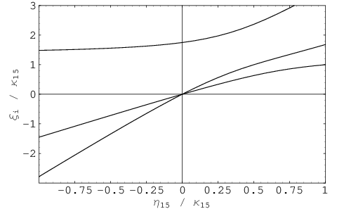
    so that their eigenvalues are identical. One of the four eigenvalues is always zero while, in general, the other three eigenvalues xix_{i} are non-vanishing. They can be determined as the solutions to the following cubic polynomial

    4​ξi3−ξi2​(18​η𝟏𝟓+7​κ𝟏𝟓−2​ρ𝟏𝟓+12​τ𝟏𝟓)\displaystyle 4\xi_{i}^{3}-\xi_{i}^{2}\left(18\eta_{\bf 15}+7\kappa_{\bf 15}-2\rho_{\bf 15}+12\tau_{\bf 15}\right)
    +ξi​(18​η𝟏𝟓2+27​η𝟏𝟓​κ𝟏𝟓−18​η𝟏𝟓​ρ𝟏𝟓−5​ρ𝟏𝟓2+36​η𝟏𝟓​τ𝟏𝟓+20​κ𝟏𝟓​τ𝟏𝟓)\displaystyle+\xi_{i}\left(18\eta_{\bf 15}^{2}+27\eta_{\bf 15}\kappa_{\bf 15}-18\eta_{\bf 15}\rho_{\bf 15}-5\rho_{\bf 15}^{2}+36\eta_{\bf 15}\tau_{\bf 15}+20\kappa_{\bf 15}\tau_{\bf 15}\right)
    −3​(8​η𝟏𝟓2​κ𝟏𝟓−8​η𝟏𝟓2​ρ𝟏𝟓−3​η𝟏𝟓​ρ𝟏𝟓2+8​η𝟏𝟓2​τ𝟏𝟓+12​η𝟏𝟓​κ𝟏𝟓​τ𝟏𝟓)=0,\displaystyle-3\left(8\eta_{\bf 15}^{2}\kappa_{\bf 15}-8\eta_{\bf 15}^{2}\rho_{\bf 15}-3\eta_{\bf 15}\rho_{\bf 15}^{2}+8\eta_{\bf 15}^{2}\tau_{\bf 15}+12\eta_{\bf 15}\kappa_{\bf 15}\tau_{\bf 15}\right)~=~0\ ,~~~~~~ (5.23)

    where ξi=F𝟏𝟓′m𝟏𝟓2​xi\xi_{i}=\frac{F^{\prime}_{\bf 15}}{m^{2}_{\bf 15}}x_{i}. Note that ξi\xi_{i} and xix_{i} have identical signs. To present a scenario in which all non-vanishing eigenvalues of the Hessian are positive let us again consider the special case with λ𝟏𝟓=ρ𝟏𝟓=τ𝟏𝟓=0\lambda_{\bf 15}=\rho_{\bf 15}=\tau_{\bf 15}=0. The condition 0<F𝟏𝟓′0<F^{\prime}_{\bf 15} as well as Eq. (5.21) demand positive κ𝟏𝟓\kappa_{\bf 15} in that case. With these assumptions the cubic polynomial simplifies and we can calculate the three roots. However, as the analytic expressions are rather lengthy, we show the results graphically in Figure 1. In order to have a minimum all three eigenvalues must be positive. This immediately implies positive η𝟏𝟓\eta_{\bf 15}. So in the case where λ𝟏𝟓=ρ𝟏𝟓=τ𝟏𝟓=0\lambda_{\bf 15}=\rho_{\bf 15}=\tau_{\bf 15}=0, the conditions to get a VEV that breaks S​U​(3)SU(3) down to 𝒵7⋊𝒵3\mathcal{Z}_{7}\rtimes\mathcal{Z}_{3} are

    0<κ𝟏𝟓,0<η𝟏𝟓.0\,<\,\kappa_{\bf 15}\ ,\quad 0\,<\,\eta_{\bf 15}\ . (5.24)
    Refer to caption
    Figure 1: 𝒵7⋊𝒵3\mathcal{Z}_{7}\rtimes\mathcal{Z}_{3} from the 𝟏𝟓{\bf 15} of S​U​(3)SU(3): the three non-vanishing scaled eigenvalues ξiκ𝟏𝟓\frac{\xi_{i}}{\kappa_{\bf 15}} of the sub-Hessian h4×4h_{4\times 4} are shown as functions of η𝟏𝟓κ𝟏𝟓\frac{\eta_{\bf 15}}{\kappa_{\bf 15}} in the case where λ𝟏𝟓=ρ𝟏𝟓=τ𝟏𝟓=0\lambda_{\bf 15}=\rho_{\bf 15}=\tau_{\bf 15}=0.

5.2 The case of a single 𝟏𝟎\boldsymbol{10}

Similar to the previous case, we consider a potential of a single 𝟏𝟎{\bf 10} which has a mass term 𝟏𝟎×𝟏𝟎¯{\bf 10\times\overline{10}} as well as quartic interactions of type 𝟏𝟎×𝟏𝟎×𝟏𝟎¯×𝟏𝟎¯{\bf 10\times 10\times\overline{10}\times\overline{10}}. The symmetric product

(𝟏𝟎×𝟏𝟎)s= 27+𝟐𝟖,({\bf 10\times 10})_{s}\,=\,{\bf 27+28}\ , (5.25)

shows that we can only write down two independent quartic S​U​(3)SU(3) invariants. Hence, the potential for the 𝟏𝟎{\bf 10} takes the form

V𝟏𝟎=−m𝟏𝟎2​ℐ𝟏𝟎(0)+λ𝟏𝟎​ℐ𝟏𝟎(1)+κ𝟏𝟎​ℐ𝟏𝟎(2),V_{\bf 10}~=~-m^{2}_{\bf 10}\,\mathcal{I}^{(0)}_{\bf 10}+\lambda_{\bf 10}\,\mathcal{I}^{(1)}_{\bf 10}+\kappa_{\bf 10}\,\mathcal{I}^{(2)}_{\bf 10}\ , (5.26)

with

ℐ𝟏𝟎(0)\displaystyle\mathcal{I}^{(0)}_{\bf 10} =\displaystyle= Ti​j​k​T¯i​j​k,\displaystyle T_{ijk}\>\overline{T}^{ijk}\ , (5.27)
ℐ𝟏𝟎(1)\displaystyle\mathcal{I}^{(1)}_{\bf 10} =\displaystyle= Ti​j​k​T¯i​j​k​Tl​m​n​T¯l​m​n,\displaystyle T_{ijk}\>\overline{T}^{ijk}~T_{lmn}\>\overline{T}^{lmn}\ , (5.28)
ℐ𝟏𝟎(2)\displaystyle\mathcal{I}^{(2)}_{\bf 10} =\displaystyle= Ti​j​m​T¯i​j​n​Tk​l​n​T¯k​l​m.\displaystyle T_{ijm}\>\overline{T}^{ijn}~T_{kln}\>\overline{T}^{klm}\ . (5.29)

Using the VEV configuration of Eq. (3.11) which breaks S​U​(3)SU(3) uniquely down to Δ⁡(27)\Delta(27), we can determine the scale of the VEV alignment by setting the first derivatives to zero. We obtain

|⟨ψ⟩|=m𝟏𝟎22​F𝟏𝟎⋅(1,1,1,0,0,0,0,0,0,0)T,|\langle\psi\rangle|~=~\sqrt{\frac{m^{2}_{\bf 10}}{2\,F_{\bf 10}}}\cdot(1,1,1,0,0,0,0,0,0,0)^{T}\ , (5.30)

with

F𝟏𝟎=3​λ𝟏𝟎+κ𝟏𝟎.F_{\bf 10}~=~3\,\lambda_{\bf 10}+\kappa_{\bf 10}\ . (5.31)

Having a minimum requires positive values for m𝟏𝟎2m^{2}_{\bf 10} and F𝟏𝟎F_{\bf 10}. The other constraints on the parameters of the potential arise from the Hessian. The 20×2020\times 20 matrix can be calculated analytically, yielding eleven zero eigenvalues as well as

4​m𝟏𝟎2,6×4​m𝟏𝟎2​κ𝟏𝟎3​F𝟏𝟎,and​2×4​m𝟏𝟎2​κ𝟏𝟎F𝟏𝟎.4m_{\bf 10}^{2}\ ,~~~~6~\times~\frac{4m_{\bf 10}^{2}\kappa_{\bf 10}}{3F_{\bf 10}}\ ,~~~\mathrm{and}~~~2~\times~\frac{4m_{\bf 10}^{2}\kappa_{\bf 10}}{F_{\bf 10}}\ . (5.32)

Consequently, we need positive κ𝟏𝟎\kappa_{\bf 10} in order to have a potential which is minimized by the VEV alignment of Eq. (3.11). The number of zero eigenvalues of the Hessian can be understood as follows. Eight zeros are due to the eight broken generators of S​U​(3)SU(3); another zero eigenvalues arises because the VEV also breaks a global U⁡(1)U(1). The remaining two vanishing eigenvalues are related to the existence of the second Δ⁡(27)\Delta(27) singlet within the 𝟏𝟎{\bf 10}. Any linear combination of the VEV alignments in Eq. (3.10) and Eq. (3.11) leaves the group Δ⁡(27)\Delta(27) intact. Hence, the additional two zero eigenvalues of the Hessian correspond to the directions of the real and the imaginary part of ψ10\psi_{10}. Sliding along this direction, the residual symmetry will remain Δ⁡(27)\Delta(27) as long as ⟨ψ1,2,3⟩≠0\langle\psi_{1,2,3}\rangle\neq 0. Only in the special vacuum where the first three components of the 𝟏𝟎{\bf 10} vanish identically, we end up with the bigger group given in Eq. (4.8). This can be avoided by small deformations of the potential. A simple scenario could consist in adding a second 𝟏𝟎{\bf 10} which is aligned as in Eq. (3.10), cf. section 5.3. We can then introduce a quartic term which couples the two different 𝟏𝟎{\bf 10}s as follows,

∑a,b=110(ψa​ψa′¯)​(ψb¯​ψb′).\sum_{a,b=1}^{10}(\psi_{a}\,\overline{\psi_{a}^{\prime}})\,(\overline{\psi_{b}}\,\psi^{\prime}_{b})\ . (5.33)

Note that such a term is always positive or zero. Assuming this term to enter the potential with a positive coupling constant, the minimum arises if ∑a=110⟨ψa⟩​⟨ψa′¯⟩=0\sum_{a=1}^{10}\langle\psi_{a}\rangle\,\langle\overline{\psi_{a}^{\prime}}\rangle=0. With ⟨ψa′⟩=0\langle\psi^{\prime}_{a}\rangle=~\!\!0 for a=1,2,…,9a=1,2,...,9, this entails vanishing ⟨ψ10⟩\langle\psi_{10}\rangle. Therefore, the VEV of ψ\psi is driven to the alignment of Eq. (3.11) which breaks S​U​(3)SU(3) uniquely down to Δ⁡(27)\Delta(27).

5.3 The case of a 𝟏𝟎\boldsymbol{10} and a 𝟔\boldsymbol{6}

We have seen in section 4 that the combination of a 𝟔{\bf 6} and a 𝟏𝟎{\bf 10} with alignments along the directions of Eqs. (3.9,3.10) gives rise to a residual 𝒜4\mathcal{A}_{4} symmetry. In the following we show that there exists a potential which assumes its minimum for exactly these VEV alignments. The most general renormalizable potential of one 𝟔{\bf 6} and one 𝟏𝟎{\bf 10} consists of thirteen invariants. It reads

V𝟔+𝟏𝟎\displaystyle V_{\bf 6+10} =\displaystyle= −m𝟔2​ℐ𝟔(0)+λ𝟔​ℐ𝟔(1)+κ𝟔​ℐ𝟔(2)+ρ𝟔​ℐ𝟔(3)\displaystyle-m^{2}_{\bf 6}\,\mathcal{I}^{(0)}_{\bf 6}+\lambda_{\bf 6}\,\mathcal{I}^{(1)}_{\bf 6}+\kappa_{\bf 6}\,\mathcal{I}^{(2)}_{\bf 6}+\rho_{\bf 6}\,\mathcal{I}^{(3)}_{\bf 6} (5.34)
−m𝟏𝟎2​ℐ𝟏𝟎(0)+λ𝟏𝟎​ℐ𝟏𝟎(1)+κ𝟏𝟎​ℐ𝟏𝟎(2)+ρ𝟏𝟎​ℐ𝟏𝟎(3)+τ𝟏𝟎​ℐ𝟏𝟎(4)\displaystyle-m^{2}_{\bf 10}\,\mathcal{I}^{(0)}_{\bf 10}+\lambda_{\bf 10}\,\mathcal{I}^{(1)}_{\bf 10}+\kappa_{\bf 10}\,\mathcal{I}^{(2)}_{\bf 10}+\rho_{\bf 10}\,\mathcal{I}^{(3)}_{\bf 10}+\tau_{\bf 10}\,\mathcal{I}^{(4)}_{\bf 10}
+η1​ℐ𝟔+𝟏𝟎(1)+η2​ℐ𝟔+𝟏𝟎(2)+η3​ℐ𝟔+𝟏𝟎(3)+η4​ℐ𝟔+𝟏𝟎(4),\displaystyle+\,\eta_{1}\,\mathcal{I}^{(1)}_{\bf 6+10}+\eta_{2}\,\mathcal{I}^{(2)}_{\bf 6+10}+\eta_{3}\,\mathcal{I}^{(3)}_{\bf 6+10}+\eta_{4}\,\mathcal{I}^{(4)}_{\bf 6+10}\ ,

with

ℐ𝟔(0)\displaystyle\mathcal{I}^{(0)}_{\bf 6} =\displaystyle= Ti​j​T¯i​j,\displaystyle T_{ij}\>\overline{T}^{ij}\ , (5.35)
ℐ𝟔(1)\displaystyle\mathcal{I}^{(1)}_{\bf 6} =\displaystyle= Ti​j​T¯i​j​Tk​l​T¯k​l,\displaystyle T_{ij}\>\overline{T}^{ij}~T_{kl}\>\overline{T}^{kl}\ , (5.36)
ℐ𝟔(2)\displaystyle\mathcal{I}^{(2)}_{\bf 6} =\displaystyle= Ti​k​T¯i​l​Tj​l​T¯j​k,\displaystyle T_{ik}\>\overline{T}^{il}~T_{jl}\>\overline{T}^{jk}\ , (5.37)
ℐ𝟔(3)\displaystyle\mathcal{I}^{(3)}_{\bf 6} =\displaystyle= ϵi​j​k​T1​i​T2​j​T3​k+h.c.,\displaystyle\epsilon^{ijk}\,T_{1i}\>{T}_{2j}\>T_{3k}~+~\mathrm{h.c.}\ , (5.38)
ℐ𝟏𝟎(3)\displaystyle\mathcal{I}^{(3)}_{\bf 10} =\displaystyle= ϵx​x′​k​ϵy​y′​l​Ti​x​y​Tj​x′​y′​Tm​k​l​T¯i​j​m+h.c.,\displaystyle\epsilon^{xx^{\prime}k}\epsilon^{yy^{\prime}l}\,T_{ixy}\>T_{jx^{\prime}y^{\prime}}~T_{mkl}\>\overline{T}^{ijm}~+~\mathrm{h.c.}\ , (5.39)
ℐ𝟏𝟎(4)\displaystyle\mathcal{I}^{(4)}_{\bf 10} =\displaystyle= ϵx​x′​k​ϵy​y′​l​Ti​x​y​Tj​x′​y′​ϵv​v′​i​ϵw​w′​j​Tk​v​w​Tl​v′​w′+h.c.,\displaystyle\epsilon^{xx^{\prime}k}\epsilon^{yy^{\prime}l}\,T_{ixy}\>T_{jx^{\prime}y^{\prime}}~\epsilon^{vv^{\prime}i}\epsilon^{ww^{\prime}j}\,T_{kvw}\>T_{lv^{\prime}w^{\prime}}~+~\mathrm{h.c.}\ , (5.40)
ℐ𝟔+𝟏𝟎(1)\displaystyle\mathcal{I}^{(1)}_{\bf 6+10} =\displaystyle= Ti​j​T¯i​j​Tk​l​m​T¯k​l​m,\displaystyle T_{ij}\>\overline{T}^{ij}~T_{klm}\>\overline{T}^{klm}\ , (5.41)
ℐ𝟔+𝟏𝟎(2)\displaystyle\mathcal{I}^{(2)}_{\bf 6+10} =\displaystyle= Ti​j​m​T¯i​j​Tk​l​T¯k​l​m,\displaystyle T_{ijm}\>\overline{T}^{ij}~T_{kl}\>\overline{T}^{klm}\ , (5.42)
ℐ𝟔+𝟏𝟎(3)\displaystyle\mathcal{I}^{(3)}_{\bf 6+10} =\displaystyle= Ti​j​m​T¯i​j​n​Tk​n​T¯k​m,\displaystyle T_{ijm}\>\overline{T}^{ijn}~T_{kn}\>\overline{T}^{km}\ , (5.43)
ℐ𝟔+𝟏𝟎(4)\displaystyle\mathcal{I}^{(4)}_{\bf 6+10} =\displaystyle= ϵx​x′​k​ϵy​y′​l​Ti​x​y​Tj​x′​y′​Tk​l​T¯i​j+h.c.,\displaystyle\epsilon^{xx^{\prime}k}\epsilon^{yy^{\prime}l}\,T_{ixy}\>T_{jx^{\prime}y^{\prime}}~T_{kl}\>\overline{T}^{ij}~+~\mathrm{h.c.}\ , (5.44)

and ℐ𝟏𝟎(0)\mathcal{I}^{(0)}_{\bf 10}, ℐ𝟏𝟎(1)\mathcal{I}^{(1)}_{\bf 10}, ℐ𝟏𝟎(2)\mathcal{I}^{(2)}_{\bf 10} as given in Eqs. (5.27-5.29). The tensors T...T_{...} with three indices correspond to the 𝟏𝟎{\bf 10} while those with two indices stand for the 𝟔{\bf 6}; a bar indicates complex conjugate representations. ϵi​j​k\epsilon^{ijk} denotes the totally antisymmetric tensor with ϵ123=1\epsilon^{123}=1. Note that all invariants which contain this ϵ\epsilon tensor are not symmetric under a general U⁡(1)U(1) while all other invariants feature such a U⁡(1)U(1) symmetry.

Evaluation of the first derivatives using the alignment directions of Eqs. (3.9,3.10) fixes the scale of the VEVs,

⟨χ⟩=R𝟔​(1,1,1,0,0,0)T,⟨ψ⟩=R𝟏𝟎​(0,0,0,0,0,0,0,0,0,1)T.\displaystyle\langle\chi\rangle\,=\,R_{\bf 6}\,(1,1,1,0,0,0)^{T}\ ,\qquad\langle\psi\rangle\,=\,R_{\bf 10}\,(0,0,0,0,0,0,0,0,0,1)^{T}\ . (5.45)

Despite the lack of a general U⁡(1)U(1) symmetry we can assume real VEVs R𝟔R_{\bf 6} and R𝟏𝟎R_{\bf 10} for our purposes, because any potential V′V^{\prime} which is minimized by complex VEVs corresponds to a modified potential VV in which the coupling constants absorb the phases of the complex VEVs, thus rendering the latter real. With this assumption we obtain the following two conditions on R𝟔R_{\bf 6} and R𝟏𝟎R_{\bf 10},

0\displaystyle 0 =\displaystyle= −3​m𝟔2+R𝟏𝟎2​(3​η1+η3−2​η4)+3​R𝟔​(6​R𝟔​λ𝟔+2​R𝟔​κ𝟔+ρ𝟔),\displaystyle-3m_{\bf 6}^{2}+R_{\bf 10}^{2}(3\eta_{1}+\eta_{3}-2\eta_{4})+3R_{\bf 6}(6R_{\bf 6}\lambda_{\bf 6}+2R_{\bf 6}\kappa_{\bf 6}+\rho_{\bf 6})\ ,
0\displaystyle 0 =\displaystyle= −3​m𝟏𝟎2+3​R𝟔2​(3​η1+η3−2​η4)+2​R𝟏𝟎2​(3​λ𝟏𝟎+κ𝟏𝟎+2​ρ𝟏𝟎+4​τ𝟏𝟎).\displaystyle-3m_{\bf 10}^{2}+3R_{\bf 6}^{2}(3\eta_{1}+\eta_{3}-2\eta_{4})+2R_{\bf 10}^{2}(3\lambda_{\bf 10}+\kappa_{\bf 10}+2\rho_{\bf 10}+4\tau_{\bf 10})\ .

For the sake of simplicity we assume ρ𝟔=0\rho_{\bf 6}=0.55 5 This could be enforced by a U⁡(1)U(1) symmetry under which the 𝟔{\bf 6} carries non-vanishing charge while the 𝟏𝟎{\bf 10} is neutral. Then the above conditions are satisfied for

R𝟔2\displaystyle R_{\bf 6}^{2} =\displaystyle= 2​m𝟔2​(3​λ𝟏𝟎+κ𝟏𝟎+2​ρ𝟏𝟎+4​τ𝟏𝟎)−m𝟏𝟎2​(3​η1+η3−2​η4)4​(3​λ𝟔+κ𝟔)​(3​λ𝟏𝟎+κ𝟏𝟎+2​ρ𝟏𝟎+4​τ𝟏𝟎)−(3​η1+η3−2​η4)2,\displaystyle\frac{2m_{\bf 6}^{2}(3\lambda_{\bf 10}+\kappa_{\bf 10}+2\rho_{\bf 10}+4\tau_{\bf 10})-m_{\bf 10}^{2}(3\eta_{1}+\eta_{3}-2\eta_{4})}{4(3\lambda_{\bf 6}+\kappa_{\bf 6})(3\lambda_{\bf 10}+\kappa_{\bf 10}+2\rho_{\bf 10}+4\tau_{\bf 10})-(3\eta_{1}+\eta_{3}-2\eta_{4})^{2}}\ , (5.46)
R𝟏𝟎2\displaystyle R_{\bf 10}^{2} =\displaystyle= 6​m𝟏𝟎2​(3​λ𝟔+κ𝟔)−3​m𝟔2​(3​η1+η3−2​η4)4​(3​λ𝟔+κ𝟔)​(3​λ𝟏𝟎+κ𝟏𝟎+2​ρ𝟏𝟎+4​τ𝟏𝟎)−(3​η1+η3−2​η4)2.\displaystyle\frac{6m_{\bf 10}^{2}(3\lambda_{\bf 6}+\kappa_{\bf 6})-3m_{\bf 6}^{2}(3\eta_{1}+\eta_{3}-2\eta_{4})}{4(3\lambda_{\bf 6}+\kappa_{\bf 6})(3\lambda_{\bf 10}+\kappa_{\bf 10}+2\rho_{\bf 10}+4\tau_{\bf 10})-(3\eta_{1}+\eta_{3}-2\eta_{4})^{2}}\ . (5.47)

Evaluating the second derivatives for these VEVs yields a block diagonal structure for the 32×3232\times 32 Hessian

H=h1×1⊕h4×4⊕3×h4×4′⊕3×h4×4′′⊕03×3.H~=~h_{1\times 1}~\oplus~h_{4\times 4}~\oplus~3\times h_{4\times 4}^{\prime}~\oplus~3\times h_{4\times 4}^{\prime\prime}~\oplus~0_{3\times 3}\ . (5.48)

In general, h1×1h_{1\times 1} and h4×4h_{4\times 4} have no vanishing eigenvalue, while h4×4′h_{4\times 4}^{\prime} and h4×4′′h_{4\times 4}^{\prime\prime} each have one zero eigenvalue. Therefore the full Hessian exhibits nine zero eigenvalues corresponding to the directions of the eight S​U​(3)SU(3) transformations plus an extra U⁡(1)U(1) transformation. Notice that there exists only one U⁡(1)U(1) symmetry and not two because the charge of the 𝟏𝟎{\bf 10} is fixed to be neutral. In order to have a minimum we need the remaining 23 eigenvalues to be positive. This constrains the set of parameters of the potential V𝟔+𝟏𝟎V_{\bf 6+10} in Eq. (5.34). As an example we discuss the special case where

m𝟔=m𝟏𝟎=m,κ𝟔=κ𝟏𝟎=κ,η4=η,m_{\bf 6}=m_{\bf 10}=m\ ,\qquad\kappa_{\bf 6}=\kappa_{\bf 10}=\kappa\ ,\qquad\eta_{4}=\eta\ , (5.49)
λ𝟔=λ𝟏𝟎=ρ𝟔=ρ𝟏𝟎=τ𝟏𝟎=η1=η2=η3=0.\lambda_{\bf 6}=\lambda_{\bf 10}=\rho_{\bf 6}=\rho_{\bf 10}=\tau_{\bf 10}=\eta_{1}=\eta_{2}=\eta_{3}=0\ . (5.50)

Then the VEVs simplify to

R𝟔2=m22​(κ−η),R𝟏𝟎2=3​m22​(κ−η),R_{\bf 6}^{2}=\frac{m^{2}}{2(\kappa-\eta)}\ ,\qquad R_{\bf 10}^{2}=\frac{3m^{2}}{2(\kappa-\eta)}\ , (5.51)

requiring positive m2m^{2} as well as η<κ\eta<\kappa. The eigenvalues of the sub-Hessians are calculated to be

h1×1:\displaystyle h_{1\times 1}: 4​m2​ηκ−η,\displaystyle\frac{4m^{2}\eta}{\kappa-\eta}\ , (5.52)
h4×4:\displaystyle h_{4\times 4}: 4​m2,4​m2​(κ+η)κ−η2×4​m2​κκ−η,\displaystyle 4m^{2}\ ,\qquad\frac{4m^{2}(\kappa+\eta)}{\kappa-\eta}\qquad 2~\times~\frac{4m^{2}\kappa}{\kappa-\eta}\ , (5.53)
h4×4′:\displaystyle h_{4\times 4}^{\prime}: x1,x2,x3,0,\displaystyle x_{1}\ ,\quad x_{2}\ ,\quad x_{3}\ ,\quad 0\ , (5.54)
h4×4′′:\displaystyle h_{4\times 4}^{\prime\prime}: 4​m2​(2​κ+3​η)3​(κ−η),m2​η​(13±109)3​(κ−η),0,\displaystyle\frac{4m^{2}(2\kappa+3\eta)}{3(\kappa-\eta)}\ ,\qquad\frac{m^{2}\eta(13\pm\sqrt{109})}{3(\kappa-\eta)}\ ,\qquad 0\ , (5.55)

where xix_{i} are the solutions to the cubic polynomial

3​ξi3​(η−κ)3+2​ξi2​(η−κ)2​(11​η+10​κ)\displaystyle 3\xi_{i}^{3}(\eta-\kappa)^{3}+2\xi^{2}_{i}(\eta-\kappa)^{2}(11\eta+10\kappa)
+4​ξi​(η−κ)​(7​η2+22​η​κ+8​κ2)−16​η​(η2−2​η​κ−4​κ2)=0,\displaystyle+4\xi_{i}(\eta-\kappa)(7\eta^{2}+22\eta\kappa+8\kappa^{2})-16\eta(\eta^{2}-2\eta\kappa-4\kappa^{2})~=~0\ ,~~~~~~~ (5.56)

with ξi=xim2\xi_{i}=\frac{x_{i}}{m^{2}}. Figure 2 presents the results graphically for the relevant region

0<η<κ,0\,<\,\eta\,<\,\kappa\ , (5.57)

which is obtained from requiring positive values for the other eigenvalues of the Hessian. From this example it is clear that parameter ranges exist in which the potential V𝟔+𝟏𝟎V_{\bf 6+10} of Eq. (5.34) is minimized by the alignments of Eqs. (3.9,3.10). Hence 𝒜4\mathcal{A}_{4} can result as the discrete remnant of a spontaneously broken S​U​(3)SU(3) symmetry.

Refer to caption
Figure 2: 𝒜4\mathcal{A}_{4} from a 𝟔{\bf 6} and a 𝟏𝟎{\bf 10} of S​U​(3)SU(3): the three non-vanishing scaled eigenvalues ξi\xi_{i} of the sub-Hessian h4×4′h_{4\times 4}^{\prime} are shown as functions of ηκ\frac{\eta}{\kappa} in the special case of Eqs. (5.49,5.50).

6 Conclusion

In this paper we have investigated the possibility of obtaining a non-Abelian discrete family symmetry 𝒢\mathcal{G} from an underlying S​U​(3)SU(3) gauge symmetry. Such a scenario is appealing in the sense that the residual discrete symmetry is protected against violations by quantum gravity effects. We have first identified the higher S​U​(3)SU(3) representations which contain singlets under various discrete subgroups. These are potential candidates of fields that are capable of breaking S​U​(3)SU(3) down to 𝒢\mathcal{G}. Fixing the basis of the subgroup, we have determined the 𝒢\mathcal{G} singlet directions and checked whether these vacuum alignments leave invariant the desired subgroups or something bigger. Scrutinizing various S​U​(3)SU(3) invariant potentials which involve higher representations comprises the central part of the paper. Constraining ourselves to the irreps 𝟔{\bf 6}, 𝟏𝟎{\bf 10} and 𝟏𝟓{\bf 15} we found that 𝒜4\mathcal{A}_{4}, undoubtedly the most popular family symmetry, can be generated from either a single 𝟏𝟓{\bf 15} or alternatively a combination of a 𝟔{\bf 6} and a 𝟏𝟎{\bf 10}. Similarly, the group 𝒵7⋊𝒵3\mathcal{Z}_{7}\rtimes\mathcal{Z}_{3} is obtained from a single 𝟏𝟓{\bf 15}, however using different numerical values for the coupling constants of the potential. Finally, a single 𝟏𝟎{\bf 10} allows to break S​U​(3)SU(3) down to the group Δ⁡(27)\Delta(27). These results show that an S​U​(3)SU(3) gauge symmetry can give rise to non-Abelian discrete family symmetries, sometimes adopting only one S​U​(3)SU(3) breaking multiplet. Having discussed the above examples in great detail, it should be clear how to proceed in the case of other discrete symmetries 𝒢\mathcal{G}. For instance, the family symmetry 𝒫​𝒮​ℒ2​(7)\mathcal{PSL}_{2}(7) is expected to arise from an appropriate vacuum alignment of the 𝟏𝟓′{\bf 15^{\prime}} of S​U​(3)SU(3). This case will be treated elsewhere. In the context of a concrete model [29] we hope to find a solution to an unexplained tuning which is required to generate the correct vacuum structure of the flavon sextets.

We conclude by pointing out that our work does not address the question of how the breaking of the continuous symmetry is communicated to the Yukawa sector. In general this is a very model dependent problem as there are different choices for assigning the Standard Model fermions as well as the 𝒢\mathcal{G} breaking flavons to irreps of the underlying S​U​(3)SU(3) symmetry. Depending on this choice the product rules constrain the allowed interactions of the S​U​(3)SU(3) breaking field(s) to the chiral fermions and flavons. Such an investigation should be carried out within the context of a specific flavor model and is therefore beyond the scope of our paper.

Acknowledgments

I am indebted to Pierre Ramond and Steve King for encouragement and stimulating discussions. I wish to specially thank Pierre Ramond for reading the manuscript and his helpful comments. This work is supported by the STFC Rolling Grant ST/G000557/1.

References

  • [1] T. Schwetz, M. A. Tórtola and J. W. F. Valle, New J. Phys. 10 (2008) 113011 [arXiv:0808.2016].
  • [2] M. C. Gonzalez-Garcia, M. Maltoni and J. Salvado, JHEP 1004 (2010) 056 [arXiv:1001.4524].
  • [3] P. F. Harrison, D. H. Perkins and W. G. Scott, Phys. Lett. B 530 (2002) 167 [hep-ph/0202074].
  • [4] P. F. Harrison and W. G. Scott, Phys. Lett. B 535 (2002) 163 [hep-ph/0203209].
  • [5] G. Altarelli and F. Feruglio, Rev. Mod. Phys. 82 (2010) 2701 [arXiv:1002.0211].
  • [6] L. M. Krauss and F. Wilczek, Phys. Rev. Lett. 62 (1989) 1221.
  • [7] L. E. Ibáñez and G. G. Ross, Phys. Lett. B 260 (1991) 291.
  • [8] L. E. Ibáñez and G. G. Ross, Nucl. Phys. B 368 (1992) 3.
  • [9] H. K. Dreiner, C. Luhn and M. Thormeier, Phys. Rev. D 73 (2006) 075007 [hep-ph/0512163].
  • [10] C. Luhn and M. Thormeier, Phys. Rev. D 77 (2008) 056002 [arXiv:0711.0756].
  • [11] B. A. Ovrut, J. Math. Phys. 19 (1978) 418.
  • [12] G. Etesi, J. Math. Phys. 37 (1996) 1596 [hep-th/9706029].
  • [13] M. Koca, M. Al-Barwani and R. Koc, J. Phys. A 30 (1997) 2109.
  • [14] M. Koca, R. Koc and H. Tutunculer, Int. J. Mod. Phys. A 18 (2003) 4817 [hep-ph/0410270].
  • [15] J. Berger and Y. Grossman, JHEP 1002 (2010) 071 [arXiv:0910.4392].
  • [16] A. Adulpravitchai, A. Blum and M. Lindner, JHEP 0909 (2009) 018 [arXiv:0907.2332].
  • [17] C. Luhn and P. Ramond, JHEP 0807 (2008) 085 [arXiv:0805.1736].
  • [18] G. A. Miller, H. F. Blichfeldt, and L. E. Dickson, Theory and application of finite groups, John Wiley & Sons, New York (1916), and Dover edition (1961).
  • [19] W. M. Fairbairn, T. Fulton, W. H. Klink, J. Math. Phys. 5 (1964) 1038.
  • [20] A. Bovier, M. Lüling, and D. Wyler, J. Math. Phys. 22 (1981) 1543.
  • [21] C. Luhn, S. Nasri and P. Ramond, J. Math. Phys. 48 (2007) 073501 [hep-th/0701188].
  • [22] C. Luhn, S. Nasri and P. Ramond, J. Math. Phys. 48 (2007) 123519 [arXiv:0709.1447].
  • [23] J. A. Escobar and C. Luhn, J. Math. Phys. 50 (2009) 013524 [arXiv:0809.0639].
  • [24] P. O. Ludl, arXiv:0907.5587.
  • [25] H. Ishimori, T. Kobayashi, H. Ohki, H. Okada, Y. Shimizu and M. Tanimoto, Prog. Theor. Phys. Suppl. 183 (2010) 1 [arXiv:1003.3552].
  • [26] W. Grimus and P. O. Ludl, J. Phys. A 43 (2010) 445209 [arXiv:1006.0098].
  • [27] P. Ramond, Group theory: a physicist’s survey, Cambridge University Press, Cambridge, UK (2010).
  • [28] S. F. King and C. Luhn, JHEP 0910 (2009) 093 [arXiv:0908.1897].
  • [29] S. F. King and C. Luhn, Nucl. Phys. B 832 (2010) 414 [arXiv:0912.1344].