Minimum Covering with Travel CostThanks: A preliminary extended abstract of this paper appears in [11]. A 4-page abstract based on Sections 3 and 4 of this paper appeared in the informal and non-selective workshop “EuroCG”, March 2009 [13].
Abstract
Given a polygon and a visibility range, the Myopic Watchman Problem with Discrete Vision (MWPDV) asks for a closed path and a set of scan points , such that (i) every point of the polygon is within visibility range of a scan point; and (ii) path length plus weighted sum of scan number along the tour is minimized. Alternatively, the bicriteria problem (ii’) aims at minimizing both scan number and tour length. We consider both lawn mowing (in which tour and scan points may leave ) and milling (in which tour, scan points and visibility must stay within ) variants for the MWPDV; even for simple special cases, these problems are NP-hard.
We show that this problem is NP-hard, even for the special cases of rectilinear polygons and scan range 1, and negligible small travel cost or negligible travel cost. For rectilinear MWPDV milling in grid polygons we present a 2.5-approximation with unit scan range; this holds for the bicriteria version, thus for any linear combination of travel cost and scan cost. For grid polygons and circular unit scan range, we describe a bicriteria 4-approximation. These results serve as stepping stones for the general case of circular scans with scan radius and arbitrary polygons of feature size , for which we extend the underlying ideas to a bicriteria approximation algorithm. Finally, we describe approximation schemes for MWPDV lawn mowing and milling of grid polygons, for fixed ratio between scan cost and travel cost.
Keywords: Covering, Minimum Watchman Problem, limited visibility, lawn mowing, bicriteria problems, approximation algorithm, PTAS.
1 Introduction
Covering a given polygonal region by a small set of disks or squares is a problem with many applications. Another classical problem is finding a short tour that visits a number of objects. Both of these aspects have been studied separately, with generalizations motivated by natural constraints.
In this paper, we study the combination of these problems, originally motivated by challenges from robotics, where accurate scanning requires a certain amount of time for each scan; obviously, this is also the case for other surveillance tasks that combine changes of venue with stationary scanning. The crucial constraints are (a) a limited visibility range, and (b) the requirement to stop when scanning the environment, i.e., with vision only at discrete points. These constraints give rise to the Myopic Watchman Problem with Discrete Vision (MWPDV), the subject of this paper.
For a scan range that is not much bigger than the feature size of the polygon, the MWPDV combines two geometric problems that allow approximation schemes (minimum cover and TSP). This makes it tempting to assume that combining two approximation schemes will yield a polynomial-time approximation scheme (PTAS), e.g., by using a PTAS for minimum cover (Hochbaum and Maass [15]), then a PTAS for computing a tour on this solution. As can be seen from Figure 1(a) and (b), this is not the case; moreover, an optimal solution depends on the relative weights of tour length and scan cost. This turns the task into a bicriteria problem; the example shows that there is no simultaneous PTAS for both aspects. As we will see in Sections 4 and 5, a different approach allows a simultaneous constant-factor approximation for both scan number and tour length, and thus of the combined cost. We show in Section 7, a more involved integrated guillotine approach allows a PTAS for combined cost in the case of a fixed ratio between scan cost and travel cost.

(a)

(b)

(c)
A different kind of difficulty is highlighted in Figure 1(c), where an example called “wells” ([2]) is illustrated: For a visibility range that is large compared to the size of the niches (the “wells”), it may be quite hard to determine a guard cover of small size, since it is not clear what should be a small set of candidate guard locations that suffice for coverage. Each “well” is covered by a pair of points, whose locations need not correspond, e.g., to vertices in the arrangement of visibility polygons of the vertices of the polygon. In fact, because of this difficulty, there is no known nontrivial (with factor ) approximation for minimum guard cover in simple -gons. With an assumption about a sufficient set of guard points (e.g., vertices of the polygon or a grid within the polygon), an -approximation by Efrat and Har-Peled [10] is known. Also note that the optimal solution for our problem may change significantly with the relative weights between tour length and scan cost: If the tour length dominates the number of scans in the objective function, an optimal tour can be forced to follow the row of niches on the right in the figure. We will show in Section 6 how to obtain a constant-factor approximation for a bounded value , being the minimum side length of .
Related Work. Closely related to practical problems of searching with an autonomous robot is the classical theoretical problem of finding a shortest watchman tour; e.g., see [7, 8]. Planning an optimal set of scan points (with unlimited visibility) is the art gallery problem [20]. Finally, visiting all grid points of a given set is a special case of the classical Traveling Salesman Problem (TSP); see [16]. Two generalizations of the TSP are the so-called lawn mowing and milling problems: Given a cutter of a certain shape, e.g., an axis-aligned square, the milling problem asks for a shortest tour along which the (center of the) cutter moves, such that the entire region is covered and the cutter stays inside the region at all times. Clearly, this takes care of the constraint of limited visibility, but it fails to account for discrete visibility. At this point, the best known approximation method for milling is a 2.5-approximation [3]. Related results for the TSP with neighborhoods (TSPN) include [9, 19]; further variations arise from considering online scenarios, either with limited vision [6] or with discrete vision [14, 12], but not both. The discrete visibility is intrinsic to the art gallery problem, but no tour is considered here. For this problem neither constant-factor approximation algorithms nor exact solution methods are known, recent results include an algorithm based on linear programming that provides lower bounds on the necessary number of guards in every step and—in case of convergence and integrality—ends with an optimal solution by Baumgartner et al. [4]. Finally, [1] consider covering a set of points by a number of scans, and touring all scan points, with the objective function being a linear combination of scan cost and travel cost; however, the set to be scanned is discrete, and scan cost is a function of the scan radius, which may be small or large.
For an online watchman problem with unrestricted but discrete vision, Fekete and Schmidt [14] present a comprehensive study of the milling problem, including a strategy with constant competitive ratio for polygons of bounded feature size and with the assumption that each edge of the polygon is fully visible from some scan point. For limited visibility range, Wagner et al. [23] discuss an online strategy that chooses an arbitrarily uncovered point on the boundary of the visibility circle and backtracks if no such point exists. For the cost they only consider the length of the path used between the scan points, scanning causes no cost. Then, they can give an upper bound on the cost as a ratio of total area to cover and squared radius.
Our Results. On the positive side, we give a 2.5-approximation for the case of grid polygons and a rectangular range of unit-range visibility, generalizing the 2.5-approximation by Arkin, Fekete, and Mitchell [3] for continuous milling. The underlying ideas form the basis for more general results: For circular scans of radius and grid polygons we give a 4-approximation. Moreover, for circular scans of radius and arbitrary polygons of feature size , we extend the underlying ideas to a -approximation algorithm. All these results also hold for the bicriteria versions, for which both scan cost and travel cost have to be approximated simultaneously. Finally, we present a PTAS for MWPDV lawn mowing and a PTAS for MWPDV milling, both for the case of fixed ratio between scan cost and travel cost.
The rest of the paper is organized as follows. In the following Section 2 we give the notation and formally define the Myopic Watchman Problem with Discrete Vision. Section 3 provides a NP-hardness proof. Approximation algorithms for grid polygons and rectangular unit scan range, grid polygons and circular unit scan range as well as for general polygons and circular scan range are presented in Sections 4, 5 and 6, respectively. A description of polynomial-time approximation schemes for both the lawn mowing and the milling variant are given in Section 7. In the final Section 8 we discuss possible implications and extensions.
2 Notation and Preliminaries
We are given a polygon . In general, may be a polygon with holes; in Sections 3, 4 and 5, is an axis-parallel polygon with integer coordinates.
Our robot, , has discrete vision, i.e., it can perceive its environment when it stops at a point and performs a scan, which takes time units. From a scan point , only a ball of radius is visible to , either in - or -metric. A set of scan points covers the polygon , if and only if for each point there exists a scan point such that sees (i.e., ) and .
We then define the Myopic Watchman Problem with Discrete Vision (MWPDV) as follows: Our goal is to find a tour and a set of scan points that covers , such that the total travel and scan time is optimal, i.e., we minimize , where is the length of tour . Alternatively, we may consider the bicriteria problem, and aim for a simultaneous approximation of both scan number and tour length.
3 NP-Hardness
Even the simplest and extreme variants of MWPDV lawn mowing are still generalizations of NP-hard problems.
Theorem 1.
- (1)
The MWPDV is NP-hard, even for polyominoes and small or no scan cost, i.e., or .
- (2)
The MWPDV is NP-hard, even for polyominoes and small travel cost, i.e., .
- (3)
The MWPDV is NP-hard, even for polyominoes and no travel cost, i.e., .
Proof.
The first claim is a result of the hardness of minimum cost milling, see [3]. The second claim is an easy consequence of the NP-hardness of Hamiltonicity of Grid Graphs (HGG) [16]: Given an instance of HGG with vertices, turn it into an instance of MWPDV by scaling the grid graph by a factor of two, and replacing each grid point of by a 2x2-square. This yields a canonical set of scan points that is contained in any optimal WMPDV tour; traveling these with a tour length is possible if and only the graph is Hamiltonian.
The third claim is closely related to a minimum cover problem by visibility discs; however, the MWPDV requires that the scan points must be inside of the polygonal region. We give a proof along the lines of [5], based on a reduction of the NP-hard problem Planar 3SAT, a special case of 3SAT in which the variable-clause incidence graph is planar. As a first step, we construct an appropriate planar layout of the graph , e.g., by using the method of Rosenstiehl and Tarjan [21]. This layout is turned into a grid polygon by representing the variables, the clauses and the edges of . An example for the variable component is given in Figure 2.


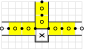
The variable gadgets allow two ways for locating a minimum number of scan points. The first (the black points in Figure 2) relates to a setting of “true”, the other (the circles in Figure 2) to a setting of “false”. For the variable setting “true” the scan squares are pushed further into the edge corridor. These edge corridors are similar to the variable-circles—bendings are done accordingly. In order to have the same number of points and circles, edge corridors may be added, that do not end in another polygonal piece, but assure this parity (with circles at the edge corridor).
A clause component is given in Figure 3. Edge corridors of the three associated variables (each with the appropriate truth setting) meet in the polygonal piece for the clause (dark gray in Figure 3). If and only if the clause is satisfied, i.e., if at least in one edge corridor a scan square is placed at a black point, three additional scans suffice to cover this polygonal piece. Otherwise, four scans are necessary.
Given the components defined above we can compute the parameter , the number of scan squares necessary to cover the entire resulting polygon . is polynomial in the number of vertices of and part of the input. All vertices of the resulting have integer coordinates of small size, their number is polynomial in the number of vertices of . This shows that the problem is NP-hard. ∎

(a)

(b)

(c)
∎
4 Approximating Rectilinear MWPDV Milling for Rectangular Visibility Range
As a first step (and a warmup for more general cases), we give an approximation algorithm for rectilinear visibility range in rectilinear grid polygons.
The following lemma allows us to focus on visiting and scanning at grid points.
Lemma 2.
For a rectilinear pixel polygon there exists an optimum myopic watchman tour such that all scan points are located on grid points:
| (1) |
Proof.
Let be an optimal tour, with scan points not located on grid points. Consider the vertical and horizontal strips of pixels in of maximal length. W.l.o.g., we start with the horizontal strips. For every strip, we shift the scans, such that the x-coordinates are integers (starting from the boundary, i.e., with distance to the boundary if possible, and away from non-reflex corners). The tour will not be longer, we cover not less; in case we are able to reduce the number of scans per strip by one we have a contradiction to being optimal. After applying this to all horizontal strips we proceed analogously for the vertical strips. Hence, we have an optimal tour, with all scan points located on grid points. ∎
Our approximation proceeds in two steps:
- (I)
Construct a set of scan points that is not larger than 2.5 times a minimum cardinality scan set.
- (II)
Construct a tour that contains all constructed scan points and that does not exceed 2.5 times the cost of an optimum milling tour.
The main idea for the second step is based on the -time 2.5-approximation algorithm for milling from Arkin et al. [3]. The resulting tour consists of three parts, see Figure 4 for an example, being the optimal milling tour length:
- (1)
a “boundary” part: is the inward offset region of all points within P that are feasible placements for the center of the milling cutter. For a milling problem, is connected. Tracing the boundary of B, let denote the region milled by this route. ( may not be connected (if features holes), the pieces are .) The length of , is a lower bound on .
- (2)
a “strip” part: —if nonempty—can be covered by a set of horizontal strips . The -coordinates of two strips differ by multiples of . Then, let and this is again a lower bound on the length of an optimal milling tour: .
- (3)
a “matching” part: the strips and the boundary tour have to be combined for a tour. For that purpose, consider the endpoints of strips on : every contains an even number of such endpoints. Hence, every is partitioned into two disjoint portions, and . Using the shorter of these two () for every we obtain for the combined length, : .
The graph with endpoints of strip lines plus the points where strip line touches a as vertices is connected by three types of edges—the center lines of the strips, the s and the s. Every vertex has degree 4, hence, an Eulerian tour gives a feasible solution.

Now we describe how to construct a covering set of scan points:
- 1.
Let be the “even quadruple” centers of all 2x2-squares that are fully contained in , and which have two even coordinates.
- 2.
Remove all 2x2-squares corresponding to from ; in the remaining polyomino , greedily pick a maximum disjoint set of “odd quadruple” 2x2-squares.
- 3.
Remove all 2x2-squares corresponding to from ; greedily pick a maximum disjoint set of “triple” 2x2-squares that cover 3 pixels each in the remaining polyomino ,
- 4.
Remove all 2x2-squares corresponding to from ; in the remaining set of pixels, no three can be covered by the same scan. Considering edges between pixels that can be covered by the same scan, pick a minimum set of (“double” and “single” ) scans by computing a maximum matching.

Claim 3.
The total number of scans is at most 2.5 times the size of a minimum cardinality scan set.
Claim 4.
All scan points lie on a 2.5-approximative milling tour.
For the first claim, let be the size of a cardinality scan set. Observe that corresponds to a set of disjoint 2x2-squares that are fully contained in ; hence, it follows from a simple area argument that .
When considering the set of pixels in , not more than three can be covered by the same scan; in we compute an optimal solution. This implies that the only way to get a smaller cover in is to change the choice of triple scans; this means that the pixels covered by a triple scan have to be allocated differently. Taking into account that does not contain any 2x2-squares, a simple case analysis shows that only two possible improvements are possible:
- •
replacing a triple, a double and a single by two triples (as shown in the left part of Figure 5), or
- •
replacing a triple and two singles by a triple and a double.
With being the minimum number of scans required for covering , we get . In total we get a solution with not more than scans.
For the second claim, we use a milling tour constructed as in [3] and described above: Choosing the strips to be centered on even -coordinates allows us to visit all scan points in . Clearly, all pixels in are adjacent to the boundary of other scans involve boundary pixels, allowing them to be visited along the “boundary” part. (One minor technical detail is shown in Figure 6: In order to visit the center of a triple scan, we need to reroute the boundary part of the tour to run through a reflex vertex; this does not change the tour length.)

This concludes the proof. We summarize:
Theorem 5.
A polyomino allows a MWPDV with rectangular vision solution that contains at most 2.5 times the minimum number of scans necessary to scan the polygon, and has tour length at most 2.5 times the length of an optimum milling tour.
5 Approximating Rectilinear MWPDV Milling for Circular Visibility Range
In this section we give an approximation algorithm for MWPDV milling in case of a circular range of visibility. Again, is a polyomino, we consider and the tour length is measured according to the -distance. The approximation is for the case of no given starting point or in case of a given starting point located on a grid point (in the polyomino or on its boundary).
When considering a circular scan range, one additional difficulty are boundary effects of discrete scan points: While continuous vision allows simply sweeping a corridor of width by walking down its center line, additional cleanup is required for the gaps left by discrete vision; this requires additional mathematical arguments, see Figure 7.

We overlay the polyomino with a point grid as in Figure 8, left, i.e., a diagonal point grid with -distance of in-between points, and use all points of this grid that coincide with a grid point in (Figure 8, left). For the tour our exploration strategy starts at a boundary grid point, proceeding counterclockwise along the boundary and taking a scan at every point of the overlayed grid located on the boundary. Only using this we would end up with a tour covering an area around the boundary.


For the movement in-between interior scan points and the boundary we use horizontal strips located on grid lines (and distance to the boundary), cp. Figure 9 for an example. In order to combine these grid lines with the boundary path for a tour, we link strips to the left boundary. Two of these will in general be linked on the right-hand side. In case there is an odd number of strips between the upper and lower boundary of , the scan points located on the bottommost strip are visited by using a path of (-)length , from the boundary or strips with another y-coordinate of the leftmost point, cp. Figure 9, down right. The strips that get linked are always determined by the leftmost boundary. In case there are other parts of that have a left boundary (that is vertical edges with polygon to the right and the exterior to the left) whose cardinality of strip lines differ by an odd number, scan points from the topmost strip are linked by two vertical steps of length to the upper boundary, cp. Figure 9, top right.

Hence, we yield a closed tour (linking always two strips we always end up at the left boundary, the rest is a tour along the boundary with small loops of length ). We still need to show that is covered and have to consider the competitive ratio of our strategy. Let be the tour determined by our strategy, and T* be an optimal tour.
Claim 6.
The scan points the strategy positions cover .
Proof.
Including the scan points on the boundary the entire polyomino is covered by the scan point grid defined above: The scan range being a -circle, these scans cover the interior of the polyomino—each circle covers at least a square of side length (with the vertices located on grid points that do not belong to the overlayed grid), cp. Figure 8, right. ∎∎
Lemma 7.
Proof.
Our tour consists of the tour along the boundary of , the strips and connections. Let be the length of the boundary, i.e., ’s perimeter. Moreover, we define :
- •
to be (cp. Section 4) whenever the corresponding cutter fits into ,
- •
in-between these a shortest path on the grid,
- •
plus (for corridors of of width ) shortest path from the s such that every pixel of is visited by a part of (a pixel is visited if one of its vertices or edges is reached).
Finally, let the length of all strips be .
We need to show that these three elements cover the length of our chosen path. Movements along the boundary are covered by , movements along strips by . The right-hand side links of two adjacent strips lie on , the left-hand side connections can be turned by (only for charging) and lie on as well. The scan point connecting paths of length can be swung open and lie on the strip of the relative (not used) strip or one part (length ) on for interior strip points or endpoints of strips, respectively. Thus, the combined lengths of these are an upper bound for our tour length.
Lemma 8.
Proof.
Let be the number of pixels of a polyomino . Moreover, let be the maximum ratio for all polyominos with pixels. Kershner [17](cp. [22]) showed (with the notation introduced above) that , that is, for : . The placement of scan points on the diagonal grid allows us to bound the number of scan points by . If we define , this gives us an upper bound on . is monotonically decreasing in . Furthermore, , that is:
| (2) |
(For the optimum needs at least one scan, we need at most .) ∎∎
Theorem 9.
A polyomino allows a MWPDV solution for a circular visibility range with that is -competitive.
6 Approximating General MWPDV Milling for a Circular Visibility Range
In this section we discuss MWPDV milling for a circular visibility range in general polygons. As discussed in Section 1, even the problem of minimum guard coverage has no known constant-factor approximation; therefore, we consider a bounded ratio between visibility range and feature size, i.e., minimum side length.
Just as in the rectilinear case for a rectilinear scan range, see Section 4, our approximation proceeds in two steps:
- (I)
Construct a set of scan points that is within a constant factor of a covering set of minimum cardinality.
- (II)
Construct a tour that contains all constructed scan points and is within a constant factor of the cost of an optimum milling tour.
We start with a description of the second step, which will form the basis for the placement of scan points. Just as in the rectilinear case, we consider three parts.
- (1)
A “boundary” part: Above we described tracing the boundary of , causing a tour length of . Here, we use two “boundary tours” within distance of (at most) and (at most) to the boundary, and of length and , respectively. Then, we have:
(3) (The length of the three tours differs at the vertices: drawing a line perpendicular there from to the Intercept Theorem shows that the distance to the diagonal through the vertices of all tours on is twice as much as on the boundary tour with distance to the boundary.)
The two “boundary” tours allow us to cover a corridor of width with a bounded number of scans, while (3) enables us to bound the tour length in terms of the optimal length.
- (2)
A “strip” part: For the interior we use strips again: —if nonempty—can be covered by a set of horizontal strips . The -coordinates of two strips differ by multiples of . We can consider another set of strips, , shifted by . Then, let . Similar to the argument for , we have .
- (3)
A “matching” part: In order to combine the two “boundary parts” and the two sets of strips for a tour we add two more set of sections.
- –
The center lines of the strips have a distance of to the boundary, thus they do not yet touch . Consequently, we add to each center line (on each end). For that purpose, we consider the matchings as defined above. (Consider the endpoints of strips on : every contains an even number of such endpoints. Hence, every is partitioned into two disjoint portions, and . Using the shorter of these two () for every we obtain for the combined length, : .) Because two strips are at least a distance of apart, the connection to costs less than .
- –
Moreover, we consider the above matchings defined on and insert the shorter sections of the disjoint parts, (), for every . The Intercept Theorem in combination with the analogously defined sections on enables us to give an upper bound of .
Starting on some point on , tracing the strips, and the inner “boundary” at once when passing it yields a tour; the above inequalities show that .
- –
Now we only have to take care of (I), i.e., construct an appropriate set of scan points. For the “boundary” part we place scans with the center points located on and in distance (see Figure 10) if possible, but at corners we need to place scans, so the minimum width we are able to cover with the two scans (on both tours) is . For the “strip” part the distance of scans is also on both strip sets, exactly the distance enabling us to cover a width of , see Figure 10.

It remains to consider the costs for the scans. We start with the inner part. Taking scans within a distance of , we may need the length divided by this value, plus one scan. We only charge the first part to the strips, the (possible) additional scans are charged to the “boundary” part, as we have no minimum length of the strips. The optimum cannot cover more than with one scan. Let :
| (4) |
Finally, we consider the “boundary”. We assume . So . We may need to scan within a distance of —on two strips—, need additional scans and have to charge the scans from the “strip” part, hence, this yields: . Consequently, for :
| (5) |
Theorem 10.
A polygon allows a MWPDV solution that contains at most a cost of times the cost of an optimum MWPDV solution (for ).
7 A PTAS for MWPDV Lawn Mowing
We describe in detail here the following special case, and then discuss how the method generalizes. Consider a polyomino (the “grass”) that is to be “mowed” by a square, . At certain discrete set of positions of along a tour , the mower is activated (a “scan” is taken), causing all of the grass of that lies below at such a position to be mowed. For complete coverage, we require that be contained in the union of squares centered at points . Between scan positions, the mower moves along the tour .
In this “lawn mower” variant of the problem, the mower is not required to be fully inside ; the mower may extend outside and move through the exterior of , e.g., in order to reach different connected components of . Since may consist of singleton pixels, substantially separated, the problem is NP-hard even for , from TSP.
Here we describe a PTAS for the problem. We apply the -guillotine method, with special care to handle the fact that we must have full coverage of . Since the problem is closely related to the TSPN [9, 19], we must address some of the similar difficulties in applying PTAS methods for the TSP: in particular, a mower centered on one side of a cut may be responsible to cover portions of on the opposite side of the cut.
At the core of the method is a structure theorem, which shows that we can transform an arbitrary tour , together with a set of scan points, into a tour and scan-point set, , that are -guillotine in the following sense: the bounding box of the set of squares centered at can be recursively partitioned into a rectangular subdivision by “-perfect cuts”. An axis-parallel cut line is -perfect if its intersection with the tour has at most connected components and its intersection with the union of disks centered at scan points consists of disks or “chains of disks” (meaning a set of disks whose centers lie equally spaced, at distance , along a vertical/horizontal line); see Figure 11. (The definition of -perfect in [18] has a slightly different specification, in terms of the number of endpoints of the connected components of , but it is within a constant factor equivalent to what we define here.)

The structure theorem is proved by showing the following lemma:
Lemma 11.
For any fixed and any choice of , one can add a set of doubled bridge segments, of total length , to and a set of bridging scans to such that the resulting set, , is -guillotine, with points on tour and with containing an Eulerian tour of .
Proof.
For a vertical line, , through coordinate , let denote the length of the -span of with respect to and : if, within , intersects in at most connected components; otherwise, if intersects in components , , then is the distance (along ) from component to component . Similarly, we define the length, , of the -scan-span of with respect to and : if, within , intersects at most of the scan disks ( squares) centered at points ; otherwise, if intersects scan-disks , , then is the distance (along ) from disk to disk . We think of as the “cost” to construct a vertical bridge for at position , and as the “cost” to add a sequence (chain) of scan disks, centered along , and a detour of the tour (of length per disk) that visits their centers. (We similarly define costs and for constructing bridges along a horizontal cut through coordinate .) The total cost associated with a vertical cut at is proportional, then, to , and the cost of a horizontal cut at is proportional to . (Here is where we are using the fact that the total cost is a linear combination of tour length and number of scans, with a fixed bound, , on the relative cost ratio of length versus number of scans and that the scan disk has constant size .)
In order to charge off the cost of constructing bridges along the -span and adding a chain of scan disks (and a subtour linking them) along the -scan-span, we use the notion of “chargeable length” based on the “-dark” length of , with a notion of “-darkness” determined not just from the tour , but also from the set of scans . Specifically, a subset of is said to be -dark with respect to if for any , the rightwards and leftwards rays from each cross at least (vertical) segments of before exiting . Similarly, is said to be -dark with respect to the scan disks if for any , the rightwards and leftwards rays from each intersect at least scan disks centered on before exiting . If a cut is made along , then the -dark with respect to portion of the cut can be charged off to the left/right sides of segments of lying to the right/left of , distributing the charge to be ()th to each of the segments first hit. Similarly, the portion of the cut that is -dark with respect to can be charged off to the scan-disks (or, more precisely, to their total perimeter, which is proportional (via constant ) to their cardinality).
The key observation, then, is that there must exist a “favorable” vertical cut or horizontal cut for such that the chargeable length of the cut is at least as long as the cost of the cut. This follows from the usual argument ([18]), using the fact that , where is the chargeable length associated with the horizontal cutt , and assuming, without loss of generality, that : There must exist a value where , which then defines a favorable cut for which the cost of constructing the -span bridge and the -scan-span sequence of scan disks is chargeable to lengths of and disks of in such a way that no length of disk gets charged more than an amount proportional to ()th of its length/count.
Once a favorable cut is found with respect to one rectangle , the cut partitions the problem into two subrectangles, and the argument is recursively applied to each. The end result is an -guillotine subdivision of the original bounding box of . ∎∎

The algorithm is based on dynamic programming to compute an optimal -guillotine network. A subproblem is specified by a rectangle, , with integer coordinates. The subproblem includes specification of boundary information, for each of the four sides of ; see Figure 12. The boundary information includes: (i) integral points (“portals”) where the tour is to cross/touch the boundary, (ii) at most one (doubled) bridge and one disk-bridge (chain) per side of , with each bridge having a parity (even or odd) specifying the parity of the number of connections to the bridge from within , (iii) scan positions (from ) such that a square centered at each position intersects the corresponding side of , (iv) a connection pattern, specifying which subsets of the portals/bridges are required to be connected within . There are a polynomial number of subproblems. For a given subproblem, the dynamic program optimizes over all (polynomial number of) possible cuts (horizontal or vertical), and choices of bridge, disk-bridge, parity assignments, and compatible connection patterns for each side of the cut. The result is an optimal -guillotine network, with doubled bridges (so that it contains an Eulerian subgraph spanning the nodes), and a scan-point set, , visited by the network, such that the union of squares centered at the points covers the input polygon . Since we know, from the structure theorem, that an optimal tour , together with a set of covering scan points can be converted into a tour and scan-point set, , that are -guillotine, and we have computed an optimal such structure, we know that the tour we extract from our computed network approximates optimal. We summarize:
Theorem 12.
There is a PTAS for MWPDV lawn mowing of a (not necessarily connected) set of pixels by a square.
The Milling Variant.
Our method applies also to the “milling” variant of the MWPDV, in which the scans all must stay within the region , provided that is simple (no holes), and all of is reachable by a scanner ( square). We describe the changes that are required. Subproblems are defined, as before, by axis-aligned rectangles . The difficulty now is that the restriction of to means that there may be many () vertical/horizontal chords of along one side of . We can ignore the boundary of and construct an -bridge (which we can “afford” to construct and charge off, by the same arguments as above) for , but only the portions of such a bridge that lie inside (and form chords of ) are traversable by our watchman (since the other portions are outside ). For each such chord, the subproblem must “know” if the chord is crossed by some edge of the tour, so that connections made inside to a chord are not just made to a “dangling” component. We cannot afford to specify one bit per chord, as this would be information. However, in the case of a simple polygon , no extra information must be specified for the subproblem – a chord is crossed by if and only if the mower (scan) fits entirely inside the simple subpolygon on each side of the chord; if the subpolygon outside of , on the other side of a chord, does not contain a square, then we know that the entire subpolygon is covered using scanned centered within . Exploiting this fact, the dynamic programming algorithm of our PTAS is readily modified to the MWPDV milling problem within a simple rectilinear polygon.
Theorem 13.
There is a PTAS for MWPDV milling of a simple rectilinear polygon by a square.
8 Conclusion
A number of open problems remain. Is it possible to remove the dependence on the ratio of the approximation factor in our algorithm for general MWPDV milling? This would require a breakthrough for approximating minimum guard cover; a first step may be to achieve an approximation factor that depends on instead of .
For combined cost, we gave a PTAS for a lawn mowing variant, based on guillotine subdivisions. The PTAS extends to the milling case for simple rectilinear polygons. We expect that the PTAS extends to other cases too (circular scan disks, Euclidean tour lengths), but the generalization to arbitrary domains with (many) holes seems particularly challenging. Our method makes use of a fixed ratio between scan cost and travel cost; as discussed in Figure 1, there is no PTAS for the bicriteria version.
Acknowledgements
We thank Justin Iwerks for several suggestions that improved the presentation.
References
- [1] H. Alt, E. M. Arkin, H. Brönnimann, J. Erickson, S. P. Fekete, C. Knauer, J. Lenchner, J. S. B. Mitchell, and K. Whittlesey. Minimum-cost coverage of point sets by disks. In Proc. 22nd ACM Symposium on Computational Geometry, pages 449–458, 2006.
- [2] Y. Amit, J. S. B. Mitchell, and E. Packer. Locating guards for visibility coverage of polygons. International Journal of Computational Geometry & Applications, to appear, 2010.
- [3] E. M. Arkin, S. P. Fekete, and J. S. B. Mitchell. Approximation algorithms for lawn mowing and milling. Computational Geometry: Theory and Applications, 17(1-2):25–50, 2000.
- [4] T. Baumgartner, S. P. Fekete, A. Kröller, and C. Schmidt. Exact solutions and bounds for general art gallery problems. In Proc. SIAM-ACM Workshop on Algorithm Engineering and Experiments (ALENEX 2010), 2010.
- [5] C. Baur and S. P. Fekete. Approximation of geometric dispersion problems. Algorithmica, 30(3):451–470, 2001.
- [6] A. Bhattacharya, S. K. Ghosh, and S. Sarkar. Exploring an unknown polygonal environment with bounded visibility. In International Conference on Computational Science (1), volume 2073 of LNCS, pages 640–648. Springer, 2001.
- [7] W.-P. Chin and S. Ntafos. Optimum watchman routes. Proc. 2nd ACM Symposium on Computational Geometry, 28(1):39–44, 1988.
- [8] W.-P. Chin and S. C. Ntafos. Shortest watchman routes in simple polygons. Discrete & Computational Geometry, 6:9–31, 1991.
- [9] A. Dumitrescu and J. S. B. Mitchell. Approximation algorithms for TSP with neighborhoods in the plane. J. Algorithms, 48(1):135–159, 2003.
- [10] A. Efrat and S. Har-Peled. Guarding galleries and terrains. Information Processing Letters, 100(6):238 –245, 2006.
- [11] S. P. Fekete, J. S. B. Mitchell, and C. Schmidt. Minimum covering with travel cost. In Proc. 20th International Symposium on Algorithms and Computation, volume 5878 of Lecture Notes in Computer Science, pages 393–402. Springer, 2009.
- [12] S. P. Fekete and C. Schmidt. Polygon exploration with discrete vision. CoRR, abs/0807.2358, 2008.
- [13] S. P. Fekete and C. Schmidt. Low-cost tours for nearsighted watchmen with discrete vision. In 25th European Workshop on Computational Geometry, pages 171–174, 2009.
- [14] S. P. Fekete and C. Schmidt. Polygon exploration with time-discrete vision. Computational Geometry: Theory and Applications, 43(2):148 – 168, 2010.
- [15] D. S. Hochbaum and W. Maass. Approximation schemes for covering and packing problems in image processing and vlsi. Journal of the ACM, 32(1):130–136, 1985.
- [16] A. Itai, C. H. Papadimitriou, and J. L. Szwarcfiter. Hamilton paths in grid graphs. SIAM Journal on Computing, 11(4):676–686, 1982.
- [17] R. Kershner. The number of circles covering a set. American Journal of Mathematics, 61:665–67, 1939.
- [18] J. S. B. Mitchell. Guillotine subdivisions approximate polygonal subdivisions: A simple polynomial-time approximation scheme for geometric TSP, -MST, and related problems. SIAM Journal on Computing, 28:1298–1309, 1999.
- [19] J. S. B. Mitchell. A PTAS for TSP with neighborhoods among fat regions in the plane. In Proc. 18th Annual ACM-SIAM Symposium on Discrete Algorithms, pages 11–18, 2007.
- [20] J. O’Rourke. Art Gallery Theorems and Algorithms. International Series of Monographs on Computer Science. Oxford University Press, New York, NY, 1987.
- [21] P. Rosenstiehl and R. E. Tarjan. Rectilinear planar layouts and bipolar orientations of planar graphs. Discrete & Computational Geometry, 1:343–353, 1986.
- [22] L. F. Tóth. Über dichteste Kreislagerung und dünnste Kreisüberdeckung. Commentarii Mathematici Helvetici, 23(1):342–349, 1949.
- [23] I. A. Wagner, M. Lindenbaum, and A. M. Bruckstein. MAC vs. PC: Determinism and randomness as complementary approaches to robotic exploration of continuous unknown domains. ROBRES: The International Journal of Robotics Research, 19(1):12–31, 2000.