跳到论文正文
W Papers独立论文阅读器 arXiv:1101.1851 论文正文 计算阅读时间 · 0%
引用这篇论文根据当前论文元数据生成,正式投稿前建议核对。


License: arXiv.org perpetual non-exclusive license
arXiv:1101.1851v1 [math.GT] 10 Jan 2011

August 24, 2026

The Kashaev and quantum hyperbolic link invariants

Stéphane Baseilhac1 and Riccardo Benedetti2
Abstract.

We show that the link invariants derived from 3\displaystyle 3-dimensional quantum hyperbolic geometry can be defined by means of planar state sums based on link diagrams and a new family of enhanced Yang-Baxter operators (YBO) that we compute explicitly. By a local comparison of the respective YBO’s we show that these invariants coincide with the Kashaev specializations of the colored Jones polynomials. As a further application we disprove a conjecture about the semi-classical limits of quantum hyperbolic partition functions, by showing that it conflicts with the existence of hyperbolic links that verify the volume conjecture.

1 Université de Grenoble, Institut Joseph Fourier UMR CNRS 5582, 100 rue des Maths, BP 74, F-38402 Saint-Martin-d’Hères Cedex, FRANCE

Université Montpellier 2, Institut de Mathématiques et de Modélisation, Case Courrier 51, Place Eugène Bataillon, 34095 Montpellier Cedex 5, France (sbaseilh@math.univ-montp2.fr)

2 Dipartimento di Matematica, Università di Pisa, Largo Bruno Pontecorvo 5, 56127 Pisa, Italy (benedett@dm.unipi.it)

Keywords: links, colored Jones polynomials, generalized Alexander invariants, quantum hyperbolic geometry, Yang-Baxter operators, volume conjecture.

1. Introduction

In this paper we describe the relationships between the following two sequences of complex valued invariants of links L\displaystyle L in the 3\displaystyle 3-sphere:

  1. (1)

    the Kashaev invariants <L>n\displaystyle<L>_{n}, indexed by the integers n>1\displaystyle n>1 [9],

  2. (2)

    the quantum hyperbolic invariants ℋN​(L)\displaystyle{\mathcal{H}}_{N}(L), indexed by the odd integers N>1\displaystyle N>1 and defined up to sign and multiplication by N\displaystyle Nth roots of unity [3].

We denote by =N\displaystyle=_{N} the equality modulo such an ambiguity. We prove:

Theorem 1.1.

For every link L\displaystyle L and odd integer N>1\displaystyle N>1 we have <L>N=NℋN(L)\displaystyle<L>_{N}=_{N}{\mathcal{H}}_{N}(L).

Due to some orientation conventions adopted in the present paper (see Remarks 2.1 and 6.9, and the remark after Theorem 3.12), we will actually prove that <L>N=NℋN(L¯)\displaystyle<L>_{N}=_{N}{\mathcal{H}}_{N}(\overline{L}), where L¯\displaystyle\overline{L} denotes the mirror image of the link L\displaystyle L. This result puts on a solid ground the intersection of quantum hyperbolic geometry and colored Jones invariants, which are related respectively to ℋN​(L)\displaystyle{\mathcal{H}}_{N}(L) and <L>N\displaystyle<L>_{N}, and based on different families of representations of the quantum group Uq​(s​l2)\displaystyle U_{q}(sl_{2}).

Following [14], for each n\displaystyle n the Kashaev invariant <∗>n\displaystyle<*>_{n} can be defined by means of an enhanced Yang-Baxter operator including an R-matrix proposed by Kashaev in [9]. This R-matrix had been derived from the cyclic representation theory of a Borel subalgebra Uζn​b\displaystyle U_{\zeta_{n}}b of the quantum group Uζn​(s​l2)\displaystyle U_{\zeta_{n}}(sl_{2}), where ζn=exp⁡(2​−1​π/n)\displaystyle\zeta_{n}=\exp(2\sqrt{-1}\pi/n) [10, §6]. For every link L\displaystyle L, <L>n\displaystyle<L>_{n} is computed by state sums based on planar link diagrams of L\displaystyle L, considered as the closure of a (1,1)\displaystyle(1,1)-tangle. Surprisingly, Murakami-Murakami showed:

Theorem 1.2.

[14] For every link L\displaystyle L and integer n>1\displaystyle n>1 we have <L>n=Jn′(L)\displaystyle<L>_{n}=J^{\prime}_{n}(L), the value at q=ζn\displaystyle q=\zeta_{n} of the colored Jones polynomial Jn​(L)∈ℤ⁡[q±1]\displaystyle J_{n}(L)\in\mathbb{Z}[q^{\pm 1}] normalized by Jn​(KU)=1\displaystyle J_{n}(K_{U})=1 on the unknot KU\displaystyle K_{U}.

The proof is by showing that the enhanced Yang-Baxter operator of <∗>n\displaystyle<*>_{n} is congruent to the usual one of Jn′​(∗)\displaystyle J^{\prime}_{n}(*), derived from the representation theory of the restricted quantum group U¯ζn​(s​l2)\displaystyle\overline{U}_{\zeta_{n}}(sl_{2}). Hence the corresponding state sums take the same value on any given (1,1)\displaystyle(1,1)-tangle presentation of a link. Because the n\displaystyle n-dimensional simple U¯ζn​(s​l2)\displaystyle\overline{U}_{\zeta_{n}}(sl_{2})-module Vn\displaystyle V_{n} has vanishing quantum dimension, <∗>n\displaystyle<*>_{n} vanishes on split links. Following Akutsu–Deguchi–Ohtsuki [1], we call generalized Alexander invariant any link invariant constructed from an enhanced Yang-Baxter operator and having this property.

The quantum hyperbolic (QH) invariants ℋN​(L)\displaystyle{\mathcal{H}}_{N}(L) are specializations to (see Section 2 for details)

W=S3,L=L0,Lℱ=∅,ρ=ρtriv,κ=0W=S^{3},\ \ L=L^{0},\ \ L_{\mathcal{F}}=\emptyset,\ \ \rho=\rho_{\rm triv},\ \ \kappa=0

of invariants ℋN​(W,Lℱ∪L0,ρ,κ)\displaystyle{\mathcal{H}}_{N}(W,L_{\mathcal{F}}\cup L^{0},\rho,\kappa) defined in [5] for compact closed oriented 3\displaystyle 3-manifolds W\displaystyle W, where Lℱ∪L0\displaystyle L_{\mathcal{F}}\cup L^{0} is a link in W\displaystyle W made by a framed part Lℱ\displaystyle L_{\mathcal{F}} and an unframed part L0\displaystyle L^{0}, ρ\displaystyle\rho is a P​S​L​(2,ℂ)\displaystyle PSL(2,{\mathbb{C}})–valued character of π1​(W∖Lℱ)\displaystyle\pi_{1}(W\setminus L_{\mathcal{F}}), and κ\displaystyle\kappa is a collection, called cohomological weight, of elements in the first cohomology groups of W∖U⁡(Lℱ)\displaystyle W\setminus U(L_{\mathcal{F}}) and ∂U⁡(Lℱ)\displaystyle\partial U(L_{\mathcal{F}}), U⁡(Lℱ)\displaystyle U(L_{\mathcal{F}}) being a tubular neighbourhood of Lℱ\displaystyle L_{\mathcal{F}} in W\displaystyle W. For links in S3\displaystyle S^{3} with Lℱ=∅\displaystyle L_{\mathcal{F}}=\emptyset, the character ρ\displaystyle\rho is necessarily the trivial one ρtriv\displaystyle\rho_{\rm triv} and κ=0\displaystyle\kappa=0. Each ℋN​(W,Lℱ∪L0,ρ,κ)\displaystyle{\mathcal{H}}_{N}(W,L_{\mathcal{F}}\cup L^{0},\rho,\kappa) is defined up to sign and multiplication by N\displaystyle Nth roots of unity. It is computed by state sums ℋN​(𝒯)\displaystyle{\mathcal{H}}_{N}({\mathcal{T}}) supported by 3-dimensional pseudo–manifold triangulations 𝒯\displaystyle{\mathcal{T}} with additional structures encoding W\displaystyle W, Lℱ∪L0\displaystyle L_{\mathcal{F}}\cup L^{0}, ρ\displaystyle\rho and κ\displaystyle\kappa, and made of tensors called matrix dilogarithms, associated to the tetrahedra of 𝒯\displaystyle{\mathcal{T}} and derived from the 6\displaystyle 6j–symbols of the cyclic representations of the quantum group UζN​(s​l2)\displaystyle U_{\zeta_{N}}(sl_{2}) [2]. QH invariants are defined also for cusped hyperbolic 3\displaystyle 3-manifolds [4].

By means of purely 3\displaystyle 3-dimensional constructions we define in Section 3 a family of QH enhanced Yang-Baxter operators (RN,MN,1,1)\displaystyle({\rm R}_{N},M_{N},1,1) providing ℋN​(∗)\displaystyle{\mathcal{H}}_{N}(*) with planar state sums based on link diagrams. More precisely:

Theorem 1.3.

ℋN​(∗)\displaystyle{\mathcal{H}}_{N}(*) is the generalized Alexander invariant associated to (RN,MN,1,1)\displaystyle({\rm R}_{N},M_{N},1,1).

The tensors RN\displaystyle{\rm R}_{N} and MN\displaystyle M_{N} are determined patterns of matrix dilogarithms where the dependence on the local parameters entering the triangulations 𝒯\displaystyle{\mathcal{T}} has been ruled out. We deduce Theorem 1.1 from Theorem 1.3 by a local comparison of enhanced Yang-Baxter operators. Alltogether they give a 3\displaystyle 3-dimensional existence proof and reconstruction of <L>N\displaystyle<L>_{N}, independent of the results of [14]. By the way, the Volume Conjecture [11, 14] is embedded in the general problem of the semi-classical asymptotics of QH invariants.

Theorem 1.1 can be viewed as an unfolding in QH terms of [9, Theorem 1], which states that for every odd N\displaystyle N and every link L\displaystyle L, <L>N\displaystyle<L>_{N} can be computed up to multiplication by N\displaystyle Nth roots of unity by certain 3-dimensional state sums KN​(𝔗)\displaystyle K_{N}({\mathfrak{T}}) based on a specific class 𝔗\displaystyle{\mathfrak{T}} of decorated triangulations of S3\displaystyle S^{3} adapted to (1,1)\displaystyle(1,1)-tangle diagrams of L\displaystyle L. By expanding remarks of [3, 4, 5], we point out carefully in Section 4 how the QH state sums both refine and generalize the 3-dimensional Kashaev’s ones KN​(𝔗)\displaystyle K_{N}({\mathfrak{T}}). In the case of links we find:

Proposition 1.4.

For every link L\displaystyle L and odd integer N>1\displaystyle N>1 we have ℋN(L)=NKN(𝔗)\displaystyle{\mathcal{H}}_{N}(L)=_{N}K_{N}({\mathfrak{T}}).

As an application of Theorem 1.1 and the existence of hyperbolic links verifying the Volume Conjecture, we disprove in Section 5 a so called asymptotics by signatures conjecture that would have predicted an attractive general asymptotic behaviour of the QH state sums. All computations are collected in Section 6.

Notations. In all the paper, for every integer n>1\displaystyle n>1 we set ζn=exp⁡(2​−1​π/n)\displaystyle\zeta_{n}=\exp(2\sqrt{-1}\pi/n), or ζ\displaystyle\zeta when no confusion is possible, and we identify ℐn={0,…,n−1}\displaystyle{\mathcal{I}}_{n}=\{0,\dots,n-1\} with ℤ/n​ℤ\displaystyle{\mathbb{Z}}/n{\mathbb{Z}} with its Abelian group structure. By δn:ℐn→{0,1}\displaystyle\delta_{n}:{\mathcal{I}}_{n}\to\{0,1\} we mean the n\displaystyle n-periodic Kronecker symbol, satisfying δn​(j)=1\displaystyle\delta_{n}(j)=1 if j=0\displaystyle j=0, and δn​(j)=0\displaystyle\delta_{n}(j)=0 otherwise. Odd integers bigger than 1\displaystyle 1 will be denoted by N\displaystyle N, and “=N\displaystyle=_{N}” means equality up to sign and multiplication by N\displaystyle Nth roots of unity.

Acknowledgments. The first author’s work was supported by the grant ANR-08-JCJC-0114-01 of the French Agence Nationale de la Recherche.

2. Quantum hyperbolic link invariants

First we recall briefly some basic notions introduced in [3, 4, 5]. Then we will specialize them to the quantum hyperbolic invariants of links in S3\displaystyle S^{3}.

2.1. QH triangulated pseudo-manifolds and o-graphs

A triangulated pseudo-manifold is a finite set of oriented, branched tetrahedra (Δ,b)\displaystyle(\Delta,b), where the branching b\displaystyle b consists in edge orientations compatible with a total ordering of the vertices of Δ\displaystyle\Delta, together with orientation reversing face pairings. We require that the quotient space Z\displaystyle Z is a compact oriented triangulated polyhedron with at most a finite set of non-manifold points located at vertices, and that the local branchings match along faces. Thus we have a branched (singular) triangulation (T,b)\displaystyle(T,b) of Z\displaystyle Z (an oriented Δ\displaystyle\Delta-complex in the terminology of [7]). By using the ambient orientation and the branching, every tetrahedron can be given a b\displaystyle b-orientation, whence a b\displaystyle b-sign, ∗b∈{±1}\displaystyle*_{b}\in\{\pm 1\}.

For example, for a compact closed oriented 3\displaystyle 3-manifold W\displaystyle W with a link L=Lℱ∪L0\displaystyle L=L_{\mathcal{F}}\cup L^{0} as in the Introduction, the corresponding pseudo-manifold Z=Z⁡(Lℱ)\displaystyle Z=Z(L_{\mathcal{F}}) is obtained by collapsing to one point each component of Lℱ\displaystyle L_{\mathcal{F}}; hence, if Lℱ=∅\displaystyle L_{\mathcal{F}}=\emptyset, then Z=W\displaystyle Z=W. In the case of a cusped hyperbolic manifold M\displaystyle M, Z=Z⁡(M)\displaystyle Z=Z(M) is obtained by compactifying M\displaystyle M with a point at each cusp.

We have a QH triangulated pseudo-manifold 𝒯=(T,b,d)\displaystyle{\mathcal{T}}=(T,b,d) if every tetrahedron (Δ,b)\displaystyle(\Delta,b) is equipped with a decoration d=(d0,d1,d2)\displaystyle d=(d_{0},d_{1},d_{2}) such that dj=(wj,fj,cj)\displaystyle d_{j}=(w_{j},f_{j},c_{j}) is attached to a pair of opposite edges of (Δ,b)\displaystyle(\Delta,b), the ordering of the dj\displaystyle d_{j}s is determined by the branching b\displaystyle b as in Figure 1 and Figure 2, and the following conditions (C1)-(C3) are satisfied:

(C1) wj∈ℂ∖{0,1}\displaystyle w_{j}\in{\mathbb{C}}\setminus\{0,1\}, cyclically wj+1=(1−wj)−1\displaystyle w_{j+1}=(1-w_{j})^{-1}, and ∏jwj=−1\displaystyle\textstyle\prod_{j}w_{j}=-1; hence w=(w0,w1,w2)\displaystyle w=(w_{0},w_{1},w_{2}) can be identified with the triple of cross ratio moduli of an ideal hyperbolic tetrahedron;

(C2) fj∈ℤ\displaystyle f_{j}\in{\mathbb{Z}} verify the flattening condition ∑jlj=0\displaystyle\textstyle\sum_{j}l_{j}=0, where lj:=log⁡(wj)+fj​−1​π\displaystyle l_{j}:=\log(w_{j})+f_{j}\sqrt{-1}\pi is called a log-branch of wj\displaystyle w_{j}. Thus, if Im(w0)≥0\displaystyle(w_{0})\geq 0 (resp. <0\displaystyle<0), then (f0,f1,f2)\displaystyle(f_{0},f_{1},f_{2}) is a flattening iff ∑jfj=−1\displaystyle\textstyle\sum_{j}f_{j}=-1 (resp. ∑jfj=1\displaystyle\textstyle\sum_{j}f_{j}=1).

(C3) cj∈ℤ\displaystyle c_{j}\in{\mathbb{Z}} verify the charge condition ∑jcj=1\displaystyle\textstyle\sum_{j}c_{j}=1.

For every N\displaystyle N, a decoration d\displaystyle d determines a system of N\displaystyle Nth root cross ratio moduli

(1) wj′=(wN′)j=exp(log(wj)+π−1(N+1)(fj−∗jcj)N),j=1,2,3w^{\prime}_{j}=(w^{\prime}_{N})_{j}=\exp\left(\frac{\log(w_{j})+\pi\sqrt{-1}(N+1)(f_{j}-*_{j}c_{j})}{N}\right),\quad j=1,2,3

satisfying ∏jw′j=−ζN−∗b(m+1)\displaystyle\textstyle\prod_{j}w^{\prime}_{j}=-\zeta_{N}^{-*_{b}(m+1)}.

Refer to caption
Figure 1. 𝒯\displaystyle{\mathcal{T}}, 𝒫\displaystyle{\mathcal{P}}, and 𝒢\displaystyle{\mathcal{G}}: ∗b=1\displaystyle*_{b}=1.
Refer to caption
Figure 2. 𝒯\displaystyle{\mathcal{T}}, 𝒫\displaystyle{\mathcal{P}}, and 𝒢\displaystyle{\mathcal{G}}: ∗b=−1\displaystyle*_{b}=-1.

A QH triangulated pseudo-manifold 𝒯=(T,b,d)\displaystyle{\mathcal{T}}=(T,b,d) can be encoded by a (normal) QH o-graph 𝒢=𝒢⁡(𝒯)\displaystyle{\mathcal{G}}={\mathcal{G}}({\mathcal{T}}), defined as follows [6]. The 2\displaystyle 2-skeleton of the cell decomposition dual to T\displaystyle T forms the (standard) spine P=P⁡(T)\displaystyle P=P(T) of the complement of a regular neighbourhood of the vertices of T\displaystyle T. Every open 2\displaystyle 2-cell of P\displaystyle P, called a 2\displaystyle 2-region, has the orientation b^\displaystyle\hat{b} dual to the b\displaystyle b-orientation of the dual edge of T\displaystyle T. These region orientations define a branching of P\displaystyle P. An o-graph G\displaystyle G encoding (T,b)\displaystyle(T,b) is a suitable planar immersion with normal crossings of the singular locus S⁡(P)\displaystyle S(P) of P\displaystyle P. Every 2-face of (T,b)\displaystyle(T,b) has a prevailing b\displaystyle b-orientation induced by the boundary edge orientations, thus G\displaystyle G is oriented in the dual way. G\displaystyle G has “dotted” crossings corresponding to the vertices of P\displaystyle P, and dual to the tetrahedra Δ\displaystyle\Delta. The other “virtual” crossings of G\displaystyle G are immaterial. So G\displaystyle G encodes an immersion in ℝ3\displaystyle{\mathbb{R}}^{3} of a branched regular neighbourhood 𝒩\displaystyle{\mathcal{N}} of S⁡(P)\displaystyle S(P). It determines the whole branched spine (P,b^)\displaystyle(P,\hat{b}) because every boundary component of 𝒩\displaystyle{\mathcal{N}} is filled uniquely by an oriented 2-disk. The QH o-graph 𝒢\displaystyle{\mathcal{G}} is defined by G\displaystyle G equipped with the decoration d\displaystyle d inherited from (T,b,d)\displaystyle(T,b,d).

In Figure 1 and Figure 2 we see a flat/charged branched tetrahedron Δ⁡(b,d)\displaystyle\Delta(b,d), the neigbourhood V⁡(b,d)\displaystyle V(b,d) of the corresponding vertex in (P,b^)\displaystyle(P,\hat{b}), the corresponding dotted crossing of the o-graph G\displaystyle G, and how the decoration d\displaystyle d transits to the 2\displaystyle 2-regions of (P,b^)\displaystyle(P,\hat{b}) and to the corners of the dotted crossing (in this case d0\displaystyle d_{0} is understood). Note that the pictures also indicates an ordering e0,e1,e2\displaystyle e_{0},e_{1},e_{2} of the edges opposite to the 3\displaystyle 3-vertex. Sometimes we denote the respective opposite edges by ej′\displaystyle e_{j}^{\prime}. Note that:

(a) Δ\displaystyle\Delta is embedded in ℝ3\displaystyle{\mathbb{R}}^{3}, with coordinates (x,y,t)\displaystyle(x,y,t) and the orientation determined by the standard basis, and inherits the induced orientation. The boundary is oriented by the rule: first the outgoing normal. The b\displaystyle b-orientation agrees with the boundary orientation on two 2-faces of Δ\displaystyle\Delta.

(b) V⁡(b,d)\displaystyle V(b,d) has 6 portions of oriented 2-regions of P\displaystyle P. Four make the “plate” of V⁡(b,d)\displaystyle V(b,d), contained in the (x,y)\displaystyle(x,y)-plane with agreeing orientation. The two “crests” of V⁡(b,d)\displaystyle V(b,d) are over or down with respect to the t\displaystyle t-coordinate. They are oriented so that the o-graph is left-turning, that is, its orientation coincides with the prevailing one among the region boundary orientations, and the crests “turn to the left” with respect to that orientation. V\displaystyle V is embedded in Δ\displaystyle\Delta as the branched 2-skeleton of the dual cell decomposition, so that the plate goes onto a quadrilateral that cuts Δ\displaystyle\Delta by separating the couples of vertices (2,3)\displaystyle(2,3) and (0,1)\displaystyle(0,1). Note that the arc (resp. 2-region) orientation in G\displaystyle G (resp. P\displaystyle P) is dual to the b\displaystyle b-orientation of the corresponding 2-face (resp. edge) of Δ\displaystyle\Delta. The glueing rules of tetrahedra at common 2-faces (respecting all structures) can be read on G\displaystyle G.

(c) Our convention for ∗b\displaystyle*_{b}-signs is such that it coincides at every dotted crossing of 𝒢\displaystyle{\mathcal{G}} with the usual one at an oriented link diagram crossing.

Remark 2.1.

From a “simplicial” point of view the opposite convention for ∗b\displaystyle*_{b}-signs is more natural. We used it in [3, 4, 5], where we converted in a different way (T,b)\displaystyle(T,b) into a planar graph that eventually supports the QH tensor networks. Here we follow the conventions of [6] so as to adopt an uniform sign rule for planar crossings of o-graphs and link diagrams. Both choices lead to QH theories isomorphic by reversing the orientation of QH pseudo-manifolds (ie. inverting the roles of ℛN​(±,d)\displaystyle{\mathcal{R}}_{N}(\pm,d) below).

The objects 𝒯\displaystyle{\mathcal{T}}, 𝒫\displaystyle{\mathcal{P}} and 𝒢\displaystyle{\mathcal{G}} are equivalent one to each other, and we use them indifferently. However, o-graphs are better suited when dealing with graphical encodings of tensor networks, as we will do all along the paper.

2.2. QH state sums

Given a QH triangulated pseudo-manifold 𝒯\displaystyle{\mathcal{T}}, for every N\displaystyle N we associate to every tetrahedron (Δ,b,d)\displaystyle(\Delta,b,d) of 𝒯\displaystyle{\mathcal{T}} (ie. to every dotted crossing of the QH o-graph 𝒢\displaystyle{\mathcal{G}}) the N\displaystyle N-matrix dilogarithm ℛN(Δ,b,d)=ℛN(∗b,d)∈Aut(ℂN⊗ℂN)\displaystyle{\mathcal{R}}_{N}(\Delta,b,d)={\mathcal{R}}_{N}(*_{b},d)\in{\rm Aut}({\mathbb{C}}^{N}\otimes{\mathbb{C}}^{N}). More precisely, the entries

ℛN​(+,d)k,li,j,ℛN​(−,d)i,jk,l{\mathcal{R}}_{N}(+,d)^{i,j}_{k,l}\ ,\quad{\mathcal{R}}_{N}(-,d)_{i,j}^{k,l}

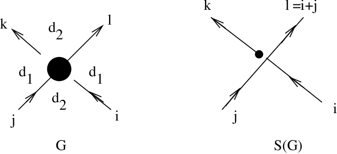
are associated to the crossings of 𝒢\displaystyle{\mathcal{G}} with signs ∗b=+1\displaystyle*_{b}=+1 and ∗b=−1\displaystyle*_{b}=-1, respectively, as on the left of Figure 3 and Figure 4, where i,j,k,l∈ℐN\displaystyle i,j,k,l\in{\mathcal{I}}_{N} label the edges of 𝒢\displaystyle{\mathcal{G}}.

Refer to caption
Figure 3. Matrix dilogarithm and S-graph: ∗b=1\displaystyle*_{b}=1.
Refer to caption
Figure 4. Matrix dilogarithm and S-graph: ∗b=−1\displaystyle*_{b}=-1.

We call a state of 𝒢\displaystyle{\mathcal{G}} any labeling of its edges by indices in ℐN\displaystyle{\mathcal{I}}_{N}. Every state s\displaystyle s selects an entry of ℛN​(Δ,b,d)\displaystyle{\mathcal{R}}_{N}(\Delta,b,d), denoted by ℛN​(s,Δ,b,d)\displaystyle{\mathcal{R}}_{N}(s,\Delta,b,d), at every crossing of 𝒢\displaystyle{\mathcal{G}}. The QH state sum ℋN​(𝒯)\displaystyle{\mathcal{H}}_{N}({\mathcal{T}}) is defined by tracing (ie. contracting indices) the resulting tensor network carried by 𝒢\displaystyle{\mathcal{G}}:

(2) ℋN​(𝒯)=N−(V−2)​∑s∏(Δ,b,d)ℛN​(s,Δ,b,d){\mathcal{H}}_{N}({\mathcal{T}})=N^{-(V-2)}\sum_{s}\prod_{(\Delta,b,d)}{\mathcal{R}}_{N}(s,\Delta,b,d)

where V\displaystyle V is the number of vertices of T\displaystyle T that are manifold points.

Remarks 2.2.

(1) We will use graphical as well as litteral representations of tensors. Time by time, we must fix carefully the encoding/decoding rules in order to pass from one representation to the other. A first example is shown in Figure 3 and Figure 4:

Convention. The indices associated to ingoing (outgoing) arrows in a graphical representation correspond to top (bottom) indices in the litteral representation.

(2) In [3, 4, 5] we used the normalization factor N−V\displaystyle N^{-V}. The present choice is more convenient to deal with the QH link invariants, as it yields ℋN​(KU)=1\displaystyle{\mathcal{H}}_{N}(K_{U})=1 for every N\displaystyle N (see Lemma 6.8).

We refer to Section 6 for the explicit formulas of the N\displaystyle N-matrix dilogarithms. We just recall here that the non vanishing entries ℛN​(s,Δ,b,d)\displaystyle{\mathcal{R}}_{N}(s,\Delta,b,d) depend on the N\displaystyle Nth root cross ratios w0′,w1′\displaystyle w^{\prime}_{0},w^{\prime}_{1} given in (1), and correspond to indices satisfying i+j=l\displaystyle i+j=l (N)\displaystyle(N).

Define 𝒮⁡(𝒢,N)\displaystyle{\mathcal{S}}({\mathcal{G}},N) as the set of efficient states, such that ℛN​(s,Δ,b,d)≠0\displaystyle{\mathcal{R}}_{N}(s,\Delta,b,d)\neq 0 for all Δ\displaystyle\Delta in T\displaystyle T. We have 𝒮⁡(𝒢,N)=H1​(S⁡(𝒢),∂S⁡(𝒢),ℐN)\displaystyle{\mathcal{S}}({\mathcal{G}},N)=H_{1}(S({\mathcal{G}}),\partial S({\mathcal{G}});\ {\mathcal{I}}_{N}), where the S-graph S⁡(𝒢)\displaystyle S({\mathcal{G}}) is the oriented (branched) graph with either 1-valent or 3-valent vertices, obtained from 𝒢\displaystyle{\mathcal{G}} by performing at each vertex the modification shown on the right of Figure 3 and Figure 4; the 1-valent vertices form the boundary ∂S⁡(𝒢)\displaystyle\partial S({\mathcal{G}}). Hence S⁡(𝒢)\displaystyle S({\mathcal{G}}) determines the actual range of summation in (2), and governs the state sum ℋN​(𝒯)\displaystyle{\mathcal{H}}_{N}({\mathcal{T}}).

2.3. From link diagrams to 3\displaystyle 3-dimensional triangulations

There is a very simple tunnel construction, introduced for instance in Example 4.3 of [3], that associates to a link diagram a branched triangulation of S3\displaystyle S^{3}. It is very convenient to describe this construction in terms of o-graphs.

Let 𝒟\displaystyle{\mathcal{D}} be a link diagram on ℝ2⊂ℝ2∪∞=S2\displaystyle{\mathbb{R}}^{2}\subset{\mathbb{R}}^{2}\cup\infty=S^{2}, representing a link L\displaystyle L. We assume that 𝒟\displaystyle{\mathcal{D}} verifies the following further condition (that can be always achieved for every link L\displaystyle L):

Every connected component of S2∖|𝒟|\displaystyle S^{2}\setminus|{\mathcal{D}}| is an open 2\displaystyle 2-disk, and 𝒟\displaystyle{\mathcal{D}} has at least one crossing.

By |𝒟|\displaystyle|{\mathcal{D}}| we mean the planar graph obtained by forgetting the over/under crossings. The components of S2∖|𝒟|\displaystyle S^{2}\setminus|{\mathcal{D}}| are called 𝒟\displaystyle{\mathcal{D}}-regions.

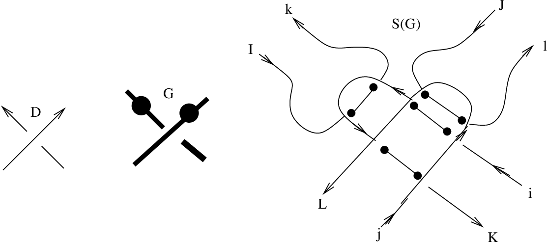
Figure 5 shows how to get from 𝒟\displaystyle{\mathcal{D}} two o-graphs G′\displaystyle G^{\prime} and G\displaystyle G by replacing every crossing and every edge with an o-graph portion. Both G\displaystyle G and G′\displaystyle G^{\prime} have no accidental virtual crossings.

Refer to caption
Figure 5. From link diagrams to o-graphs.

By forgetting the dots, the o-graph G′\displaystyle G^{\prime} appears as the superposition of two oppositely oriented copies of the link diagram 𝒟\displaystyle{\mathcal{D}}. It encodes a branched triangulation (T′,b′)\displaystyle(T^{\prime},b^{\prime}) of the pseudo-manifold Z⁡(L)\displaystyle Z(L), with 4​C\displaystyle 4C tetrahedra (C\displaystyle C being the number of crossings of 𝒟\displaystyle{\mathcal{D}}), E\displaystyle E non-manifold vertices (E\displaystyle E being the number of components of L\displaystyle L), and 2\displaystyle 2 further manifold vertices V±\displaystyle V_{\pm}. The o-graph G\displaystyle G encodes a branched triangulation (T,b)\displaystyle(T,b) of S3\displaystyle S^{3}, with 8​C\displaystyle 8C tetrahedra; the vertices V±\displaystyle V_{\pm} persist in T\displaystyle T, and there are 2​C\displaystyle 2C further vertices.

Let us describe these triangulations. Start with

S2×[−1,1]=S3∖(B3​(−)∪B3​(+))⊂S3S^{2}\times[-1,1]=S^{3}\setminus(B^{3}(-)\cup B^{3}(+))\subset S^{3}

where B3​(±)\displaystyle B^{3}(\pm) is an open 3\displaystyle 3-ball with boundary S2×{±1}\displaystyle S^{2}\times\{\pm 1\}. Identify ℝ2⊂ℝ2∪∞=S2\displaystyle{\mathbb{R}}^{2}\subset{\mathbb{R}}^{2}\cup\infty=S^{2} with S2×{0}\displaystyle S^{2}\times\{0\}, which is a non singular spine of S2×[−1,1]\displaystyle S^{2}\times[-1,1]. The over/under crossings of the diagram 𝒟\displaystyle{\mathcal{D}} are thus specified with respect to the coordinate t\displaystyle t on [−1,1]\displaystyle[-1,1].

The o-graph G′\displaystyle G^{\prime} encodes a standard branched spine (P′,b^′)\displaystyle(P^{\prime},\hat{b}^{\prime}) of S2×[−1,1]∖U⁡(L)\displaystyle S^{2}\times[-1,1]\setminus U(L), where U⁡(L)\displaystyle U(L) is an open tubular neighbourhood of L\displaystyle L. The vertices V±\displaystyle V_{\pm} correspond to the centers of B3​(±)\displaystyle B^{3}(\pm). In fact P′\displaystyle P^{\prime} is obtained by “digging a tunnel” in S2×[−1,1]\displaystyle S^{2}\times[-1,1] along L\displaystyle L, by following the diagram 𝒟\displaystyle{\mathcal{D}}. There is a natural bijection between the 𝒟\displaystyle{\mathcal{D}}-regions of the link diagram and the 2\displaystyle 2-regions of P′\displaystyle P^{\prime} contained in S2\displaystyle S^{2}, that we also call 𝒟\displaystyle{\mathcal{D}}-regions.

The o-graph G\displaystyle G encodes a standard branched spine (P,b^)\displaystyle(P,\hat{b}) obtained from (P′,b^′)\displaystyle(P^{\prime},\hat{b}^{\prime}) by inserting a wall in the tunnel digged about every edge of |𝒟|\displaystyle|{\mathcal{D}}|; topologically, each wall is a meridian 2\displaystyle 2-disk of U⁡(L)\displaystyle U(L). In order to extend the branching we have to fix the wall orientations. Both choices are admissible; at the bottom of Figure 5 we show the two possibilities for G\displaystyle G. Later we will fix a choice by using an auxiliary diagram orientation. The vertices V±\displaystyle V_{\pm} persist in the dual triangulation (T,b)\displaystyle(T,b) and the 𝒟\displaystyle{\mathcal{D}}-regions persist in (P,b^)\displaystyle(P,\hat{b}). There is also a partition by pairs of the further 2​C\displaystyle 2C vertices of T\displaystyle T produced by the walls. Every pair, say (v−,v+)\displaystyle(v^{-},v^{+}), is associated to a crossing of 𝒟\displaystyle{\mathcal{D}}. The two vertices of each pair are separated by the spine S2×{0}\displaystyle S^{2}\times\{0\} of S2×[−1,1]\displaystyle S^{2}\times[-1,1], and are the endpoints of an oriented edge [v−,v+]\displaystyle[v^{-},v^{+}] of (T,b)\displaystyle(T,b).

The triangulation (T,b)\displaystyle(T,b) has the following further properties:

(P1) It is quasi-regular, that is, every edge of T\displaystyle T has endpoints at distinct vertices.

(P2) The edges of T\displaystyle T dual to the walls realise L\displaystyle L as a subcomplex H′\displaystyle H^{\prime} of the 1\displaystyle 1-skeleton of T\displaystyle T, containing all the further 2​C\displaystyle 2C vertices of T\displaystyle T but missing V±\displaystyle V_{\pm}.

The definition of G′\displaystyle G^{\prime} works as well if 𝒟\displaystyle{\mathcal{D}} is the unknot diagram without crossing; in such a case we stipulate that G\displaystyle G is obtained from G′\displaystyle G^{\prime} by inserting two walls.

Remark 2.3.

If we insert several parallel oriented walls (more than one) around every edge of |𝒟|\displaystyle|{\mathcal{D}}|, we get branched triangulations of S3\displaystyle S^{3}, with more vertices, satisfying similar properties.

To simplify the figures sometimes we will indicate the o-graph G\displaystyle G by means of fat diagrams, with black disks corresponding to the walls of G\displaystyle G (the wall orientations will be specified time by time). See Figure 6.

2.4. Links carried by a link diagram

Let 𝒟\displaystyle{\mathcal{D}}, (P,b^)\displaystyle(P,\hat{b}) and (T,b)\displaystyle(T,b) be as in Section 2.3. We indicate now two ways of selecting a Hamiltonian subcomplex H0\displaystyle H^{0} of the 1\displaystyle 1-skeleton of T\displaystyle T, that is, containing all the vertices of T\displaystyle T (recall that in (P2) above, the subcomplex H′\displaystyle H^{\prime} realizing L\displaystyle L is not Hamiltonian since V±∉H′\displaystyle V_{\pm}\notin H^{\prime}):

(i) There is one 𝒟\displaystyle{\mathcal{D}}-region of P\displaystyle P, say Ω0\displaystyle\Omega_{0}, that contains ∞∈S2\displaystyle\infty\in S^{2}. Select a wall B0\displaystyle B_{0} adjacent to Ω0\displaystyle\Omega_{0}. Select two edges of T\displaystyle T dual to regions adjacent to B0\displaystyle B_{0} and located at opposite sides of it, such that one has V+\displaystyle V_{+} and the other V−\displaystyle V_{-} as an endpoint. Remove from H′\displaystyle H^{\prime} the interior of the edge dual to B0\displaystyle B_{0}, and take the union of the resulting triangulated arc with the two selected edges, and the edge dual to Ω0\displaystyle\Omega_{0}. We get a complex H0\displaystyle H^{0} that is Hamiltonian and provides (up to isotopy) another realization of L\displaystyle L. We denote it by L0\displaystyle L^{0}.

(ii) Select two 𝒟\displaystyle{\mathcal{D}}-regions of G\displaystyle G. The dual edges have V+\displaystyle V_{+} and V−\displaystyle V_{-} as endpoints, and their union realizes an unknot K\displaystyle K in S3\displaystyle S^{3}, possibly linked with L\displaystyle L. Take H0=H′∪K\displaystyle H^{0}=H^{\prime}\cup K. It realizes a link L0=L∪K\displaystyle L^{0}=L\cup K.

Definition 2.4.

For every link diagram 𝒟\displaystyle{\mathcal{D}}, any link L0\displaystyle L^{0} obtained either as in (i) or (ii) is said to be carried by 𝒟\displaystyle{\mathcal{D}}.

In Figure 6 we show some example of links carried by diagrams. As indicated after Remark 2.3, fat diagrams correspond to o-graphs. The two distinguished regions involved in the implementation of (ii) are labeled by “∗\displaystyle*”. So in case (a) L=KU\displaystyle L=K_{U}, the unknot, while L∪K\displaystyle L\cup K is the Hopf link. In case (b) again L=KU\displaystyle L=K_{U}, while L∪K\displaystyle L\cup K is the link 412\displaystyle 4^{2}_{1}, according to the Rolfsen table. In case (c) we have KU\displaystyle K_{U} versus the Whitehead link LW\displaystyle L_{W}, and in case (d) the Hopf link versus the link 613\displaystyle 6^{3}_{1} (the chain link). When a link is of the form L0=L∪K\displaystyle L^{0}=L\cup K where K\displaystyle K is an unknotted component, the procedure (ii) applied to a (suitable) diagram of L\displaystyle L often produces the most economic triangulations of S3\displaystyle S^{3} having L0\displaystyle L^{0} realized as a Hamiltonion subcomplex.

Refer to caption
Figure 6. Some links carried by diagrams.

From now on we always denote by L0\displaystyle L^{0} a link carried by a diagram 𝒟\displaystyle{\mathcal{D}}, hence obtained from (T,b,H0)\displaystyle(T,b,H^{0}) as above.

2.5. From link diagrams to distinguished QH triangulations

The next task is to convert (T,b,H0)\displaystyle(T,b,H^{0}) into a distinguished QH triangulation suited to the computation of the quantum hyperbolic invariants ℋN​(L0)\displaystyle{\mathcal{H}}_{N}(L^{0}).

Let (T,b,d)\displaystyle(T,b,d), d=(w,f,c)\displaystyle d=(w,f,c), be any QH triangulation supported by (T,b)\displaystyle(T,b). We define the total decoration of an edge e\displaystyle e of T\displaystyle T as

d⁡(e)=(W⁡(e),L⁡(e),C⁡(e))d(e)=(W(e),L(e),C(e))

where W⁡(e)\displaystyle W(e) is the product over all tetrahedra glued along e\displaystyle e of the (wj′)∗b\displaystyle(w_{j}^{\prime})^{*_{b}}s at e\displaystyle e (the N\displaystyle Nth root cross-ratio moduli or their inverses according to ∗b=±1\displaystyle*_{b}=\pm 1), and L⁡(e)\displaystyle L(e) and C⁡(e)\displaystyle C(e) are the similar sums of signed log-branches ∗blj\displaystyle*_{b}l_{j} and cj\displaystyle c_{j}s, respectively. The total decoration d⁡(R)\displaystyle d(R) of a spine 2\displaystyle 2-region R\displaystyle R is defined in a dual way. We are going to impose to (T,b,d)\displaystyle(T,b,d) global constraints in terms of H0\displaystyle H^{0} and the d⁡(e)\displaystyle d(e)s (see [3, 4, 5] for details).

Global conditions on (w,f)\displaystyle(w,f). These do not depend on H0\displaystyle H^{0}. First we want the cross-ratios to encode the trivial representation ρtriv\displaystyle\rho_{\rm triv}. It is enough to require that

(3) W⁡(e)=1,forevery​edge​e.W(e)=1,\ \ {\rm for\ \ every\ edge}\ e.

Moreover, we also require that

(4) L⁡(e)=0,forevery​edge​e.L(e)=0,\ \ {\rm for\ \ every\ edge}\ e.

Global charges. The global conditions on charges encode the subcomplex H0\displaystyle H^{0} of T\displaystyle T. They are

(5) {C⁡(e)=0for​every​e∈H0C⁡(e)=2for​every​e∈T∖H0.\left\{\begin{array}[]{ll}C(e)=0&{\rm for\ every}\ e\in H^{0}\\ C(e)=2&{\rm for\ every}\ e\in T\setminus H^{0}.\end{array}\right.

We call distinguished any QH triangulation 𝒯=(T,H0,b,d)\displaystyle{\mathcal{T}}=(T,H^{0},b,d) satisfying the global constraints (3), (4) and (5). We denote by 𝒢=𝒢⁡(𝒟,H0)\displaystyle{\mathcal{G}}={\mathcal{G}}({\mathcal{D}},H^{0}) the corresponding QH o-graph. It is a particular case of the general results of [3, 4] that, up to the determined phase ambiguity, the value of the state sum ℋN​(𝒯)\displaystyle{\mathcal{H}}_{N}({\mathcal{T}}) does not depend on the choice of the distinguished triangulation 𝒯\displaystyle{\mathcal{T}} so that ℋN​(𝒯)\displaystyle{\mathcal{H}}_{N}({\mathcal{T}}) well defines a link invariant ℋN​(L0)\displaystyle{\mathcal{H}}_{N}(L^{0}).

Now we use some specific features of (T,H0,b)\displaystyle(T,H^{0},b) in order to specialize the choice of 𝒯\displaystyle{\mathcal{T}}.

Universal constant system (w,f)\displaystyle(w,f). A nice property of the triangulations (T,b,H0)\displaystyle(T,b,H^{0}) is the existence of a constant system (w,f)\displaystyle(w,f) of cross ratios and flattenings that works for any diagram 𝒟\displaystyle{\mathcal{D}} and any choice of wall orientations. A solution is

(w0,f0,f1)=(2,0,−1),(l0,l1,l2)=(log⁡(2),0,−log⁡(2)).(w_{0},f_{0},f_{1})=(2,0,-1),\quad(l_{0},l_{1},l_{2})=(\log(2),0,-\log(2)).

The conditions (3) and (4) hold because along the boundary of every spine 2\displaystyle 2-region which is also a 𝒟\displaystyle{\mathcal{D}}-region there is an even number of cross-ratios w1=−1\displaystyle w_{1}=-1, and at every further spine 2\displaystyle 2-region there is a pattern of pairs (wj,lj)\displaystyle(w_{j},l_{j}) with opposite b\displaystyle b-signs ∗b\displaystyle*_{b}. Note that the same argument works if instead of (T,b)\displaystyle(T,b) we take a triangulation obtained by inserting an odd number of walls at every edge of |𝒟|\displaystyle|{\mathcal{D}}| (see Remark 2.3).

Convention. From now on we will use by default the above universal constant system (w,f)\displaystyle(w,f), so that only the charges are varying parameters.

However, we will find useful in Section 4 to use another, more general, way to make (T,b,H0)\displaystyle(T,b,H^{0}) a distinguished QH triangulation.

Idealization. Systems of cross-ratios verifying (3) can be obtain as follows. We identify (ℂ,+)\displaystyle({\mathbb{C}},+) with the subgroup of S​L​(2,ℂ)\displaystyle SL(2,{\mathbb{C}}) acting via Moëbius transformations as translations on ℂ⊂ℂ∪∞=ℙ1​(ℂ)\displaystyle{\mathbb{C}}\subset{\mathbb{C}}\cup\infty={\mathbb{P}}^{1}({\mathbb{C}}). The coboundary z\displaystyle z of any ℂ\displaystyle{\mathbb{C}}-valued 0\displaystyle 0-cochain on (T,b)\displaystyle(T,b) can thus be considered as a P​S​L​(2,ℂ)\displaystyle PSL(2,{\mathbb{C}})-valued 1\displaystyle 1-cocycle on (T,b)\displaystyle(T,b) that represents ρtriv\displaystyle\rho_{\rm triv}. If z\displaystyle z is nowhere vanishing (which is the case if the 0\displaystyle 0-cochain is injective, since T\displaystyle T is quasi-regular), we say that z\displaystyle z is idealizable (with base point 0\displaystyle 0). In such a case, if x0,x1,x2\displaystyle x_{0},x_{1},x_{2} and x3\displaystyle x_{3} are the vertices of a branched tetrahedron (Δ,b)\displaystyle(\Delta,b) of (T,b)\displaystyle(T,b), ordered by using the branching b\displaystyle b, we can define four distinct points of ℂ\displaystyle{\mathbb{C}} by

u0=0,u1=z⁡([x0,x1])​(0),u2=z⁡([x0,x2])​(0),u3=z⁡([x0,x3])​(0).u_{0}=0,\ u_{1}=z([x_{0},x_{1}])(0),\ u_{2}=z([x_{0},x_{2}])(0),\ u_{3}=z([x_{0},x_{3}])(0).

The associated cross-ratio is

w0=[u0:u1:u2:u3]=u3(u2−u1)/u2(u3−u1)∈ℂ∖{0,1}.w_{0}=[u_{0}:u_{1}:u_{2}:u_{3}]=u_{3}(u_{2}-u_{1})/u_{2}(u_{3}-u_{1})\in\mathbb{C}\setminus\{0,1\}.

Cross-ratios obtained in this way have so-called canonical log-branches, which satisfy condition (4):

(6) l0:=log⁡(u2−u1)+log⁡(u3)−log⁡(u2)−log⁡(u3−u1)l1:=log⁡(u2)+log⁡(u3−u1)−log⁡(u1)−log⁡(u3−u2)l2:=log⁡(u3−u2)+log⁡(u1)−log⁡(u3)−log⁡(u2−u1)\begin{array}[]{l}l_{0}:=\log(u_{2}-u_{1})+\log(u_{3})-\log(u_{2})-\log(u_{3}-u_{1})\\ l_{1}:=\log(u_{2})+\log(u_{3}-u_{1})-\log(u_{1})-\log(u_{3}-u_{2})\\ l_{2}:=\log(u_{3}-u_{2})+\log(u_{1})-\log(u_{3})-\log(u_{2}-u_{1})\end{array}

The corresponding canonical flattenings are fj:=(lj−log⁡(wj))/−1​π\displaystyle f_{j}:=(l_{j}-\log(w_{j}))/\sqrt{-1}\pi. Note that canonical flattenings are even, in the sense that both f0\displaystyle f_{0} and f1\displaystyle f_{1} belong to 2​ℤ\displaystyle 2{\mathbb{Z}}.

It is easy to see that any constant cross ratio-system on (T,b,H0)\displaystyle(T,b,H^{0}) can be obtained by idealization. For simplicity we will show it for knot diagrams, the general case being not much harder. Assume at first that the knot diagram 𝒟\displaystyle{\mathcal{D}} is alternating. We orient every wall in such a way that the dual oriented edge is of the form [v−,v+]\displaystyle[v^{-},v^{+}], where the two endpoints are possibly associated to different crossings of 𝒟\displaystyle{\mathcal{D}}. Note that this is possible because 𝒟\displaystyle{\mathcal{D}} is alternating. Next we fix a 0-cochain γ\displaystyle\gamma of the form:

γ⁡(V±)=±1,γ⁡(v±)=±a.\gamma(V_{\pm})=\pm 1,\quad\gamma(v^{\pm})=\pm a.

For a fixed generic a\displaystyle a the idealization procedure gives, at every tetrahedron (Δ,b)\displaystyle(\Delta,b) of (T,b)\displaystyle(T,b), the four points

(u0,u1,u2,u3)=(0,a−1,a+1,2​a)(u_{0},u_{1},u_{2},u_{3})=(0,a-1,a+1,2a)

with constant first cross-ratio

w0=4​a/(a+1)2.w_{0}=4a/(a+1)^{2}\ .

The corresponding canonical flattening is also constant. For example, w0=2\displaystyle w_{0}=2 iff a=±−1\displaystyle a=\pm\sqrt{-1}; if a=−1\displaystyle a=\sqrt{-1}, we get the constant canonical flattening (w0,f0,f1)=(2,0,−2)\displaystyle(w_{0},f_{0},f_{1})=(2,0,-2).

If 𝒟\displaystyle{\mathcal{D}} is not alternating, we can modify the above procedure as follows in order to obtain anyway any constant cross-ratio w0=4​a/(a+1)2\displaystyle w_{0}=4a/(a+1)^{2}.

Lemma 2.5.

Given any knot diagram 𝒟\displaystyle{\mathcal{D}}, there is a way to select a crossing segment at every double point of |𝒟|\displaystyle|{\mathcal{D}}| so that there is exactly one segment endpoint on each edge of |𝒟|\displaystyle|{\mathcal{D}}|.

Proof. Orient |𝒟|\displaystyle|{\mathcal{D}}|. Select one crossing segment at a double point, and move along |𝒟|\displaystyle|{\mathcal{D}}| according to the orientation. Pass across the next visited double point without selecting any segment, continue and select on the next visited double point the crossing segment according to our move along the graph. Continue by alternating in this way: “select”, “pass across”, “select”, “pass across”, etc. If we complete the circuit without obstructions we are done. Assume on the contrary that we reach a first obstruction. This means that, for the first time, either we visit again a double point with an already selected crossing segment, and the rule would impose that we should select now also the other crossing segment, or we visit again a double point with no selected crossing segment, and the rule would impose that we should again select no segment. In both situations we have created a loop in |𝒟|\displaystyle|{\mathcal{D}}| with an odd number of legs of crossings pointing into the encircled region. So there is one leg that is trapped. This is absurd. □\displaystyle\Box

Remark 2.6.

Lemma 2.5 is obviously true for any alternating knot diagram, and given a arbitrary knot diagram 𝒟\displaystyle{\mathcal{D}}, if we define 𝒟′\displaystyle{\mathcal{D}}^{\prime} by stipulating that every selected segment on |𝒟|\displaystyle|{\mathcal{D}}| is over-crossing, then 𝒟′\displaystyle{\mathcal{D}}^{\prime} is alternating. That is, Lemma 2.5 is equivalent to the fact that for every knot diagram 𝒟\displaystyle{\mathcal{D}} there is an alternating knot diagram 𝒟′\displaystyle{\mathcal{D}}^{\prime} such that |𝒟|=|𝒟′|\displaystyle|{\mathcal{D}}|=|{\mathcal{D}}^{\prime}|.

Now let 𝒟\displaystyle{\mathcal{D}} and 𝒟′\displaystyle{\mathcal{D}}^{\prime} be as in the last remark. Let γ′\displaystyle\gamma^{\prime} be the 0-cochain defined as above on the alternating diagram 𝒟′\displaystyle{\mathcal{D}}^{\prime}; then, by moving along |𝒟|\displaystyle|{\mathcal{D}}| as in the proof of Lemma 2.5, we define a 0-cochain γ\displaystyle\gamma on 𝒟\displaystyle{\mathcal{D}} such that γ=γ′\displaystyle\gamma=\gamma^{\prime} at every crossing where 𝒟\displaystyle{\mathcal{D}} and 𝒟′\displaystyle{\mathcal{D}}^{\prime} coincide, and

γ⁡(V±)=±1,γ⁡(v±)=−γ′​(v±)\gamma(V_{\pm})=\pm 1,\quad\gamma(v^{\pm})=-\gamma^{\prime}(v^{\pm})

elsewhere. It turns out that the idealization of γ\displaystyle\gamma has the constant w0=4​a/(a+1)2\displaystyle w_{0}=4a/(a+1)^{2}, as desired. However, note that the canonical flattening is not constant.

3. Enhanced QH Yang-Baxter operators

We deal with a triangulation (T,b)\displaystyle(T,b) associated to a diagram 𝒟\displaystyle{\mathcal{D}} of a link L\displaystyle L, according to the construction of Section 2.3. It is endowed with the universal constant system (w0,f0,f1)=(2,0,−1)\displaystyle(w_{0},f_{0},f_{1})=(2,0,-1), so that it remains to manage with the charge.

Notations for charge variables. For the aim of future computations, it is convenient to fix a name for the charge variables on 𝒢\displaystyle{\mathcal{G}}. In Figure 7 we show the charge variables

(R,S,U,V,A,B,C,E,Y,Z,T,X)(R,S,U,V,A,B,C,E,Y,Z,T,X)

at the four crossings of 𝒢\displaystyle{\mathcal{G}} corresponding to a crossing of 𝒟\displaystyle{\mathcal{D}}, and the charge variables

(P,F,H,M,G,K)(P,F,H,M,G,K)

at the two crossings of 𝒢\displaystyle{\mathcal{G}} corresponding to a wall. On the wall we have also indicated state variables i,j,k,l\displaystyle i,j,k,l for future use.

Refer to caption
Figure 7. Crossing and wall charge variables.

Because of the symmetries there is no way for the moment to fix the position of the variables A\displaystyle A rather than C\displaystyle C, and so on.

We refine the previous constructions by assuming that every link diagram 𝒟\displaystyle{\mathcal{D}} is endowed with an auxiliary orientation. We use the orientation in order to:

(O1) Fix the wall orientations according to the convention of Figure 8.

Refer to caption
Figure 8. Wall orientation.

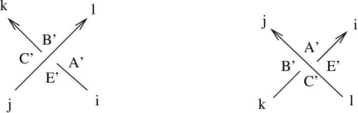
(O2) Fix the notations of the charge variables at each crossing according to the convention of Figure 9. Here we show only the labelings of the four germs of 𝒟\displaystyle{\mathcal{D}}-regions at a crossing. The other labelings follow in agreement with Figure 7.

Refer to caption
Figure 9. Charge labeling via oriented diagrams.

(O3) Fix a partition by pairs of the walls of the triangulation (T,b)\displaystyle(T,b): each pair is made of two walls located at the outgoing edges of a crossing of 𝒟\displaystyle{\mathcal{D}}.

3.1. Specialization to closed braids and Yang-Baxter charges

Suppose now that 𝒟\displaystyle{\mathcal{D}} is the closure of a braid ℬ\displaystyle{\mathcal{B}}. We stipulate that:

Convention. braids are vertical and directed from bottom to top, with the closing arcs on the right.

Hence 𝒟\displaystyle{\mathcal{D}} is oriented. Every closing arc has one maximum and one minimum with respect to the vertical direction.

Modify the triangulation (T,b)\displaystyle(T,b) associated to 𝒟\displaystyle{\mathcal{D}} by inserting a further wall at each such maximum/minimum point, oriented by the rule of Figure 8; these walls are indicated by black squares on fat diagrams (see Figure 10). As for (T,b)\displaystyle(T,b), the edges of the resulting triangulation (T′,b′)\displaystyle(T^{\prime},b^{\prime}), which are dual to the walls make a non Hamiltonian subcomplex H′\displaystyle H^{\prime} realizing L\displaystyle L. The universal constant system (w,f)\displaystyle(w,f) works as well on (T′,b′)\displaystyle(T^{\prime},b^{\prime}).

We are going to define a family of charges made up from local constant pieces associated to the crossings and the walls on the (oriented) fat diagrams of the o-graph 𝒢′\displaystyle{\mathcal{G}}^{\prime} corresponding to (T′,b′)\displaystyle(T^{\prime},b^{\prime}). By using the above orientation conventions (O1)–(O3) and those of Figure 7, we denote the charge variables as follows:

(7) {(R​1,S​1,…,A​1,B​1,C​1,E​1)​at​every​𝑝𝑜𝑠𝑖𝑡𝑖𝑣𝑒​crossing;(R​2,S​2,…,A​2,B​2,C​2,E​2)​at​every​𝑛𝑒𝑔𝑎𝑡𝑖𝑣𝑒​crossing;(P,F,H,M,−F,K)​at​every​wall​associated​to​a​crossing;(P​1,F​1=−1,H​1,M​1,G​1=1,K​1)​at​every​wall​associated​to​a​maximum;(P​2,F​2=−1,H​2,M​2,G​2=1,K​2)​at​every​wall​associated​to​a​minimum.\left\{\begin{array}[]{l}(R1,S1,\dots,A1,B1,C1,E1)\ {\rm at\ every\ {\it positive}\ crossing};\\ (R2,S2,\dots,A2,B2,C2,E2)\ {\rm at\ every\ {\it negative}\ crossing};\\ (P,F,H,M,-F,K)\ {\rm at\ every\ wall\ associated\ to\ a\ crossing};\\ (P1,F1=-1,H1,M1,G1=1,K1)\ {\rm at\ every\ wall\ associated\ to\ a\ maximum};\\ (P2,F2=-1,H2,M2,G2=1,K2)\ {\rm at\ every\ wall\ associated\ to\ a\ minimum}.\end{array}\right.

Next we are going to impose invariance of (7) under the stabilization moves, a braid Reidemeister move III and a composition of braid Reidemeister moves II. See the figures 10, 11 and 12.

Refer to caption
Figure 10. Stabilization.
Refer to caption
Figure 11. Braid Reidemeister move II.
Refer to caption
Figure 12. Braid Reidemeister move III.

In every case we have two portions of fat diagrams of QH o-graphs, supporting portions of QH branched spines. The two portions of spines carry sets of 2\displaystyle 2-regions “with boundary” corresponding to edges of T′\displaystyle T^{\prime} with incomplete star, which are in natural 1-1 correspondence one to each other, and some internal 2\displaystyle 2-regions, corresponding to edges having complete star. The invariance of the charge variables (7) should be a consequence of QH transits relating the portions of QH branched spines, in the sense of [3, 4, 5]. Equivalently:

  • •

    Corresponding regions with boundary have the same total charge;

  • •

    Each internal region has total charge equal to 2\displaystyle 2.

First we study these conditions on the 𝒟\displaystyle{\mathcal{D}}-regions, that is, for the charge variables that appear in the (planar) figures. Then we will see how these lift to conditions on the whole charges.

The stabilization moves (i.e. the Reidemeister moves I) lead to the set of independent conditions

(8) B​2+2​F=0,A​2+B​2+C​2+E​2=2,C​2−2+A​2=0,C​1+2​F=0,A​1+B​1+C​1+E​1=2,E​1−2+B​1=0.\begin{array}[]{llll}B2+2F=0,&A2+B2+C2+E2=2,&C2-2+A2=0,\\ C1+2F=0,&A1+B1+C1+E1=2,&E1-2+B1=0.\end{array}

Note that the maxima/minima walls (having F=−1\displaystyle F=-1, G=1\displaystyle G=1) contribute to get a total charge equal to 2\displaystyle 2 on the internal 𝒟\displaystyle{\mathcal{D}}-region created by the curl.

Consider a composition of two opposite Reidemeister moves II (recall our convention on link diagrams in Section 2.3). It gives a further independent condition,

(9) B​1+C​2=2.B1+C2=2.

The Reidemeister move III yields, in turn, F=0\displaystyle F=0. Then, the system (8) & (9) has the one-parameter family of solutions

(10) A​1=C​1=0,B​1+E​1=2,B​2=E​2=0,B​1=A​2,E​1=C​2,F=0.A1=C1=0,\quad B1+E1=2,\quad B2=E2=0,\quad B1=A2,\quad E1=C2,\quad F=0.

It works also for all other instances of Reidemeister moves III.

Next we have to prove the existence of charges on (T′,H′)\displaystyle(T^{\prime},H^{\prime}) satisfying (10). Recall the condition (C3) in Section 2.1, that will be always assumed. By using the above solution, at crossings we have:

X​1=−1−V​1+B​1,Y​1=1−R​1,Z​1=1−S​1−B​1,T​1=1−U​1,X​2=1−V​2,Y​2=1−R​2−B​1,Z​2=1−S​2,T​2=−1−U​2+B​1.\begin{array}[]{cccc}X1=-1-V1+B1,&Y1=1-R1,&Z1=1-S1-B1,&T1=1-U1,\\ X2=1-V2,&Y2=1-R2-B1,&Z2=1-S2,&T2=-1-U2+B1.\end{array}

At walls we have

(11) H=1−P,H​1=2−P​1,H​2=2−P​2K=1−M,K​1=−M​1,K​2=−M​2.\begin{array}[]{lll}H=1-P,&H1=2-P1,&H2=2-P2\\ K=1-M,&K1=-M1,&K2=-M2.\end{array}

The composition of Reidemeister moves II and the positive curl introduce respectively the independent relations

T​1+Z​1=T​1+X​1=2−(P+M),Y​1+Z​1=X​1+Y​1=P+MT​2+X​2=X​2+Y​2=2−(P+M),T​2+Z​2=Y​2+Z​2=P+MU1+V1+S1+R1=0,U2+V2+S2+R2=0,\begin{array}[]{c}T1+Z1=T1+X1=2-(P+M),\quad Y1+Z1=X1+Y1=P+M\\ T2+X2=X2+Y2=2-(P+M),\quad T2+Z2=Y2+Z2=P+M\\ U1+V1+S1+R1=0,\quad U2+V2+S2+R2=0,\end{array}

and

P+M+H​2+K​2=P​1+M​1+H+K=2P​2+M​2+H​1+K​1=P​2+M​2+X​2+T​2=2.\begin{array}[]{c}P+M+H2+K2=P1+M1+H+K=2\\ P2+M2+H1+K1=P2+M2+X2+T2=2.\end{array}

Together with (11) the latter yields

P+M=H+K=P​1+M​1=H​1+K​1=P​2+M​2=H​2+K​2.P+M=H+K=P1+M1=H1+K1=P2+M2=H2+K2.

Finally we realize that neither the negative curl nor the Reidemeister move III add independent relations. Summing up the above computations we get:

Proposition 3.1.

The variables (7) lift to a global charge on the triangulation (T′,H′)\displaystyle(T^{\prime},H^{\prime}) which is invariant with respect to the Reidemeister moves I and III and the composition of Reidemeister moves of Figures 11, if and only the following relations, depending on the free parameters (U​1,U​2,B​1,P,P​1,P​2)\displaystyle(U1,U2,B1,P,P1,P2), hold true:

R​1=U​1,S​1=1−B​1−U​1,V​1=B​1−U​1−1A​1=0,C​1=0,B​1+E​1=2R​2=2+U​2−2​B​1,S​2=−1−U​2+B​1,V​2=S​2B​2=0,E​2=0,A​2=B​1,C​2=E​1F=0,M=1−P,G=0F​1=−1,M​1=1−P​1,G​1=1F2=−1,M2=1−P2,G2=1.\begin{array}[]{c}R1=U1,\quad S1=1-B1-U1,\quad V1=B1-U1-1\\ A1=0,\quad C1=0,\quad B1+E1=2\\ R2=2+U2-2B1,\quad S2=-1-U2+B1,\quad V2=S2\\ B2=0,\quad E2=0,\quad A2=B1,\quad C2=E1\\ F=0,\quad M=1-P,\quad G=0\\ F1=-1,\quad M1=1-P1,\quad G1=1\\ F2=-1,\quad M2=1-P2,\quad G2=1.\end{array}

We call Yang-Baxter charge any of these solutions.

3.2. From Yang-Baxter charges to QH link invariants

Denote by 𝒯⁡(ℬ,c)\displaystyle{\mathcal{T}}({\mathcal{B}},c) the QH triangulation of S3\displaystyle S^{3} given by (T′,H′,b′)\displaystyle(T^{\prime},H^{\prime},b^{\prime}), a fixed Yang-Baxter charge c\displaystyle c, and the universal constant system (w,f)\displaystyle(w,f) of cross-ratio moduli and flattenings.

The QH triangulation 𝒯⁡(ℬ,c)\displaystyle{\mathcal{T}}({\mathcal{B}},c) is not distinguished for (S3,L)\displaystyle(S^{3},L). In fact, every edge of the subcomplex H′\displaystyle H^{\prime} realizing L\displaystyle L has total charge equal to 0\displaystyle 0, while the other edges have total charge equal to 2\displaystyle 2, with the exception of the edge dual to the region Ω0\displaystyle\Omega_{0}, which has total charge equal to −2\displaystyle-2. Hence ℋN​(𝒯​(ℬ,c))\displaystyle{\mathcal{H}}_{N}({\mathcal{T}}({\mathcal{B}},c)) is not a state sum of the quantum hyperbolic invariant ℋN​(L)\displaystyle{\mathcal{H}}_{N}(L). However, by recalling the constructions (i) and (ii) in Section 2.4, there are two natural ways to modify 𝒯⁡(ℬ,c)\displaystyle{\mathcal{T}}({\mathcal{B}},c) in order to get QH link invariants. The first is contained in the following lemma.

Lemma 3.2.

By inserting two new walls after the minimum/maximun ones at the closing arc adjacent to the region Ω0\displaystyle\Omega_{0}, the QH triangulation 𝒯⁡(ℬ,c)\displaystyle{\mathcal{T}}({\mathcal{B}},c) can be extended to a distinguished one 𝒯′​(ℬ,c′)\displaystyle{\mathcal{T}}^{\prime}({\mathcal{B}},c^{\prime}), such that ℋN(L)=NℋN(𝒯′(ℬ,c′))\displaystyle{\mathcal{H}}_{N}(L)=_{N}{\mathcal{H}}_{N}({\mathcal{T}}^{\prime}({\mathcal{B}},c^{\prime})).

Proof. The universal constant system (w,f)\displaystyle(w,f) extends to the two new walls, so that it remains to fix the charges on them. We do it as follows. The first wall (according to the arc orientation) carries the same charges as black disk walls at crossings; the second wall carries charges of the form

(P​0,F​0)=(P​0,2),(M​0,G​0)=(M​0,0)(P0,F0)=(P0,2),\quad(M0,G0)=(M0,0)

satisfying

P​0+M​0+1=0,1+H​0+K​0=2.P0+M0+1=0,\quad 1+H0+K0=2.

By the basic charge condition (3) of Section 2.1 this reduces to M​0=−P​0−1\displaystyle M0=-P0-1. Any extension c′\displaystyle c^{\prime} of c\displaystyle c is then determined by such a choice of P0\displaystyle P_{0} and M0\displaystyle M_{0}. □\displaystyle\Box

In Figure 13 we represent both 𝒯⁡(ℬ,c)\displaystyle{\mathcal{T}}({\mathcal{B}},c) (by forgetting the added dots near the region Ω0\displaystyle\Omega_{0}) and 𝒯′​(ℬ,c′)\displaystyle{\mathcal{T}}^{\prime}({\mathcal{B}},c^{\prime}) for a closed braid presentation of the Whitehead link. Values of a specific Yang-Baxter charge c\displaystyle c on the 𝒟\displaystyle{\mathcal{D}}-regions are indicated (B​1=2\displaystyle B1=2 and the F=0\displaystyle F=0 values on the black disk walls at crossings are omitted).

Refer to caption
Figure 13. The distinguished QH triangulation 𝒯′​(ℬ,c′)\displaystyle{\mathcal{T}}^{\prime}({\mathcal{B}},c^{\prime}) for the Whitehead link.

The second way is contained in the following lemma.

Lemma 3.3.

By removing from 𝒯⁡(ℬ,c)\displaystyle{\mathcal{T}}({\mathcal{B}},c) the maximum/minimum walls on the closing arc adjacent to the region Ω0\displaystyle\Omega_{0}, we get a distinguished QH triangulation 𝒯′′​(ℬ,c′′)\displaystyle{\mathcal{T}}^{\prime\prime}({\mathcal{B}},c^{\prime\prime}) (c′′\displaystyle c^{\prime\prime} being the restriction of c\displaystyle c) that carries the link L0=L∪Km\displaystyle L^{0}=L\cup K_{m}, where Km\displaystyle K_{m} is the meridian of the component of L\displaystyle L that contains that arc. Hence ℋN(𝒯′′(ℬ,c′′))=NℋN(L0)=NNℋN(L)\displaystyle{\mathcal{H}}_{N}({\mathcal{T}}^{\prime\prime}({\mathcal{B}},c^{\prime\prime}))=_{N}{\mathcal{H}}_{N}(L^{0})=_{N}N{\mathcal{H}}_{N}(L). In particular this does not depend on the choice of the component of L\displaystyle L supporting the meridian K\displaystyle K.

All the statements are clear with the exception of the last one, which is a consequence of Lemma 3.8 (2) below.

Remark 3.4.

The above results hold as well when 𝒟\displaystyle{\mathcal{D}} is more generally the closure of any oriented (1,1)\displaystyle(1,1)-tangle diagram in normal position with respect to the vertical direction (that is, all crossings are directed from bottom to top like for braids). Every (1,1)\displaystyle(1,1) tangle can be normalized by possibly rotating some crossing and introducing maxima/minima. Braid presentations correspond to special (1,1)\displaystyle(1,1)-tangles obtained by re-opening the closing arc adjacent to the region Ω0\displaystyle\Omega_{0}.

Finally we can consider also the state sum ℋN​(𝒯​(ℬ,c))\displaystyle{\mathcal{H}}_{N}({\mathcal{T}}({\mathcal{B}},c)) itself. The general invariance properties of QH state sums imply that its value does not depend on the choice of the closed braid 𝒟\displaystyle{\mathcal{D}} and the Yang-Baxter charge c\displaystyle c, up to the usual phase ambiguity. Hence we formally dispose of further link invariants, say

[L]N=ℋN​(𝒯⁡(ℬ,c)).[L]_{N}={\mathcal{H}}_{N}({\mathcal{T}}({\mathcal{B}},c)).

3.3. From Yang-Baxter charges to enhanced Yang-Baxter operators

In order to finalize the discussion, we fix now the following specific Yang-Baxter charge c0\displaystyle c_{0}:

R​1=U​1=0,S​1=−1,V​1=1,A​1=0,C​1=0,E​1=0,B​1=2R1=U1=0,\ S1=-1,\ V1=1,\ A1=0,\ C1=0,\ E1=0,B1=2
R​2=−2,U​2=0,S​2=1,V​2=1,B​2=0,E​2=0,A​2=2,C​2=0R2=-2,\ U2=0,\ \ S2=1,\ V2=1,\ B2=0,\ E2=0,\ A2=2,\ C2=0
F=0,P=0,M=1,G=0F=0,\ P=0,\ M=1,\ G=0
Fj=−1,Pj=0Mj=1,Gj=1,j=1,2.Fj=-1,\ Pj=0\ Mj=1,\ Gj=1,\ \ j=1,2\ .

Similarly, in Lemma 3.2 we fix P​0=0\displaystyle P0=0. Note, however, that the following discussion works as well for any Yang-Baxter charge c\displaystyle c.

On the QH o-graph 𝒢\displaystyle{\mathcal{G}} corresponding to 𝒯⁡(ℬ,c0)\displaystyle{\mathcal{T}}({\mathcal{B}},c_{0})), we point out a few distinguished local configurations:

Walls: There are two types of walls, either near a crossing or at a maximum/minimum. We call them C-wall and M-wall respectively.

Crossings: At every positive (negative) crossing we distinguish two local configurations, called braiding and complete crossing respectively.

For every odd N\displaystyle N, every such a local portion of 𝒢\displaystyle{\mathcal{G}} supports a QH tensor in the following sense:

Definition 3.5.

The local QH tensor of a portion of 𝒢\displaystyle{\mathcal{G}} is the result of tracing, like in formula (2), the pattern of matrix dilogarithms associated to 𝒢\displaystyle{\mathcal{G}}, and normalizing by a factor N−1\displaystyle N^{-1} for each wall (hence “complete crossings” below are normalized by a factor N−2\displaystyle N^{-2}).

The local QH tensors can be read directly from the diagram 𝒟\displaystyle{\mathcal{D}}, and the normalization distributes the factor N−(V−2)\displaystyle N^{-(V-2)} in (2).

The “complete crossing” local portions (in terms of S-graphs), and the corresponding QH tensors (in graphical representation) are shown in Figure 14 and Figure 15; all state variables belong to ℐN\displaystyle{\mathcal{I}}_{N}.

Refer to caption
Figure 14. Positive complete crossing.
Refer to caption
Figure 15. Negative complete crossing.

The position of the state indices is somehow reminescent of the one for matrix dilogarithms in Figure 3 and Figure 4. The corresponding litteral notation for the same tensors will be respectively

(12) ℋN​(C,+)k,l,K,Li,j,I,J,ℋN​(C,−)i,j,I,Jk,l,K,L.{\mathcal{H}}_{N}(C,+)^{i,j,I,J}_{k,l,K,L}\ \ ,\ \ {\mathcal{H}}_{N}(C,-)_{i,j,I,J}^{k,l,K,L}\ .

To get the “braiding” local portions, we just eliminate the walls from Figure 14 and Figure 15 (thus getting pictures like on the left of Figure 7), and we keep the same state index distribution. The corresponding litteral notations will be respectively

(13) ℋN​(B,+)k,l,K,Li,j,I,J,ℋN​(B,−)i,j,I,Jk,l,K,L.{\mathcal{H}}_{N}(B,+)^{i,j,I,J}_{k,l,K,L}\ \ ,\ \ {\mathcal{H}}_{N}(B,-)_{i,j,I,J}^{k,l,K,L}\ .

Concerning the walls, we name the state variables as on the right of Figure 7. The corresponding litteral notation will be

(14) ℋN​(𝒲X)i,lj,k{\mathcal{H}}_{N}({\mathcal{W}}_{X})^{j,k}_{i,l}

where X=C,M\displaystyle X=C,M according to wall types. As the Yang-Baxter charge c0\displaystyle c_{0} is fixed, these local QH tensors are constant at every positive (resp. negative) crossing, and constant and equal at the maxima/minima.

Convention. We denote by “=N\displaystyle=_{N}” the equality of QH tensors modulo sign and multiplication by N\displaystyle Nth roots of unity that do not depend on states.

Let us anticipate some features of the QH enhanced Yang-Baxter operators (RN,MN,1,1)\displaystyle({\rm R}_{N},M_{N},1,1) that we are going to construct. They will include:

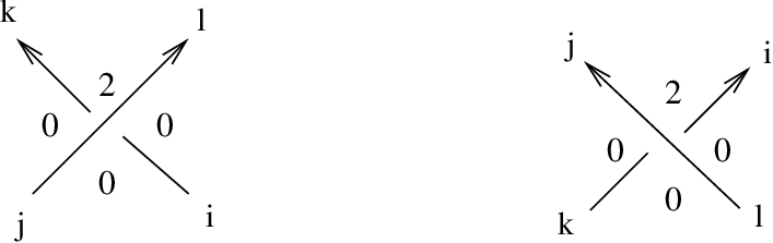
(1) The QH R-matrix RN=RN​(+)\displaystyle{\rm R}_{N}={\rm R}_{N}(+) with entries RN​(+)l,ki,j\displaystyle{\rm R}_{N}(+)_{l,k}^{i,j}, i,j,k,l∈ℐN\displaystyle i,j,k,l\in{\mathcal{I}}_{N}, associated to any positive crossing of 𝒟\displaystyle{\mathcal{D}} according to the graphical encoding on the left of Figure 16, and similarly for RN​(−)=RN​(+)−1\displaystyle{\rm R}_{N}(-)={\rm R}_{N}(+)^{-1}, which is associated to any negative crossing. In Figure 16 we show also some values of c0\displaystyle c_{0}.

Refer to caption
Figure 16. QH R-matrix.

(2) An N×N\displaystyle N\times N-matrix MN\displaystyle M_{N} with entries (MN)ik\displaystyle(M_{N})^{k}_{i}, k,i∈ℐN\displaystyle k,i\in{\mathcal{I}}_{N}.

We will construct RN\displaystyle R_{N} and MN\displaystyle M_{N} by using the above local QH tensors. However, note that this is not so immediate as, for instance, the types of these tensors are different.

Discrete Fourier transformation. The first (main) modification of the local QH tensors consists in replacing from the very beginning the matrix dilogarithms ℛN(∗b,d)\displaystyle{\mathcal{R}}_{N}(*_{b},d) by their (discrete) Fourier transform ℛ~N(∗b,d)\displaystyle\tilde{{\mathcal{R}}}_{N}(*_{b},d), as explained in Section 6.3. Clearly, the value of ℋN​(L)\displaystyle{\mathcal{H}}_{N}(L) is unaltered by such a transformation. Thus every local QH tensor ℋN​(∗)\displaystyle{\mathcal{H}}_{N}(*) is replaced by the corresponding ℋ~N​(∗)\displaystyle\tilde{{\mathcal{H}}}_{N}(*).

Conversion. This is a purely formal manipulation of the local QH tensors, producing tensors of different type. The idea is to convert the local QH tensors into endomorphisms with source and target given by the link orientation, in the spirit of quantum hyperbolic field theory [5]. Hence, for instance, the QH tensors of crossings become endomorphisms of (ℂN⊗ℂN)⊗2\displaystyle(\mathbb{C}^{N}\otimes\mathbb{C}^{N})^{\otimes 2} directed from bottom to top. Moreover the litteral representations will be coherent with the current conventions adopted for “planar” R-matrices. We specify the conversion results by defining the entries.

Complete crossing:

(15) CrN​(+)l,J,k,Ii,K,j,L:=ℋ~N​(C,+)k,l,K,Li,j,I,J,CrN​(−)i,K,j,Ll,J,k,I:=ℋ~N​(C,−)i,j,I,Jk,l,K,L.{\rm Cr}_{N}(+)^{i,K,j,L}_{l,J,k,I}:=\tilde{{\mathcal{H}}}_{N}(C,+)^{i,j,I,J}_{k,l,K,L}\quad,\quad{\rm Cr}_{N}(-)^{l,J,k,I}_{i,K,j,L}:=\tilde{{\mathcal{H}}}_{N}(C,-)_{i,j,I,J}^{k,l,K,L}\ .

Braiding:

(16) BrN​(+)l,J,k,Ii,K,j,L:=ℋ~N​(B,+)k,l,K,Li,j,I,J,BrN​(−)i,K,j,Ll,J,k,I:=ℋ~N​(B,−)i,j,I,Jk,l,K,L.{\rm Br}_{N}(+)^{i,K,j,L}_{l,J,k,I}:=\tilde{{\mathcal{H}}}_{N}(B,+)^{i,j,I,J}_{k,l,K,L}\quad,\quad{\rm Br}_{N}(-)^{l,J,k,I}_{i,K,j,L}:=\tilde{{\mathcal{H}}}_{N}(B,-)_{i,j,I,J}^{k,l,K,L}\ .

Wall:

(17) (XWN)i,jk,l:=ℋ~N​(𝒲X)i,lj,k.({\rm XW}_{N})^{k,l}_{i,j}:=\tilde{{\mathcal{H}}}_{N}({\mathcal{W}}_{X})^{j,k}_{i,l}\ .

Note that

(18) CrN​(±)=(CWN⊗CWN)∘BrN​(±).{\rm Cr}_{N}(\pm)=({\rm CW}_{N}\otimes{\rm CW}_{N})\circ{\rm Br}_{N}(\pm)\ .

Finally, we can state our main step towards the construction of the QH enhanced Yang-Baxter operators.

Lemma 3.6.

Denote by V\displaystyle V the “diagonal” subspace of ℂN⊗ℂN\displaystyle\mathbb{C}^{N}\otimes\mathbb{C}^{N} with basis ei⊗ei\displaystyle e_{i}\otimes e_{i}, where i=0,…,N−1\displaystyle i=0,\ldots,N-1. Then:

1) The complete crossing tensors CrN​(±)\displaystyle{\rm Cr}_{N}(\pm) (resp. the wall tensors XW) are supported by V⊗V\displaystyle V\otimes V (resp. by V\displaystyle V) and define automorphisms of it.

2) CrN(+)=NCrN(−)−1\displaystyle{\rm Cr}_{N}(+)=_{N}{\rm Cr}_{N}(-)^{-1}, providing we restrict the tensors to V⊗V\displaystyle V\otimes V.

Proof.

The first claim follows from Lemma 6.5 and Corollary 6.7 in Section 6. Indeed, Lemma 6.5 shows that the braiding tensors BrN​(±)\displaystyle{\rm Br}_{N}(\pm) are automorphisms of (ℂN⊗ℂN)⊗2\displaystyle(\mathbb{C}^{N}\otimes\mathbb{C}^{N})^{\otimes 2} mapping V⊗2\displaystyle V^{\otimes 2} to itself. Also, Corollary 6.7 states that the wall tensors XW, X=C, M, are endomorphisms of ℂN⊗ℂN\displaystyle\mathbb{C}^{N}\otimes\mathbb{C}^{N} supported by V\displaystyle V and invertible on it. The conclusion then follows from the fact that CrN​(±)\displaystyle{\rm Cr}_{N}(\pm) is obtained by composing braidings and walls.

For the second claim, consider the endomorphism A\displaystyle A of V⊗V\displaystyle V\otimes V supported by either the left or right member of Figure 11. Slide all walls to the top. Then, by applying one Reidemeister move II at the middle of the figure we see that A2=NA\displaystyle A^{2}=_{N}A; such a move is done by reducing to QH transits as in the proof of Proposition 3.1. Since A\displaystyle A is invertible, A=N\displaystyle A=_{N} Id. □\displaystyle\Box

As V\displaystyle V is equipped with a given basis, it will be canonically identified with ℂN\displaystyle{\mathbb{C}}^{N}. Define the endomorphisms RN​(±)\displaystyle{\rm R}_{N}(\pm) of ℂN⊗ℂN\displaystyle{\mathbb{C}}^{N}\otimes{\mathbb{C}}^{N} and WX,N\displaystyle{\rm W}_{X,N} of ℂN\displaystyle{\mathbb{C}}^{N} by

(19) RN​(+)l,ki,j:=CrN​(+)l,l,k,ki,i,j,j,RN​(−)j,ik,l:=CrN​(−)j,j,i,ik,k,l,l{\rm R}_{N}(+)^{i,j}_{l,k}:={\rm Cr}_{N}(+)^{i,i,j,j}_{l,l,k,k}\quad,\quad{\rm R}_{N}(-)^{k,l}_{j,i}:={\rm Cr}_{N}(-)^{k,k,l,l}_{j,j,i,i}
(20) (WX,N)ik:=(XWN)i,ik,k.({\rm W}_{X,N})^{k}_{i}:=({\rm XW}_{N})^{k,k}_{i,i}.

Finally set

(21) MN:=WM,N∘WM,N.M_{N}:={\rm W}_{M,N}\circ{\rm W}_{M,N}\ .

We define also the braidings restrictions:

(22) BN​(+)l,ki,j:=BrN​(+)l,l,k,ki,i,j,j,BN​(−)j,ik,l:=BrN​(−)j,j,i,ik,k,l,l.{\rm B}_{N}(+)^{i,j}_{l,k}:={\rm Br}_{N}(+)^{i,i,j,j}_{l,l,k,k}\quad,\quad{\rm B}_{N}(-)^{k,l}_{j,i}:={\rm Br}_{N}(-)^{k,k,l,l}_{j,j,i,i}\ .

Thus RN​(±)\displaystyle{\rm R}_{N}(\pm) corresponds to the automorphism of V⊗V\displaystyle V\otimes V induced by CrN​(±)\displaystyle{\rm Cr}_{N}(\pm), and we have

(23) RN(+)=NRN(−)−1{\rm R}_{N}(+)=_{N}{\rm R}_{N}(-)^{-1}

according to the previous Lemma. Hence the local QH tensors are invariant under the Reidemeister move II. Moreover, the QH tensors are invariant under QH transits up to sign and multiplication by N\displaystyle Nth roots of unity (see [3, 4, 5]), and any two triangulations 𝒯⁡(ℬ,c0)\displaystyle{\mathcal{T}}({\mathcal{B}},c_{0}) differing by the Reidemeister moves of Proposition 3.1 can be connected by using a finite sequence of QH transits. By restricting to V=ℂN\displaystyle V={\mathbb{C}}^{N} we deduce:

  • •

    RN\displaystyle{\rm R}_{N} is an R-matrix, that is, we have the quantum Yang-Baxter equation:

    (RN⊗Id)(Id⊗RN)(RN⊗Id)=N(Id⊗RN)(RN⊗Id)(Id⊗RN)({\rm R}_{N}\otimes{\rm Id})({\rm Id}\otimes{\rm R}_{N})({\rm R}_{N}\otimes{\rm Id})=_{N}({\rm Id}\otimes{\rm R}_{N})({\rm R}_{N}\otimes{\rm Id})({\rm Id}\otimes{\rm R}_{N})
  • •

    MN\displaystyle M_{N} is an enhancement of RN\displaystyle{\rm R}_{N}, that is, we have the identities:

    (MN⊗MN)RN=NRN(MN⊗MN)(M_{N}\otimes M_{N}){\rm R}_{N}=_{N}{\rm R}_{N}(M_{N}\otimes M_{N})
    Tr2(RN±1(id⊗MN))=NId.{\rm Tr}_{2}({\rm R}_{N}^{\pm 1}(id\otimes M_{N}))=_{N}{\rm Id}\ .

The commutation of MN⊗2\displaystyle M_{N}^{\otimes 2} with RN\displaystyle{\rm R}_{N} can be seen by sliding the pairs of walls associated to consecutive maxima and minima along the two strands of a positive crossing. The last identity corresponds to the Reidemeister moves I. Here, the partial contraction

Trj:End⁡((ℂN)⊗k)⟶End⁡((ℂN)⊗(k−1)),k≥j≥1{\rm Tr}_{j}:{\rm End}((\mathbb{C}^{N})^{\otimes k})\longrightarrow{\rm End}((\mathbb{C}^{N})^{\otimes(k-1)}),\quad k\geq j\geq 1

is defined by

Trj​(f)​(vi1⊗…⊗v^ij⊗…⊗vik)=∑j1,…,j,…,jk=1Nfi1,…,j,…,ikj1,…,j,…,jk​vj1⊗…⊗v^j⊗…⊗vjk{\rm Tr}_{j}(f)(v_{i_{1}}\otimes\ldots\otimes\widehat{v}_{i_{j}}\otimes\ldots\otimes v_{i_{k}})=\sum_{j_{1},\ldots,j,\ldots,j_{k}=1}^{N}f^{j_{1},\ldots,j,\ldots,j_{k}}_{i_{1},\ldots,j,\ldots,i_{k}}\ v_{j_{1}}\otimes\ldots\otimes\widehat{v}_{j}\otimes\ldots\otimes v_{j_{k}}

where f⁡(vi1⊗…⊗vik)=∑j1,…,jk=1Nfi1,…,ikj1,…,jk​vj1⊗…⊗vjk\displaystyle\textstyle f(v_{i_{1}}\otimes\ldots\otimes v_{i_{k}})=\sum_{j_{1},\ldots,j_{k}=1}^{N}f^{j_{1},\ldots,j_{k}}_{i_{1},\ldots,i_{k}}\ v_{j_{1}}\otimes\ldots\otimes v_{j_{k}} for a basis {vi}\displaystyle\{v_{i}\} of ℂN\displaystyle\mathbb{C}^{N}.

Summing up we have (see [15]):

Proposition 3.7.

The 4\displaystyle 4-tuple (RN,MN,1,1)\displaystyle({\rm R}_{N},M_{N},1,1) is an enhanced Yang-Baxter operator up to sign and multiplication by N\displaystyle Nth roots of unity.

Explicit formulas are given in Section 6.6.

Let us come back to the situation of Section 3.2. So L\displaystyle L is a link with a diagram 𝒟\displaystyle{\mathcal{D}} that is the closure of a braid ℬ\displaystyle{\mathcal{B}}, say with p\displaystyle p strands. By composing elementary tensors of the form Id⊗…⊗Id⊗RN⊗Id⊗…⊗Id\displaystyle{\rm Id}\otimes\ldots\otimes{\rm Id}\otimes R_{N}\otimes{\rm Id}\otimes\ldots\otimes{\rm Id} along the braid one gets a tensor

TN​(ℬ):V⊗p→V⊗p.T_{N}({\mathcal{B}}):V^{\otimes p}\rightarrow V^{\otimes p}\ .

Then

[L]N=NℋN(𝒯(ℬ,c0))=NTrace(MN⊗p∘TN(ℬ):V⊗p→V⊗p).[L]_{N}=_{N}{\mathcal{H}}_{N}({\mathcal{T}}({\mathcal{B}},c_{0}))=_{N}{\rm Trace}\left(M_{N}^{\otimes p}\circ T_{N}({\mathcal{B}}):V^{\otimes p}\rightarrow V^{\otimes p}\right).

Consider now the (1,1)\displaystyle(1,1) tangle diagram 𝒟0\displaystyle{\mathcal{D}}_{0} of L\displaystyle L obtained by opening up the strand of 𝒟\displaystyle{\mathcal{D}} adjacent to the region Ω0\displaystyle\Omega_{0}. The associated tensor is an endomorphism

(24) TN​(𝒟0):V→VT_{N}({\mathcal{D}}_{0}):V\rightarrow V

that satisfies (recall Lemma 3.3)

ℋN(L∪K)=NℋN(𝒯′′(ℬ,c0′′))=NTrace(TN(𝒟0):V→V).{\mathcal{H}}_{N}(L\cup K)=_{N}{\mathcal{H}}_{N}({\mathcal{T}}^{\prime\prime}({\mathcal{B}},c_{0}^{\prime\prime}))=_{N}{\rm Trace}\left(T_{N}({\mathcal{D}}_{0}):V\rightarrow V\right).
Lemma 3.8.

For every odd N>1\displaystyle N>1, we have:

(1) [KU]N=N0\displaystyle[K_{U}]_{N}=_{N}0, ℋN(KU)=N1\displaystyle{\mathcal{H}}_{N}(K_{U})=_{N}1, ℋN(LH)=NN\displaystyle{\mathcal{H}}_{N}(L_{H})=_{N}N where KU\displaystyle K_{U} is the unknot and LH\displaystyle L_{H} the Hopf link.

(2) Let L=L1∪L2\displaystyle L=L_{1}\cup L_{2} be any split link (ie. L1\displaystyle L_{1} and L2\displaystyle L_{2} are unlinked). Then

ℋN​(L)=[L1]N×ℋN​(L2)=ℋN​(L1)×[L2]N.{\mathcal{H}}_{N}(L)=[L_{1}]_{N}\times{\mathcal{H}}_{N}(L_{2})={\mathcal{H}}_{N}(L_{1})\times[L_{2}]_{N}\ .

Proof. Statement (1) will be proved in Corollary 6.8. Statement (2) follows from the full invariance with respect to Reidemeister moves (Proposition 3.1) and the fact that we can freely place the last walls in the proof of Lemma 3.2 either at L1\displaystyle L_{1} or L2\displaystyle L_{2}, without effecting the value of ℋN​(L)\displaystyle{\mathcal{H}}_{N}(L). □\displaystyle\Box

Corollary 3.9.

For every odd N>1\displaystyle N>1, we have:

(1) [L]N=0\displaystyle[L]_{N}=0 for every link L\displaystyle L.

(2) ℋN​(L)=0\displaystyle{\mathcal{H}}_{N}(L)=0 for every split link L=L1∪L2\displaystyle L=L_{1}\cup L_{2}.

Proof. Take L′=L∪KU\displaystyle L^{\prime}=L\cup K_{U}, where KU\displaystyle K_{U} is not linked with L\displaystyle L. By Lemma 3.8 we have

[L]N=[L]N×ℋN​(KU)=ℋN​(L)×[KU]N=0[L]_{N}=[L]_{N}\times{\mathcal{H}}_{N}(K_{U})={\mathcal{H}}_{N}(L)\times[K_{U}]_{N}=0

and ℋN​(L1∪L2)=[L1]N×ℋN​(L2)=0\displaystyle{\mathcal{H}}_{N}(L_{1}\cup L_{2})=[L_{1}]_{N}\times{\mathcal{H}}_{N}(L_{2})=0. □\displaystyle\Box

Hence we have proved (see Theorem 1.3 in the Introduction):

Theorem 3.10.

The QH enhanced Yang-Baxter operators (RN,MN,1,1)\displaystyle({\rm R}_{N},M_{N},1,1) define planar state sum formulas ℋN​(𝒯′​(ℬ,c′))\displaystyle{\mathcal{H}}_{N}({\mathcal{T}}^{\prime}({\mathcal{B}},c^{\prime})) for the QH link invariants ℋN​(L)\displaystyle{\mathcal{H}}_{N}(L), which identify them as generalized Alexander invariants.

3.4. Puzzles

Let (T,b)\displaystyle(T,b) be the triangulation associated to an oriented link diagram 𝒟\displaystyle{\mathcal{D}}, as at the beginning of this section. Grouping the C\displaystyle C-walls by pairs at each crossing has been a natural choice in order to have the same local configurations. However, there are other possible distributions of the C\displaystyle C-walls that lead to the same final link invariants having, for instance, some computational advantages.

Recall Lemma 2.5: we can select at every crossing of 𝒟\displaystyle{\mathcal{D}} a traversing segment (either over or under crossing) such that there is exactly one segment endpoint on each edge of |𝒟|\displaystyle|{\mathcal{D}}|. Of course there in not a canonical way to do it, and each way depends on the implementation of some global procedure.

Convention. Let us fix such a segment selection, and move every C\displaystyle C-wall to the corresponding segment end-point.

This leads us to deal with new crossing tensors RN​(ϵ0,ϵ1)\displaystyle{\rm R}_{N}(\epsilon_{0},\epsilon_{1}) composed of two C\displaystyle C-walls and one braiding, where ϵi=±\displaystyle\epsilon_{i}=\pm, ϵ0\displaystyle\epsilon_{0} is the crossing sign and ϵ1=+\displaystyle\epsilon_{1}=+ if the selected arc is over-crossing, and ϵ1=−\displaystyle\epsilon_{1}=- otherwise. For instance:

RN​(−,+)=(i​d⊗WC,N)∘BN​(−)∘(WC,N⊗i​d){\rm R}_{N}(-,+)=(id\otimes{\rm W}_{C,N})\circ{\rm B}_{N}(-)\circ({\rm W}_{C,N}\otimes id)

that is

RN​(−,+)k,sr,i=∑j,l=0N−1(WC,N)sl​BN​(−)k,lj,i​(WC,N)jr.{\rm R}_{N}(-,+)^{r,i}_{k,s}=\sum_{j,l=0}^{N-1}({\rm W}_{C,N})^{l}_{s}{\rm B}_{N}(-)^{j,i}_{k,l}({\rm W}_{C,N})^{r}_{j}\ .

By (23) and the fact WC,N2=NId\displaystyle{\rm W}_{C,N}^{2}=_{N}{\rm Id} (Lemma 6.7), we have:

RN(−)−1=NBN(−)−1∘(WC,N⊗WC,N)=N(WC,N⊗WC,N)∘BN(+)=NRN(+).{\rm R}_{N}(-)^{-1}=_{N}{\rm B}_{N}(-)^{-1}\circ({\rm W}_{C,N}\otimes{\rm W}_{C,N})=_{N}({\rm W}_{C,N}\otimes{\rm W}_{C,N})\circ{\rm B}_{N}(+)=_{N}{\rm R}_{N}(+)\ .

It follows that

BN(+)=N(WC,N⊗WC,N)∘BN(−)−1∘(WC,N⊗WC,N).{\rm B}_{N}(+)=_{N}({\rm W}_{C,N}\otimes{\rm W}_{C,N})\circ{\rm B}_{N}(-)^{-1}\circ({\rm W}_{C,N}\otimes{\rm W}_{C,N}).

Hence

RN(+,+)=N(id⊗WC,N)∘BN(−)−1∘(WC,N⊗id){\rm R}_{N}(+,+)=_{N}({\rm id}\otimes{\rm W}_{C,N})\circ{\rm B}_{N}(-)^{-1}\circ({\rm W}_{C,N}\otimes{\rm id})
RN(+,−)=N(WC,N⊗id)∘BN(−)−1∘(id⊗WC,N){\rm R}_{N}(+,-)=_{N}({\rm W}_{C,N}\otimes{\rm id})\circ{\rm B}_{N}(-)^{-1}\circ({\rm id}\otimes{\rm W}_{C,N})

and similarly for the others RN​(ϵ0,ϵ1)\displaystyle{\rm R}_{N}(\epsilon_{0},\epsilon_{1}).

Different crossing tensors can be puzzled in order to produce QH link partition functions in much more flexible way than the one strictly suggested by the Yang-Baxter operator setup. In Figure 17 we show a few examples of puzzles, that will be useful later. The top left diagram computes the QH invariants of the Whitehead link LW\displaystyle L_{W} by:

(25) ℋN​(LW)=∑i,r,k,p=0N−1N⁡R​(−,+)k,ir,i​R​(+,+)k,rp,p.{\mathcal{H}}_{N}(L_{W})=_{N}\sum_{i,r,k,p=0}^{N-1}{\rm R}(-,+)^{r,i}_{k,i}{\rm R}(+,+)^{p,p}_{k,r}\ .

On the top right we see the Hopf link:

(26) ℋN​(LH)=∑i,j,r,k,p=0N−1N⁡R​(+,+)i,ik,r​R​(+,+)k,rp,p.{\mathcal{H}}_{N}(L_{H})=_{N}\sum_{i,j,r,k,p=0}^{N-1}{\rm R}(+,+)^{k,r}_{i,i}{\rm R}(+,+)^{p,p}_{k,r}\ .

Both LH\displaystyle L_{H} and the link 412\displaystyle 4^{2}_{1} (see Figure 6) are carried by the diagram with one crossing, so that we have also

ℋN​(LH)=∑i,j=0N−1N⁡R​(−,+)i,ij,j{\mathcal{H}}_{N}(L_{H})=_{N}\sum_{i,j=0}^{N-1}{\rm R}(-,+)^{j,j}_{i,i}

and

(27) ℋN​(412)=∑i,j=0N−1N⁡R​(+,+)j,ij,i.{\mathcal{H}}_{N}(4^{2}_{1})=_{N}\sum_{i,j=0}^{N-1}{\rm R}(+,+)^{j,i}_{j,i}\ .

On the bottom we see the figure-eight knot 41\displaystyle 4_{1}, with similar state sums computing ℋN​(41∪Km)\displaystyle{\mathcal{H}}_{N}(4_{1}\cup K_{m}) (recall Lemma 3.3), involving a few crossing tensors RN​(ϵ0,ϵ1)\displaystyle{\rm R}_{N}(\epsilon_{0},\epsilon_{1}).

Refer to caption
Figure 17. Crossing tensor puzzle.

By using Lemma 2.5 it is not hard to prove the following:

Proposition 3.11.

For every link diagram 𝒟=𝒟⁡(L)\displaystyle{\mathcal{D}}={\mathcal{D}}(L), there exists a branched triangulation (T,b)\displaystyle(T,b) supporting a puzzle of QH crossing tensors RN​(ϵ0,ϵ1)\displaystyle{\rm R}_{N}(\epsilon_{0},\epsilon_{1}), whose total contraction gives ℋN(L∪Km)=NNℋN(L)\displaystyle{\mathcal{H}}_{N}(L\cup K_{m})=_{N}N{\mathcal{H}}_{N}(L).

Note that 𝒟\displaystyle{\mathcal{D}} is not oriented; we just use local orientations to identify the tensors RN​(ϵ0,ϵ1)\displaystyle{\rm R}_{N}(\epsilon_{0},\epsilon_{1}); these local orientations can conflict, but it does not matter. They select also the wall orientations, hence the branching b\displaystyle b. We stress that 𝒟\displaystyle{\mathcal{D}} is not normalized in the sense of Remark 3.4, and has no M\displaystyle M-walls. In other words, Proposition 3.11 means that we can puzzle local contributions of the Yang-Baxter charge c0\displaystyle c_{0} in order to produce a distinguished QH triangulation 𝒯⁡(𝒟,c)=(T,b,c)\displaystyle{\mathcal{T}}({\mathcal{D}},c)=(T,b,c) such that ℋN((L∪Km)=NℋN(𝒯(𝒟,c))\displaystyle{\mathcal{H}}_{N}((L\cup K_{m})=_{N}{\mathcal{H}}_{N}({\mathcal{T}}({\mathcal{D}},c)). In practice, it is enough to puzzle the tensors RN​(ϵ0,ϵ1)\displaystyle{\rm R}_{N}(\epsilon_{0},\epsilon_{1}) on the link diagram in such a way that the 𝒟\displaystyle{\mathcal{D}}-regions have the right total charge; then there exists automatically a distinguished global charge.

3.5. Proof of Theorem 1.1

Given link L\displaystyle L consider a configuration like in Lemma 3.2 (or Lemma 3.3) with our favourite Yang-Baxter charge c0\displaystyle c_{0}. Apply Lemma 2.5 to replace the QH R-matrices by a network of tensors RN​(σ0,σ1)\displaystyle{\rm R}_{N}(\sigma_{0},\sigma_{1}). According to Proposition 6.12 and Corollary 6.7 (2), we have RN​(+,+)=RN​(+,−)\displaystyle{\rm R}_{N}(+,+)={\rm R}_{N}(+,-), and the following relation between (RN,MN,1,1)\displaystyle({\rm R}_{N},M_{N},1,1) and the Kashaev enhanced Yang-Baxter operator (RK,n,μK,n,−s,1)\displaystyle(R_{K,n},\mu_{K,n},-s,1):

RK,N​(−)i,jl,k=ζ1+(m+1)​(l+k−i−j)​RN​(+,±)i,jl,kR_{K,N}(-)^{l,k}_{i,j}=\zeta^{1+(m+1)(l+k-i-j)}\ {\rm R}_{N}(+,\pm)^{l,k}_{i,j}
(28) (μK,N)ij=ζm+1​MN​(c0)ij,(\mu_{K,N})^{j}_{i}=\zeta^{m+1}M_{N}(c_{0})^{j}_{i},

where s=exp⁡(−1​π/n)\displaystyle s=\exp(\sqrt{-1}\pi/n), and we note that s=−ζm+1\displaystyle s=-\zeta^{m+1} when n=N=2​m+1\displaystyle n=N=2m+1 is odd. A similar relation holds between RK,N​(+)\displaystyle R_{K,N}(+) and RN​(−,±)\displaystyle{\rm R}_{N}(-,\pm). When tracing the network of tensors RN​(σ0,σ1)\displaystyle{\rm R}_{N}(\sigma_{0},\sigma_{1}), the factors ζ(m+1)​(l+k−i−j)\displaystyle\zeta^{(m+1)(l+k-i-j)} compensate. Hence, by recalling the notations Lemma 3.2 and 3.3 we get:

Theorem 3.12.

For every distinguished QH triangulation 𝒯′\displaystyle{\mathcal{T}}^{\prime} associated to a link L\displaystyle L we have ℋN(𝒯′)=N<L¯>N\displaystyle{\mathcal{H}}_{N}({\mathcal{T}}^{\prime})=_{N}\ <\bar{L}>_{N} and ℋN(𝒯′′)=NN<L¯>N\displaystyle{\mathcal{H}}_{N}({\mathcal{T}}^{\prime\prime})=_{N}\ N<\bar{L}>_{N}.

The occurrence of the mirror image L¯\displaystyle\bar{L} depends on the orientation conventions we have adopted to define the quantum hyperbolic tetrahedra (see Remark 2.1 and Remark 6.9), and the equality ℋN(L¯)=NℋN​(L)¯\displaystyle{\mathcal{H}}_{N}(\bar{L})\ =_{N}\ \overline{{\mathcal{H}}_{N}(L)} (see Proposition 5.8 of [5]).

4. QH and Kashaev’s state sums

In this section we describe the relations between the QH state sums and the 3-dimensional and planar state sums that had been proposed by Kashaev in [8] and [9].

4.1. Generalities on the Kashaev’s state sums

4.1.1. The 3\displaystyle 3-dimensional state sums.

In [8], for every odd N>1\displaystyle N>1 a 3-dimensional state sum KN​(𝔗)\displaystyle K_{N}({\mathfrak{T}}) is associated to any quasi-regular triangulation (T,H)\displaystyle(T,H) of any pair (W,L)\displaystyle(W,L), where W\displaystyle W is a compact closed oriented 3\displaystyle 3-manifold, L\displaystyle L is a link in W\displaystyle W, and H\displaystyle H a Hamiltonian subcomplex of T\displaystyle T. The triangulation (T,H)\displaystyle(T,H) is equipped with a decoration consisting of:

(i) A global charge c\displaystyle c on (T,H)\displaystyle(T,H), like in (5) above;

(ii) A total ordering of the vertices of T\displaystyle T;

(iii) An injective ℂ\displaystyle{\mathbb{C}}-valued 0\displaystyle 0-cochain γ\displaystyle\gamma defined on the set of vertices of T\displaystyle T.

We denote by 𝔗\displaystyle{\mathfrak{T}} the resulting decorated triangulation.

More precisely, it is required in [8] that c\displaystyle c takes half integer values and verifies half the global charge conditions mod(N\displaystyle N). Since N\displaystyle N is odd, it is not restrictive to assume that c\displaystyle c lifts to an integral charge, like in the QH setup.

It is not proved in [8] that the state sums KN​(𝔗)\displaystyle K_{N}({\mathfrak{T}}) always exist or define topological invariants of (W,L)\displaystyle(W,L), but rather that they are invariant under certain decorated versions of usual elementary triangulation moves.

4.1.2. The planar state sums.

In [9], a notion of charged oriented link diagram (𝒟,c^)\displaystyle({\mathcal{D}},\hat{c}) is introduced, together with a state sum 𝔎n​(𝒟,c^)\displaystyle{\mathfrak{K}}_{n}({\mathcal{D}},\hat{c}) for every n>1\displaystyle n>1 (not necessarily odd), involving an R-matrix (in the form of Boltzmann weights). Theorem 1 of [9] states that:

  • •

    The planar state sums 𝔎n​(𝒟,c^)\displaystyle{\mathfrak{K}}_{n}({\mathcal{D}},\hat{c}) are invariant under charged versions of the Reidemeister moves, and define link invariants <∗>n\displaystyle<*>_{n}.

  • •

    Decorated triangulations 𝔗\displaystyle{\mathfrak{T}} of (S3,L)\displaystyle(S^{3},L) as in Section 4.1.1 can be associated to certain charged diagrams (𝒟,c^)\displaystyle({\mathcal{D}},\hat{c}), so that for every odd N>1\displaystyle N>1, KN​(𝔗)\displaystyle K_{N}({\mathfrak{T}}) is equal to 𝔎N​(𝒟,c^)\displaystyle{\mathfrak{K}}_{N}({\mathcal{D}},\hat{c}) up to multiplication by N\displaystyle Nth roots of unity. From this it is claimed that the state sums KN​(𝔗)\displaystyle K_{N}({\mathfrak{T}}) define invariants of links in S3\displaystyle S^{3}, up to the same ambiguity.

4.2. Relations between the 3\displaystyle 3-dimensional and QH state sums

One can describe the state sums KN​(𝔗)\displaystyle K_{N}({\mathfrak{T}}) of Section 4.1.1 as follows. The vertex total ordering induces a branching b\displaystyle b by taking on every edge the orientation from the lowest to the biggest endpoint. Every tetrahedron (Δ,b)\displaystyle(\Delta,b) of (T,b)\displaystyle(T,b) is endowed as usual with a ∗b\displaystyle*_{b}-sign. The coboundary of the 0\displaystyle 0-cochain with respect to the edge b\displaystyle b-orientation, z=δ​γ\displaystyle z=\delta\gamma, is a nowhere vanishing ℂ\displaystyle{\mathbb{C}}-valued 1-cocycle. We denote by z⁡(e0),z⁡(e1),z⁡(e2)\displaystyle z(e_{0}),z(e_{1}),z(e_{2}) the cocycle values on the edges of Δ\displaystyle\Delta, named and ordered as in Figure 1 and Figure 2. Recall that ej′\displaystyle e_{j}^{\prime} denotes the opposite edge. Set

q0=z⁡(e0)​z​(e0′),q1=z⁡(e1)​z​(e1′),−q2=z⁡(e2)​z​(e2′).q_{0}=z(e_{0})z(e_{0}^{\prime}),\ q_{1}=z(e_{1})z(e_{1}^{\prime}),\ -q_{2}=z(e_{2})z(e_{2}^{\prime}).

By taking z​(ej)1/N​z​(ej′)1/N\displaystyle z(e_{j})^{1/N}z(e_{j}^{\prime})^{1/N} for each of the qj\displaystyle q_{j} we get a set of Nth roots q0′\displaystyle q_{0}^{\prime}, q1′\displaystyle q_{1}^{\prime}, −q2′\displaystyle-q^{\prime}_{2} (see Section 6.1 for our conventions on z1/N\displaystyle z^{1/N}). For every N=2​m+1\displaystyle N=2m+1 and every charge c\displaystyle c, one associates to (Δ,b,z,c)\displaystyle(\Delta,b,z,c) a tensor TN​(Δ,b,z,c)\displaystyle T_{N}(\Delta,b,z,c) depending on b\displaystyle b, (qj′)j\displaystyle(q_{j}^{\prime})_{j}, and c\displaystyle c. The 3-dimensional Kashaev’s state sums have the form (note that Remark 2.2 (2) applies also in this case)

(29) KN​(𝔗)=N−(V−2)​∏e∈T∖H(z​(e)1/N)−2​m​∑s∏(Δ,b,z,c)TN​(s,Δ,b,z,c).K_{N}({\mathfrak{T}})=N^{-(V-2)}\prod_{e\in T\setminus H}(z(e)^{1/N})^{-2m}\sum_{s}\prod_{(\Delta,b,z,c)}T_{N}(s,\Delta,b,z,c).

Recall the idealization procedure of Section 2.5. In [3] it is noted that (see also [5], where the role of the canonical flattening is stressed):

Proposition 4.1.

The decorated triangulation 𝔗\displaystyle{\mathfrak{T}} defines a distinguished QH triangulation 𝒯\displaystyle{\mathcal{T}} with cross-ratio moduli wj=−qj+1/qj+2\displaystyle w_{j}=-q_{j+1}/q_{j+2} by taking the idealization of z\displaystyle z (considered as an S​L​(2,ℂ)\displaystyle SL(2,{\mathbb{C}})-valued cocycle) and its canonical flattening (6). Moreover one has (see Section 6.2 for the definition of ℒN\displaystyle{\mathcal{L}}_{N})

(30) TN(Δ,b,z,c)=N(−q2′)N−12(ℒN)∗b(w0′,(w1′)−1).T_{N}(\Delta,b,z,c)=_{N}(-q_{2}^{\prime})^{\frac{N-1}{2}}({\mathcal{L}}_{N})^{*_{b}}(w_{0}^{\prime},(w_{1}^{\prime})^{-1}).

The tensors TN\displaystyle T_{N} differ from the matrix dilogarithms ℛN\displaystyle{\mathcal{R}}_{N} by the local normalization factor (−q2′)N−12\displaystyle(-q_{2}^{\prime})^{\frac{N-1}{2}}, instead of ((w0′)−c1​(w1′)c0)N−12\displaystyle((w_{0}^{\prime})^{-c_{1}}(w_{1}^{\prime})^{c_{0}})^{\frac{N-1}{2}}. The global normalization factor

∏e∈T∖H(z​(e)1/N)−2​m\prod_{e\in T\setminus H}(z(e)^{1/N})^{-2m}

occurring in (29) compensates the behaviour of the local ones in order to get the invariance with respect to the decorated triangulation moves.

In [3] we showed that invariants ℋN​(W,L,ρ,κ)\displaystyle{\mathcal{H}}_{N}(W,L,\rho,\kappa) are defined for any P​S​L​(2,ℂ)\displaystyle PSL(2,{\mathbb{C}})-valued character ρ\displaystyle\rho of the fundamental group of W\displaystyle W and any cohomological weight κ∈H1​(W,ℤ/2​ℤ)\displaystyle\kappa\in H^{1}(W;\mathbb{Z}/2\mathbb{Z}), by means of the state sums ℋN​(𝒯)\displaystyle{\mathcal{H}}_{N}({\mathcal{T}}) in (2), based on distinguished QH triangulations. In the situation of Proposition 4.1, ℋN​(𝒯)\displaystyle{\mathcal{H}}_{N}({\mathcal{T}}) computes the invariant ℋN​(W,L,ρtriv,κ)\displaystyle{\mathcal{H}}_{N}(W,L,\rho_{{\rm triv}},\kappa), the weight κ\displaystyle\kappa being encoded by the flattening and the charge. The role of κ\displaystyle\kappa is missed in [8]. However, by taking it into account, the existence and invariance proof we have developed for the QH invariants can be straightforwardly adapted in order to show:

Corollary 4.2.

The state sums KN​(𝔗)\displaystyle K_{N}({\mathfrak{T}}) compute invariants KN​(W,L,κ)\displaystyle K_{N}(W,L,\kappa) well-defined up to multiplication by powers of ζN\displaystyle\zeta_{N} (with no further sign ambiguity).

Remark 4.3.

The definition of KN​(W,L,κ)\displaystyle K_{N}(W,L,\kappa) can be extended to characters ρ\displaystyle\rho of π1​(W)\displaystyle\pi_{1}(W) with values in a Borel subgroup of P​S​L​(2,ℂ)\displaystyle PSL(2,{\mathbb{C}}) (See [3, Remark 4.31]). On the other hand, unlike the tensors TN\displaystyle T_{N} which depend on cocycle values (that is, the discretization of the parallel transport associated to the flat connection corresponding to ρ\displaystyle\rho), the matrix dilogarithms ℛN\displaystyle{\mathcal{R}}_{N} entering the QH invariants depend on cross-ratio moduli, and fully display common structural features with the classical Rogers dilogarithm [4], which play a key role in order to develop a theory with nice analytic properties [5], dealing with arbitrary P​S​L​(2,ℂ)\displaystyle PSL(2,{\mathbb{C}})-valued characters ρ\displaystyle\rho and arbitrary systems of cross-ratio moduli, possibly not arising from the idealization of 1\displaystyle 1-cocycles (eg. for cusped hyperbolic 3-manifolds). The quantum coadjoint action [2] explains the underlying relationship between the cyclic 6\displaystyle 6j–symbols of a Borel subalgebra of the quantum group UζN​(s​l2)\displaystyle U_{\zeta_{N}}(sl_{2}), and those of the full quantum group itself.

Consider any situation where KN​(W,L,ρ,κ)=KN​(𝔗)\displaystyle K_{N}(W,L,\rho,\kappa)=K_{N}({\mathfrak{T}}) and ℋN​(W,L,ρ,κ)=ℋN​(𝒯)\displaystyle{\mathcal{H}}_{N}(W,L,\rho,\kappa)={\mathcal{H}}_{N}({\mathcal{T}}) are both defined. It follows from (30) that KN​(𝔗)\displaystyle K_{N}({\mathfrak{T}}) and ℋN​(𝒯)\displaystyle{\mathcal{H}}_{N}({\mathcal{T}}) have a common state dependent part formed by the entries of tensors (ℒN)∗b\displaystyle({\mathcal{L}}_{N})^{*_{b}}, and differ by non vanishing scalar factors SK\displaystyle S_{K} and SQ​H\displaystyle S_{QH}, respectively. Clearly, the ratio SK/SQ​H\displaystyle S_{K}/S_{QH} is bounded when N→+∞\displaystyle N\to+\infty. Hence the invariants are “asymptotically equivalent”, that is:

Corollary 4.4.

lim sup{log⁡|ℋN​(W,L,ρ,κ)|/N}=lim sup{log⁡|KN​(W,L,ρ,κ)|/N}\displaystyle\limsup\{\log|{\mathcal{H}}_{N}(W,L,\rho,\kappa)|/N\}\ =\ \limsup\{\log|K_{N}(W,L,\rho,\kappa)|/N\}.

In the case of the link invariants KN​(L):=KN​(S3,L,0)\displaystyle K_{N}(L):=K_{N}(S^{3},L,0) and ℋN​(L)=ℋN​(S3,L,ρtriv,0)\displaystyle{\mathcal{H}}_{N}(L)={\mathcal{H}}_{N}(S^{3},L,\rho_{{\rm triv}},0), we can say even more:

Proposition 4.5.

For every link L\displaystyle L and odd integer N>1\displaystyle N>1 we have KN(L)=NℋN(L)\displaystyle K_{N}(L)\ =_{N}\ {\mathcal{H}}_{N}(L).

Proof. Consider a configuration like in Lemma 3.2, with our favourite Yang-Baxter charge c0\displaystyle c_{0}. In order to compute both KN​(𝔗)\displaystyle K_{N}({\mathfrak{T}}) and ℋN​(𝒯)\displaystyle{\mathcal{H}}_{N}({\mathcal{T}}), take a 0-cochain having a=−1\displaystyle a=\sqrt{-1} to realize the constant cross ratio system with w0=2\displaystyle w_{0}=2, and take the corresponding canonical flattening, as in Section 2.5. It is enough to show that SQ​H/SK=N 1\displaystyle S_{QH}/S_{K}\ =_{N}\ 1. Multiply both scalar factors by N(V−2)\displaystyle N^{(V-2)} and then consider rather SQ​H2/(N−1)\displaystyle S_{QH}^{2/(N-1)} and SK2/(N−1)\displaystyle S_{K}^{2/(N-1)}, which we still denote by SQ​H\displaystyle S_{QH} and SK\displaystyle S_{K} for simplicity. As w1=−1\displaystyle w_{1}=-1, we have SQ​H=N2N−2​(C+1)\displaystyle S_{QH}=_{N}\sqrt[N]{2}^{-2(C+1)}. Now note that:

  • •

    z⁡(e)=2\displaystyle z(e)=2 when the edge e\displaystyle e is dual to a 𝒟\displaystyle{\mathcal{D}}-region;

  • •

    z⁡(e)=±2​i\displaystyle z(e)=\pm 2i when the edge e\displaystyle e is dual to a wall or a square-shaped region at a diagram crossing;

  • •

    z(e)=±2e±−1π/4\displaystyle z(e)=\pm\sqrt{2}e^{\pm\sqrt{-1}\pi/4} elsewhere;

  • •

    q2=2\displaystyle q_{2}=2.

Denote by C\displaystyle C the number of crossings in the link diagram, B\displaystyle B the number of braid strands, T\displaystyle T the number of tetrahedra of the supporting triangulation, RD\displaystyle R_{D} the number of 𝒟\displaystyle{\mathcal{D}}-regions. Recalling how the hamiltonian subcomplex H\displaystyle H is featured in Lemma 3.2, we realize that

SK=N2NT−2​(RD−1+C+3​C+2​B+1+1).S_{K}=_{N}\sqrt[N]{2}^{T-2(R_{D}-1+C+3C+2B+1+1)}\ .

Since T=8​C+4​B+4\displaystyle T=8C+4B+4 and 2=χ⁡(S2)=C−2​C+RD\displaystyle 2=\chi(S^{2})=C-2C+R_{D}, we have also SK=N2N−2​(C+1)\displaystyle S_{K}=_{N}\sqrt[N]{2}^{-2(C+1)}, as desired. □\displaystyle\Box

4.3. The planar state sums in the QH setup

Let 𝒟\displaystyle{\mathcal{D}} be any oriented diagram of a link L\displaystyle L. The charged diagrams (𝒟,c^)\displaystyle({\mathcal{D}},\hat{c}) considered in Section 4.1.2 are defined as follows. First assume that n=N=2​m+1\displaystyle n=N=2m+1 is odd. Let (T,H,b)\displaystyle(T,H,b) be a branched triangulation associated to 𝒟\displaystyle{\mathcal{D}} and carrying L\displaystyle L, as in (i) of Section 2.4. Let c\displaystyle c be a global charge on (T,H)\displaystyle(T,H). Assume that all the walls with total charge equal to 0\displaystyle 0 have charge values F=G=0\displaystyle F=G=0, while the wall with total charge equal to 2\displaystyle 2 has F=2\displaystyle F=2 and G=0\displaystyle G=0, like in Lemma 3.2. We define c^\displaystyle\hat{c} as the labelling of the germs of 𝒟\displaystyle{\mathcal{D}}-regions at every crossing v\displaystyle v of 𝒟\displaystyle{\mathcal{D}} by half the residues mod(N)\displaystyle(N) of the corresponding values of c\displaystyle c on the dual edges, that is, by variables A′=[(m+1)​A]N∈ℐN\displaystyle A^{\prime}=[(m+1)A]_{N}\in{\mathcal{I}}_{N}, and similarly for B′\displaystyle B^{\prime}, C′\displaystyle C^{\prime} and E′\displaystyle E^{\prime}, as in Figure 9. Note that these variables satisfy half the usual charge conditions mod(N\displaystyle N) about the vertices and faces of |𝒟|\displaystyle|{\mathcal{D}}|. For arbitrary n\displaystyle n, the labellings c^\displaystyle\hat{c} are defined by variables in ℐn\displaystyle{\mathcal{I}}_{n} satisfying the same conditions.

Define an n\displaystyle n-state of (𝒟,c^)\displaystyle({\mathcal{D}},\hat{c}) as a labeling of every arc e\displaystyle e by an index in ℐn={0,…,n−1}\displaystyle{\mathcal{I}}_{n}=\{0,\dots,n-1\}, such that the label is 0\displaystyle 0 on the edge adjacent to Ω0\displaystyle\Omega_{0} and carrying the wall B0\displaystyle B_{0}. For every n\displaystyle n-state s\displaystyle s, associate to every crossing v\displaystyle v of (𝒟,c)\displaystyle({\mathcal{D}},c) with crossing sign ±\displaystyle\pm a Boltzmann weight

(31) Rn(±,v,s|c^)=Rn(±,i,j,k,l|A′,B′,C′,E′)R_{n}(\pm,v,s|\hat{c})=R_{n}(\pm,i,j,k,l|A^{\prime},B^{\prime},C^{\prime},E^{\prime})

according to Figure 18 (see [9, (2.8)]). The “planar” Kashaev state sums are then given by [9, (3.6)]

(32) 𝔎n(𝒟,c^)=∑s∏vRn(±,v,s|c^)∏eζs⁡(e).{\mathfrak{K}}_{n}({\mathcal{D}},\hat{c})=\sum_{s}\prod_{v}R_{n}(\pm,v,s|\hat{c})\prod_{e}\zeta^{s(e)}.
Refer to caption
Figure 18. Graphical representation of Kashaev’s Boltzmann weights.

An enhanced Yang-Baxter operator recovering the state sums (32) should include a constant R-matrix, whence a specialization of the variables A′\displaystyle A^{\prime}, B′\displaystyle B^{\prime}, C′\displaystyle C^{\prime} and E′\displaystyle E^{\prime} to some fixed value. In [9, (2.12) & (2.15)] such a specialization is suggested. It is given by

(33) A′=2,B′=C′=E′=0andB′=2,A′=C′=E′=0A^{\prime}=2\ ,\ B^{\prime}=C^{\prime}=E^{\prime}=0\quad\mbox{and}\quad B^{\prime}=2\ ,\ A^{\prime}=C^{\prime}=E^{\prime}=0

at negative and positive crossings, respectively. The corresponding R-matrix is given in terms of the Boltzmann weights (31) by

(34) (RK,n)i,jl,k=Rn(−,i,j,k,l|1,0,0,0)ζk+l(R_{K,n})^{l,k}_{i,j}=R_{n}(-,i,j,k,l|1,0,0,0)\zeta^{k+l}

and we have

(35) (RK,n−1)l,ki,j=Rn(+,i,j,k,l|0,1,0,0)ζi+j.(R_{K,n}^{-1})_{l,k}^{i,j}=R_{n}(+,i,j,k,l|0,1,0,0)\zeta^{i+j}.

(See Section 6.7 for explicit formulas). Now, to make the connection with the planar QH state sums, note that if 𝒟\displaystyle{\mathcal{D}} is the closure of a braid diagram ℬ\displaystyle{\mathcal{B}} and n=N\displaystyle n=N is odd, the specialization (33) is induced by our favourite Yang-Baxter charge c0\displaystyle c_{0}, extended as in Section 3.2 to the triangulation 𝒯′​(ℬ,c0′)\displaystyle{\mathcal{T}}^{\prime}({\mathcal{B}},c_{0}^{\prime}) obtained from (T,H)\displaystyle(T,H) by glueing the maximum/minimum walls. More precisely, by removing these walls we can turn c0′\displaystyle c_{0}^{\prime} into labellings c^0\displaystyle\hat{c}_{0} of ℬ\displaystyle{\mathcal{B}} that differ from (33) only at some determined top or bottom crossings, where the Boltzmann weights can be computed by tracing RK,n±1\displaystyle R_{K,n}^{\pm 1} with an enhancing homomorphism μK,n\displaystyle\mu_{K,n} (compare eg. with [9, (2.17)]). By collecting terms in the state sum ℋN​(𝒯′)\displaystyle{\mathcal{H}}_{N}({\mathcal{T}}^{\prime}) of Theorem 3.12, it is not hard to check that:

Proposition 4.6.

For every odd N>1\displaystyle N>1, every link L\displaystyle L, every braid diagram ℬ\displaystyle{\mathcal{B}} of L\displaystyle L, and every distinguished QH triangulation 𝒯′=𝒯′​(ℬ,c0′)\displaystyle{\mathcal{T}}^{\prime}={\mathcal{T}}^{\prime}({\mathcal{B}},c_{0}^{\prime}), we have 𝔎n(ℬ,c^0)=NℋN(𝒯′)\displaystyle{\mathfrak{K}}_{n}({\mathcal{B}},\hat{c}_{0})=_{N}{\mathcal{H}}_{N}({\mathcal{T}}^{\prime}). In particular, (RK,n,μK,n,−s,1)\displaystyle(R_{K,n},\mu_{K,n},-s,1) is an enhanced Yang-Baxter operator for the state sums 𝔎n​(𝒟,c^)\displaystyle{\mathfrak{K}}_{n}({\mathcal{D}},\hat{c}), which thus well define the Kashaev’s link invariant <L>n\displaystyle<L>_{n} for every charged oriented link diagram (𝒟,c^)\displaystyle({\mathcal{D}},\hat{c}).

Hence the Kashaev state sums 𝔎n​(𝒟,c^)\displaystyle{\mathfrak{K}}_{n}({\mathcal{D}},\hat{c}) compute <L>n\displaystyle<L>_{n} by using arbitrary charged oriented link diagrams (𝒟,c^)\displaystyle({\mathcal{D}},\hat{c}) (not necessarily associated to braid closures), in a way similar to the puzzles of Section 3.4.

Corollary 4.7.

Let 𝔗=(T,H,c,γ)\displaystyle{\mathfrak{T}}=(T,H,c,\gamma) be a decorated triangulation as in Section 4.1.1, associated to a diagram 𝒟\displaystyle{\mathcal{D}} of a link L\displaystyle L, and (𝒟,c^)\displaystyle({\mathcal{D}},\hat{c}) a charged diagram associated to (T,H,c)\displaystyle(T,H,c). We have

(36) KN(L)=KN(𝔗)=𝔎N(𝒟,c^)=<L¯>N.K_{N}(L)=K_{N}({\mathfrak{T}})={\mathfrak{K}}_{N}({\mathcal{D}},\hat{c})=<\bar{L}>_{N}.

Note that the equality KN(𝔗)=<L¯>N\displaystyle K_{N}({\mathfrak{T}})=<\bar{L}>_{N} does not imply that KN​(L)\displaystyle K_{N}(L) is well defined by using state sums supported by arbitrary decorated triangulations 𝔗\displaystyle{\mathfrak{T}} of (S3,L)\displaystyle(S^{3},L), but only for those associated to link diagrams. However, by Proposition 4.5 we know that KN​(L)\displaystyle K_{N}(L) is fully well defined by KN​(𝔗)\displaystyle K_{N}({\mathfrak{T}}).

Corollary 4.7 is an unfolding in QH terms of the [9, Theorem 1]. In that paper one considers decorated triangulations 𝔗\displaystyle{\mathfrak{T}} associated to link diagrams where a singular 3-ball dual to the branched spine shown in Figure 19 is associated to each crossing. Note that two walls intersect transversally at the middle; by sliding them we recover the configurations of Figure 14 and Figure 15. The argument of Theorem 1 of [9] is purely local, based on a computation of the R-matrix RK,N\displaystyle R_{K,N} by means of a combination of a version of the matrix dilogarithms (see the page 1417 and formula (4.25)).

Refer to caption
Figure 19. Kashaev’s configuration at crossings.

5. Disproving the AbS conjecture

Recall that a link L\displaystyle L in S3\displaystyle S^{3} is hyperbolic if M=S3∖L\displaystyle M=S^{3}\setminus L is a hyperbolic cusped 3-manifold, ie. if it admits a complete hyperbolic structure, which is necessarily of finite volume, and unique up to isometry by Mostow rigidity.

Conjecture 5.1.

(Volume Conjecture, [11]) For every hyperbolic link L\displaystyle L in S3\displaystyle S^{3} we have

2πlimn→+∞log|<L>n|/n=Vol(M).2\pi\lim_{n\to+\infty}\log|<L>_{n}|/n={\rm Vol}(M).

Thanks to Theorem 1.2 the Kashaev Volume Conjecture can be equivalently stated in terms of Jn′​(L)\displaystyle J^{\prime}_{n}(L), and in this form it will be indicated as the Kashaev-Murakami-Murakami Volume Conjecture (KMM VC) (see [14]). The KMM VC is known to hold true for a few knots (eg. the figure-eight knot 41\displaystyle 4_{1}, or the knots 52\displaystyle 5_{2}, 61\displaystyle 6_{1} and 62\displaystyle 6_{2}), and also [13] for the infinite family of Whitehead Chain links, including the classical Whitehead’s link LW\displaystyle L_{W}.

By Theorem 1.1 the KMM VC can be recasted into the general framework of QH invariants. A formally similar problem concerns the semiclassical limit of the QH invariants of hyperbolic cusped 3-manifold M\displaystyle M. We have already proposed:

Conjecture 5.2.

(Cusped QH VC) For every cusped hyperbolic 3\displaystyle 3-manifold M\displaystyle M, there is a weight κ\displaystyle\kappa such that

2​π​lim supN→+∞{log⁡|ℋN​(M,κ)|/N}=Vol⁡(M).2\pi\limsup_{N\to+\infty}\{\log|{\mathcal{H}}_{N}(M,\kappa)|/N\}={\rm Vol}(M)\ .

This conjecture has been checked when M\displaystyle M is the complement of the figure-eight knot K\displaystyle K. In that case we have

(37) HN​(S3∖K,κ)=N2​|g⁡(w0′)|2|g⁡(1)|2​|1+∑β=1N−1ζβ2​∏k=1βw1′−11−w0′​ζk|2H_{N}(S^{3}\setminus K,\kappa)=N^{2}\frac{|g(w_{0}^{\prime})|^{2}}{|g(1)|^{2}}\ \left|1+\sum_{\beta=1}^{N-1}\zeta^{\beta^{2}}\prod_{k=1}^{\beta}\frac{w_{1}^{\prime-1}}{1-w_{0}^{\prime}\zeta^{k}}\right|^{2}

where the function g\displaystyle g is defined in Section 6.1, and the N\displaystyle Nth root cross-ratio moduli w0′\displaystyle w_{0}^{\prime} and w1′\displaystyle w_{1}^{\prime} have modulus 1\displaystyle 1 and depend on the weight κ\displaystyle\kappa and the complete hyperbolic structure of S3∖K\displaystyle S^{3}\setminus K. Consider the “diagonal” sub state sum

(38) HN0​(S3∖K,κ)=N2​|g⁡(w0′)|2|g⁡(1)|2​(1+∑β=1N−1∏k=1β1|1−w0′​ζk|2).H_{N}^{0}(S^{3}\setminus K,\kappa)=N^{2}\frac{|g(w_{0}^{\prime})|^{2}}{|g(1)|^{2}}\ \left(1+\sum_{\beta=1}^{N-1}\prod_{k=1}^{\beta}\frac{1}{|1-w_{0}^{\prime}\zeta^{k}|^{2}}\right)\ .

By replacing formally w0′\displaystyle w_{0}^{\prime} with 1\displaystyle 1 we find the Kashaev’s formula

(39) <K>N=1+∑β=1N−1∏i=1β|1−ζi|2=N2(1+∑β=1N−1∏k=1β1|1−ζk|2).<K>_{N}=1+\sum_{\beta=1}^{N-1}\prod_{i=1}^{\beta}|1-\zeta^{i}|^{2}=N^{2}\left(1+\sum_{\beta=1}^{N-1}\prod_{k=1}^{\beta}\frac{1}{|1-\zeta^{k}|^{2}}\right)\ .
Remark 5.3.

There are weights κ\displaystyle\kappa such that (37) and (38) have the same semiclassical limit as (39). Since the limsup in Conjecture 5.2 vanishes for some weights (e.g. for the figure-eight knot and κ=0\displaystyle\kappa=0), these play a subtle and rather mysterious rôle.

Because of coincidences like (38)-(39), it is rather natural to compare the asymptotic behaviour of a general QH state sum ℋN​(𝒯)\displaystyle{\mathcal{H}}_{N}({\mathcal{T}}) with its “degeneration” ℋN​(𝒯∞)\displaystyle{\mathcal{H}}_{N}({\mathcal{T}}_{\infty}), defined as follows. For every QH tetrahedron (Δ,b,d)\displaystyle(\Delta,b,d) of 𝒯\displaystyle{\mathcal{T}}, consider the limit system of signatures

σj:=limN→+∞wj′=(−1)fj−∗bcj.\sigma_{j}:=\lim_{N\to+\infty}w^{\prime}_{j}=(-1)^{f_{j}-*_{b}c_{j}}.

If σ\displaystyle\sigma is tame, that is σ0=−1\displaystyle\sigma_{0}=-1 whenever ∗b=−1\displaystyle*_{b}=-1, no singularities appear by replacing wj′\displaystyle w^{\prime}_{j} with σj\displaystyle\sigma_{j} in the matrix dilogarithm ℛN​(Δ,b,d)\displaystyle{\mathcal{R}}_{N}(\Delta,b,d), so we get a limit state sum ℋN​(𝒯∞)\displaystyle{\mathcal{H}}_{N}({\mathcal{T}}_{\infty}), 𝒯∞=(T,b,σ)\displaystyle{\mathcal{T}}_{\infty}=(T,b,\sigma). When σ\displaystyle\sigma is not tame ℋN​(𝒯∞)\displaystyle{\mathcal{H}}_{N}({\mathcal{T}}_{\infty}) can be defined anyway by continuous extension. Then one can expect:

(40) lim sup{log⁡|ℋN​(𝒯)|/N}=lim sup{log⁡|ℋN​(𝒯∞)|/N}.\limsup\{\log|{\mathcal{H}}_{N}({\mathcal{T}})|/N\}=\limsup\{\log|{\mathcal{H}}_{N}({\mathcal{T}}_{\infty})|/N\}.

We call (40) the Asymptotic by Signature (AbS) Conjecture. We are going to disprove it.

Lemma 5.4.

For every link L\displaystyle L there are QH triangulations 𝒯0\displaystyle{\mathcal{T}}_{0} and 𝒯1\displaystyle{\mathcal{T}}_{1} supported by a same tringulation (T,b)\displaystyle(T,b) of S3\displaystyle S^{3}, having a same tame signature σ\displaystyle\sigma (hence the same 𝒯∞\displaystyle{\mathcal{T}}_{\infty}) , and such that for every odd N\displaystyle N we have

ℋN(𝒯0)=N\displaystyle\displaystyle{\mathcal{H}}_{N}({\mathcal{T}}_{0})=_{N} ℋN(L∪Km)=NNℋN(L)\displaystyle\displaystyle{\mathcal{H}}_{N}(L\cup K_{m})=_{N}N{\mathcal{H}}_{N}(L)
ℋN(𝒯1)=N\displaystyle\displaystyle{\mathcal{H}}_{N}({\mathcal{T}}_{1})=_{N} ℋN​(L+KU)=0\displaystyle\displaystyle{\mathcal{H}}_{N}(L+K_{U})=0

where L+KU\displaystyle L+K_{U} is the split link made by L\displaystyle L and the unknot KU\displaystyle K_{U}.

A proof is illustrated by the puzzles of Figure 20. The small picture at the bottom indicates that we start with any o-graph associated to a (1,1)\displaystyle(1,1)-tangle presentation of L\displaystyle L, with a charge carrying L∪Km\displaystyle L\cup K_{m} and a tame signature. In the same spirit, the puzzles of Figure 17 corresponding to the Whitehead and Hopf links are supported by the same triangulation (T,b)\displaystyle(T,b) of S3\displaystyle S^{3} and have the same tame signature.

Corollary 5.5.

The AbS conjecture is false.

Proof. Lemma 5.4 and (40) imply that lim sup{log⁡|ℋN​(L)|/N}=0\displaystyle\limsup\{\log|{\mathcal{H}}_{N}(L)|/N\}=0 for every link L\displaystyle L. This contradicts the KMM VC. □\displaystyle\Box

Refer to caption
Figure 20. Sharing signature puzzles.

6. Tensor computations

As usual, let N>1\displaystyle N>1 be any odd integer. The following functions are the basic ingredients of all our computations.

6.1. Basic functions

  • •

    For every x∈ℂ∗\displaystyle x\in{\mathbb{C}}^{*}, we denote by log⁡(x)\displaystyle\log(x) the standard branch of the Neperian logarithm, equal to the real log\displaystyle\log when x>0\displaystyle x>0 and such that log⁡(−1)=−1​π\displaystyle\log(-1)=\sqrt{-1}\pi. The function x1/N:=exp⁡(log⁡(x)/N)\displaystyle x^{1/N}:=\exp(\log(x)/N) is extended to 01/N:=0\displaystyle 0^{1/N}:=0 by continuity.

  • •

    For any n∈ℤ\displaystyle n\in\mathbb{Z} we denote by [n]N∈ℐN\displaystyle[n]_{N}\in{\mathcal{I}}_{N} the residue of n\displaystyle n mod(N)\displaystyle(N).

  • •

    For generic u,v∈ℂ\displaystyle u,v\in{\mathbb{C}} and any n∈ℤ\displaystyle n\in\mathbb{Z} we define ω⁡(u|n)\displaystyle\omega(u|n) by the recurrence relation

    ω⁡(u|n+1):=ω⁡(u|n)​(1−u​ζn+1),ω⁡(u|0):=1,\omega(u|n+1):=\omega(u|n)\ (1-u\zeta^{n+1})\quad,\quad\omega(u|0):=1\ ,

    and we set

    ω⁡(u,v|n):=vnω⁡(u|n).\omega(u,v|n):=\frac{v^{n}}{\omega(u|n)}\ .

    In particular, ω⁡(u,v|0)=1\displaystyle\omega(u,v|0)=1 and ω⁡(u,v|n)=∏j=1nv1−u​ζj\displaystyle\omega(u,v|n)=\prod_{j=1}^{n}\frac{v}{1-u\zeta^{j}} for any positive integer n\displaystyle n.

  • •

    We put [x]:=N−1​1−xN1−x\displaystyle[x]:=N^{-1}\frac{1-x^{N}}{1-x}, extended to [1]:=1\displaystyle[1]:=1 by continuity, and

    g⁡(x):=∏j=1N−1(1−x​ζ−j)j/N,h⁡(x):=g⁡(x)/g⁡(1).g(x):=\prod_{j=1}^{N-1}(1-x\zeta^{-j})^{j/N}\quad,\quad h(x):=g(x)/g(1)\ .
Remark 6.1.

(1) Assume that uN+vN=1\displaystyle u^{N}+v^{N}=1. Then w⁡(u,v|n)\displaystyle w(u,v|n) is N\displaystyle N-periodic in the integer argument, so that ω⁡(u,v|n)=ω⁡(u,v|[n]N)\displaystyle\omega(u,v|n)=\omega(u,v|[n]_{N}), and ω⁡(u,v|l)​ω​(u​ζl,v|n)=ω⁡(u,v|l+n)\displaystyle\omega(u,v|l)\ \omega(u\zeta^{l},v|n)=\omega(u,v|l+n).

(2) We have the inversion relation ω⁡(x|−n)​ω​(x−1​ζ−1|n)=(−x)−n​ζn⁡(n−1)2\displaystyle\omega(x|-n)\ \omega(x^{-1}\zeta^{-1}|n)=(-x)^{-n}\zeta^{\frac{n(n-1)}{2}}.

Consider the rational function f\displaystyle f defined on the affine surface zN=1−xN1−yN\displaystyle z^{N}=\frac{1-x^{N}}{1-y^{N}} by

(41) f⁡(x,y|z)=∑n=1N∏j=1n1−y​ζj1−x​ζj​zn.f(x,y|z)=\sum_{n=1}^{N}\prod_{j=1}^{n}\frac{1-y\zeta^{j}}{1-x\zeta^{j}}\ z^{n}\ .

The next lemma will be used frequently in the sequel. To simplify its notations, let us put

(x)n:=(1−x)​(1−x​ζ)​…​(1−x​ζ[n]N)=(1−x)​ω​(x|[n]N).(x)_{n}:=(1-x)(1-x\zeta)\dots(1-x\zeta^{[n]_{N}})=(1-x)\omega(x|[n]_{N})\ .

Denote by ∗ the complex conjugation.

Lemma 6.2.

We have:

  1. (i)

    x​f​(x,0|z​ζ)=(1−z)​f​(x,0|z)\displaystyle x\ f(x,0|z\zeta)=(1-z)\ f(x,0|z)

  2. (ii)

    g(x)g(z/ζ)f(x,0|z)=NxN−1g(1)\displaystyle g(x)\ g(z/\zeta)\ f(x,0|z)=_{N}x^{N-1}g(1)

  3. (iii)

    For all m\displaystyle m, n∈ℤ\displaystyle n\in\mathbb{Z} it holds:

    f⁡(x​ζn,x​ζ−1|ζm)={xN−1−[m−1]N​[x]−1if​[n]N=00if​[n]N≠0,[m−1]N<[n]NxN−1−[m−1]N​[x]−1ζ−n​m​(ζ)m−2​(x​ζ)n−1(ζn+1−m)m−n−2∗​(ζ)n−1∗if​[n]N≠0,[n]N≤[m−1]Nf(x\zeta^{n},x\zeta^{-1}|\zeta^{m})=\left\{\begin{array}[]{ll}x^{N-1-[m-1]_{N}}\ [x]^{-1}&\textrm{if}\ [n]_{N}=0\\ 0&\textrm{if}\ [n]_{N}\neq 0,\ [m-1]_{N}<[n]_{N}\\ x^{N-1-[m-1]_{N}}\ [x]^{-1}&\\ \quad\quad\ \frac{\zeta^{-nm}(\zeta)_{m-2}(x\zeta)_{n-1}}{(\zeta^{n+1-m})^{*}_{m-n-2}(\zeta)_{n-1}^{*}}&\textrm{if}\ [n]_{N}\neq 0,\ [n]_{N}\leq[m-1]_{N}\end{array}\right.

    In particular, for [n]N≠0\displaystyle[n]_{N}\neq 0 and [m]N=0\displaystyle[m]_{N}=0 we get

    (42) f⁡(x​ζn,x​ζ−1|1)=[x]−1​(x​ζ)n−1.f(x\zeta^{n},x\zeta^{-1}|1)=[x]^{-1}(x\zeta)_{n-1}.
  4. (iv)

    g⁡(x​ζn)=g⁡(x)​ω​(x,(1−xN)1/N|n)\displaystyle g(x\zeta^{n})=g(x)\ \omega(x,(1-x^{N})^{1/N}|n)

Proof. (i), (ii) and (iv) are proved in [4], Lemma 8.2-8.3 (see also the Appendix of [12]). We have also (see [4], Proposition 8.6, page 569)

(43) f⁡(x,x​ζ−1|ζ)=\displaystyle\displaystyle f(x,x\zeta^{-1}|\zeta)= xN−1​[x]−1\displaystyle\displaystyle x^{N-1}[x]^{-1}
(44) f⁡(x,y|z​ζ)=\displaystyle\displaystyle f(x,y|z\zeta)= 1−zx−y​z​ζ​f​(x,y|z)\displaystyle\displaystyle\frac{1-z}{x-yz\zeta}\ f(x,y|z)
(45) f⁡(x​ζ,y|z)=\displaystyle\displaystyle f(x\zeta,y|z)= (1−x​ζ)​(x−y​z)z⁡(x−y)​f​(x,y|z).\displaystyle\displaystyle\frac{(1-x\zeta)(x-yz)}{z(x-y)}\ f(x,y|z).

The case [n]N=0\displaystyle[n]_{N}=0 in (iii) follows directly from (43)-(44). When [m−1]N<[n]N\displaystyle[m-1]_{N}<[n]_{N} we get

(46) f⁡(x​ζn,x​ζ−1|ζm)=x−[m−1]N​∏k=1[m−1]N1−ζm−kζn−ζm−k​f​(x​ζn,x​ζ−1|ζ).f(x\zeta^{n},x\zeta^{-1}|\zeta^{m})=x^{-[m-1]_{N}}\ \prod_{k=1}^{[m-1]_{N}}\frac{1-\zeta^{m-k}}{\zeta^{n}-\zeta^{m-k}}\ f(x\zeta^{n},x\zeta^{-1}|\zeta).

By using (45) we see that f⁡(x​ζn,x​ζ−1|ζm)=0\displaystyle f(x\zeta^{n},x\zeta^{-1}|\zeta^{m})=0 if moreover [n]N≠0\displaystyle[n]_{N}\neq 0. Finally, when [n]N≠0\displaystyle[n]_{N}\neq 0 and [n]N≤[m−1]N\displaystyle[n]_{N}\leq[m-1]_{N} there is a simple pole in the product, and

f⁡(x​ζn,x​ζ−1|ζm)=x−[m−1]N​(ζ)m−2​(x​ζ)n−1​f​(x,x​ζ−1|ζ)​(ζk−1)|k=0(ζn−ζm−k)|[m−k]N=[n]N∏k1ζn−ζm−kf(x\zeta^{n},x\zeta^{-1}|\zeta^{m})=x^{-[m-1]_{N}}\ (\zeta)_{m-2}\ (x\zeta)_{n-1}\ f(x,x\zeta^{-1}|\zeta)\ \frac{(\zeta^{k}-1)_{|k=0}}{(\zeta^{n}-\zeta^{m-k})_{|[m-k]_{N}=[n]_{N}}}\\ \prod_{k}\frac{1}{\zeta^{n}-\zeta^{m-k}}

where k\displaystyle k goes from 1\displaystyle 1 to [m]N\displaystyle[m]_{N} and [m−k]N≠[n]N\displaystyle[m-k]_{N}\neq[n]_{N} in the product, which is easily seen to be equal to ζ−n⁡(m−1)/((ζn+1−m)m−n−2∗​(ζ)n−1∗)\displaystyle\zeta^{-n(m-1)}/((\zeta^{n+1-m})^{*}_{m-n-2}(\zeta)^{*}_{n-1}). The last case of (iii) then follows from (43) and

(ζk−1)k=0(ζn−ζm−k)[m−k]N=[n]N=ζ−n.\frac{(\zeta^{k}-1)_{k=0}}{(\zeta^{n}-\zeta^{m-k})_{[m-k]_{N}=[n]_{N}}}=\zeta^{-n}.

The reduced formula for m=0\displaystyle m=0 is a consequence of (ζ)N−2=(ζ1−m)N−n−2∗​(ζ)n−1∗=N\displaystyle(\zeta)_{N-2}=(\zeta^{1-m})^{*}_{N-n-2}(\zeta)^{*}_{n-1}=N. This concludes the proof. □\displaystyle\Box

Remark 6.3.

The case [n]N≠0\displaystyle[n]_{N}\neq 0, [n]N≤[m−1]N\displaystyle[n]_{N}\leq[m-1]_{N} is not made explicit in the proof of Proposition 8.6 of [4]. In fact, at page 569, line -7 and -2, of that paper, there are two possible cases corresponding to [n]N≤[m−1]N\displaystyle[n]_{N}\leq[m-1]_{N} and [n]N>[m−1]N\displaystyle[n]_{N}>[m-1]_{N}, but the Kronecker symbol δN​(i+j−k−l)\displaystyle\delta_{N}(i+j-k-l) in line 3 selects the second one.

Convention. From now on we set N=2​m+1\displaystyle N=2m+1, m≥1\displaystyle m\geq 1, so that “m\displaystyle m” is a reserved character.

6.2. The matrix dilogarithms

The N\displaystyle N-matrix dilogarithm of a branched tetrahedron (Δ,b)\displaystyle(\Delta,b) with QH decoration d=(w,f,c)\displaystyle d=(w,f,c) (see Section 2.1) is given by

(47) ℛN(Δ,b,d)=ℛN(∗b,d)=((w0′)−c1(w1′)c0)N−12(ℒN)∗b(w0′,(w1′)−1)∈Aut(ℂN⊗ℂN)\mathcal{R}_{N}(\Delta,b,d)=\mathcal{R}_{N}(*_{b},d)=\bigl((w_{0}^{\prime})^{-c_{1}}(w_{1}^{\prime})^{c_{0}}\bigr)^{\frac{N-1}{2}}\ ({\mathcal{L}}_{N})^{*_{b}}(w_{0}^{\prime},(w_{1}^{\prime})^{-1})\quad\in{\rm Aut}(\mathbb{C}^{N}\otimes\mathbb{C}^{N})

where

ℒN​(u,v)k,li,j\displaystyle\displaystyle{\mathcal{L}}_{N}(u,v)_{k,l}^{i,j} =h⁡(u)​ζk​j+(m+1)​k2​ω​(u,v|i−k)​δN​(i+j−l)\displaystyle\displaystyle=h(u)\ \zeta^{kj+(m+1)k^{2}}\ \omega(u,v|i-k)\ \delta_{N}(i+j-l)
(ℒN​(u,v)−1)i,jk,l\displaystyle\displaystyle\bigl({\mathcal{L}}_{N}(u,v)^{-1}\bigr)^{k,l}_{i,j} =[u]h⁡(u)​ζ−k​j−(m+1)​k2​δN​(i+j−l)ω⁡(u/ζ,v|i−k).\displaystyle\displaystyle=\frac{[u]}{h(u)}\ \zeta^{-kj-(m+1)k^{2}}\ \frac{\delta_{N}(i+j-l)}{\omega(u/\zeta,v|i-k)}.

Note that Remark 6.1 (1) applies in this case.

6.3. Discrete Fourier transform

We call (discrete) Fourier transformation the conjugation by tensor powers of the automorphism F\displaystyle F of ℂN\displaystyle{\mathbb{C}}^{N} with entries Fji=ζi​j/N\displaystyle F^{i}_{j}=\zeta^{ij}/\sqrt{N}. Hence, the Fourier transform of the N\displaystyle N-matrix dilogarithm ℛN(∗b,d)\displaystyle{\mathcal{R}}_{N}(*_{b},d) is

ℛ~(∗b,d)=F⊗2∘ℛN(∗b,d)∘(F−1)⊗2.\tilde{{\mathcal{R}}}(*_{b},d)=F^{\otimes 2}\circ{\mathcal{R}}_{N}(*_{b},d)\circ(F^{-1})^{\otimes 2}.

In general, for every QH triangulated polyhedron 𝒴\displaystyle{\mathcal{Y}} (possibly with free 2-faces, as in Section 3.3) we denote by ℋN​(𝒴)\displaystyle{\mathcal{H}}_{N}({\mathcal{Y}}) the QH tensor obtained by using the original matrix dilogarithms, and by ℋ~N​(𝒴)\displaystyle\tilde{{\mathcal{H}}}_{N}({\mathcal{Y}}) its Fourier transform. Clearly, for every QH triangulation 𝒯\displaystyle{\mathcal{T}} of a closed pseudomanifold we have ℋN​(𝒯)=ℋ~N​(𝒯)\displaystyle{\mathcal{H}}_{N}({\mathcal{T}})=\tilde{{\mathcal{H}}}_{N}({\mathcal{T}}).

Lemma 6.4.

We have

ℛ~N​(+,d)k,li,j=\displaystyle\displaystyle\tilde{{\mathcal{R}}}_{N}(+,d)^{i,j}_{k,l}= ((w0′)−c1+2​(w1′)c0)N−12N​g​((w1′)−1/ζ)​ζ(k−i)​(j−l)+(m+1)​(j2−l2)ω⁡((w1′)−1/ζ,w0′|l−i)\displaystyle\displaystyle\frac{\bigl((w_{0}^{\prime})^{-c_{1}+2}(w_{1}^{\prime})^{c_{0}}\bigr)^{\frac{N-1}{2}}}{Ng((w_{1}^{\prime})^{-1}/\zeta)}\ \frac{\zeta^{(k-i)(j-l)+(m+1)(j^{2}-l^{2})}}{\omega((w_{1}^{\prime})^{-1}/\zeta,w_{0}^{\prime}|l-i)}
ℛ~N​(−,d)i,jk,l=\displaystyle\displaystyle\tilde{{\mathcal{R}}}_{N}(-,d)_{i,j}^{k,l}= g⁡((w1′)−1/ζ)​[(w1′)−1]​((w0′)−c1−2​(w1′)c0)N−12\displaystyle\displaystyle g((w_{1}^{\prime})^{-1}/\zeta)\ [(w_{1}^{\prime})^{-1}]\ \bigl((w_{0}^{\prime})^{-c_{1}-2}(w_{1}^{\prime})^{c_{0}}\bigr)^{\frac{N-1}{2}}\
ζ(i−k)​(j−l)+(m+1)​(l2−j2)​ω​((w1′)−1,w0′|l−i).\displaystyle\displaystyle\hskip 142.26378pt\zeta^{(i-k)(j-l)+(m+1)(l^{2}-j^{2})}\ \omega((w_{1}^{\prime})^{-1},w_{0}^{\prime}|l-i)\ .

Proof. By direct substitution we find

ℒ~N​(w0′,(w1′)−1)k,li,j=N−2​∑α,β,γ,δ=0N−1ζk​α+l​β−i​γ−j​δ​ℒN​(w0′,(w1′)−1)α,βγ,δ\displaystyle\displaystyle\tilde{{\mathcal{L}}}_{N}(w_{0}^{\prime},(w_{1}^{\prime})^{-1})^{i,j}_{k,l}=N^{-2}\sum_{\alpha,\beta,\gamma,\delta=0}^{N-1}\zeta^{k\alpha+l\beta-i\gamma-j\delta}{\mathcal{L}}_{N}(w_{0}^{\prime},(w_{1}^{\prime})^{-1})_{\alpha,\beta}^{\gamma,\delta}
=N−2​h​(w0′)​∑α,γ=0N−1ζ(k−γ+(m+1)​α)​α+(j−i)​γ​ω​(w0′,(w1′)−1|γ−α)​∑β=0N−1ζβ⁡(α+l−j)\displaystyle\displaystyle=N^{-2}h(w_{0}^{\prime})\sum_{\alpha,\gamma=0}^{N-1}\zeta^{(k-\gamma+(m+1)\alpha)\alpha+(j-i)\gamma}\ \omega(w_{0}^{\prime},(w_{1}^{\prime})^{-1}|\gamma-\alpha)\sum_{\beta=0}^{N-1}\zeta^{\beta(\alpha+l-j)}
=N−1​h​(w0′)​∑α,γ=0N−1ζ(k−γ+(m+1)​α)​α+(j−i)​γ​ω​(w0′,(w1′)−1|γ−α)​δN​(α+l−j)\displaystyle\displaystyle=N^{-1}h(w_{0}^{\prime})\sum_{\alpha,\gamma=0}^{N-1}\zeta^{(k-\gamma+(m+1)\alpha)\alpha+(j-i)\gamma}\ \omega(w_{0}^{\prime},(w_{1}^{\prime})^{-1}|\gamma-\alpha)\ \delta_{N}(\alpha+l-j)
=N−1​h​(w0′)​ζk⁡(j−l)+(m+1)​(j−l)2​∑γ=0N−1ζγ⁡(l−i)​ω​(w0′,(w1′)−1|γ+l−j)\displaystyle\displaystyle=N^{-1}h(w_{0}^{\prime})\zeta^{k(j-l)+(m+1)(j-l)^{2}}\sum_{\gamma=0}^{N-1}\zeta^{\gamma(l-i)}\ \omega(w_{0}^{\prime},(w_{1}^{\prime})^{-1}|\gamma+l-j)
=N−1​h​(w0′)​ζ(k+l−i)​(j−l)+(m+1)​(j−l)2​∑γ=0N−1ζ(γ+l−j)​(l−i)​ω​(w0′,(w1′)−1|γ+l−j)\displaystyle\displaystyle=N^{-1}h(w_{0}^{\prime})\zeta^{(k+l-i)(j-l)+(m+1)(j-l)^{2}}\sum_{\gamma=0}^{N-1}\zeta^{(\gamma+l-j)(l-i)}\ \omega(w_{0}^{\prime},(w_{1}^{\prime})^{-1}|\gamma+l-j)
=NN−1(g((w1′)−1/ζ))−1(w0′)N−1ζ(k−i)​(j−l)+(m+1)​(j2−l2)ω⁡((w1′)−1/ζ,w0′|l−i).\displaystyle\displaystyle=_{N}N^{-1}\left(g((w_{1}^{\prime})^{-1}/\zeta)\right)^{-1}(w_{0}^{\prime})^{N-1}\frac{\zeta^{(k-i)(j-l)+(m+1)(j^{2}-l^{2})}}{\omega((w_{1}^{\prime})^{-1}/\zeta,w_{0}^{\prime}|l-i)}.

In the last equality we use Lemma 6.2(i)-(ii). For negative branching orientation, since the discrete Fourier transform of the inverse is the inverse of the discrete Fourier transform it is enough to check the formula

ℒ~N−1​(w0′,(w1′)−1)k,li,j=g⁡((w1′)−1/ζ)​[(w1′)−1](w0′)N−1​ζ(k−i)​(l−j)+(m+1)​(j2−l2)​ω​((w1′)−1,w0′|j−k).\tilde{{\mathcal{L}}}_{N}^{-1}(w_{0}^{\prime},(w_{1}^{\prime})^{-1})^{i,j}_{k,l}=g((w_{1}^{\prime})^{-1}/\zeta)\frac{[(w_{1}^{\prime})^{-1}]}{(w_{0}^{\prime})^{N-1}}\ \zeta^{(k-i)(l-j)+(m+1)(j^{2}-l^{2})}\ \omega((w_{1}^{\prime})^{-1},w_{0}^{\prime}|j-k).

We have

(ℒ~N​(w0′,(w1′)−1)∘ℒ~N−1​(w0′,(w1′)−1))m,ni,j=\displaystyle\displaystyle\left(\tilde{{\mathcal{L}}}_{N}(w_{0}^{\prime},(w_{1}^{\prime})^{-1})\circ\tilde{{\mathcal{L}}}_{N}^{-1}(w_{0}^{\prime},(w_{1}^{\prime})^{-1})\right)^{i,j}_{m,n}=
=N−1​[(w1′)−1]​ζ(m+1)​(j2−n2)​∑k,l=0N−1ζ(m−k)​(l−n)−(k−i)​(j−l)​ω⁡((w1′)−1,w0′|j−k)ω⁡((w1′)−1/ζ,w0′|n−k)\displaystyle\displaystyle=N^{-1}\ [(w_{1}^{\prime})^{-1}]\ \zeta^{(m+1)(j^{2}-n^{2})}\sum_{k,l=0}^{N-1}\zeta^{(m-k)(l-n)-(k-i)(j-l)}\frac{\omega((w_{1}^{\prime})^{-1},w_{0}^{\prime}|j-k)}{\omega((w_{1}^{\prime})^{-1}/\zeta,w_{0}^{\prime}|n-k)}
=δN​(m−i)​[(w1′)−1]​ζ(m+1)​(j2−n2)+i⁡(j−n)​∑k=0N−1ζk⁡(n−j)​ω⁡((w1′)−1,w0′|j−k)ω⁡((w1′)−1/ζ,w0′|n−k)\displaystyle\displaystyle=\delta_{N}(m-i)\ [(w_{1}^{\prime})^{-1}]\ \zeta^{(m+1)(j^{2}-n^{2})+i(j-n)}\sum_{k=0}^{N-1}\zeta^{k(n-j)}\frac{\omega((w_{1}^{\prime})^{-1},w_{0}^{\prime}|j-k)}{\omega((w_{1}^{\prime})^{-1}/\zeta,w_{0}^{\prime}|n-k)}
=δN​(m−i)​[(w1′)−1]​ζ(m+1)​(j2−n2)+(i−n)​(j−n)\displaystyle\displaystyle=\delta_{N}(m-i)[(w_{1}^{\prime})^{-1}]\zeta^{(m+1)(j^{2}-n^{2})+(i-n)(j-n)}
∑k=0N−1ζ(n−k)​(j−n)​ω⁡((w1′)−1,w0′|j−n)​ω​((w1′)−1​ζj−n,w0′|n−k)ω⁡((w1′)−1/ζ,w0′|n−k)\displaystyle\displaystyle\hskip 56.9055pt\sum_{k=0}^{N-1}\zeta^{(n-k)(j-n)}\ \frac{\omega((w_{1}^{\prime})^{-1},w_{0}^{\prime}|j-n)\omega((w_{1}^{\prime})^{-1}\zeta^{j-n},w_{0}^{\prime}|n-k)}{\omega((w_{1}^{\prime})^{-1}/\zeta,w_{0}^{\prime}|n-k)}
=δN​(m−i)​[(w1′)−1]​ζ(m+1)​(j2−n2)+(i−n)​(j−n)​ω​((w1′)−1,w0′|j−n)​δN​(j−n)[(w1′)−1]\displaystyle\displaystyle=\delta_{N}(m-i)\ [(w_{1}^{\prime})^{-1}]\ \zeta^{(m+1)(j^{2}-n^{2})+(i-n)(j-n)}\ \omega((w_{1}^{\prime})^{-1},w_{0}^{\prime}|j-n)\ \frac{\delta_{N}(j-n)}{[(w_{1}^{\prime})^{-1}]}
=δN​(m−i)​δN​(j−n).\displaystyle\displaystyle=\delta_{N}(m-i)\ \delta_{N}(j-n).

The sum in the fourth equality is computed by using Lemma 6.2 (iii). □\displaystyle\Box

6.4. Braidings

Figure 21 (bottom) shows a tunnel crossing, that is, the portion of branched spine corresponding to the portion of o-graph on the left of Figure 7. Note that for the moment no wall has been inserted within the tunnels. The dual singular octahedron O, which has two pairs of identified edges, is shown on the top right. The indices i​1,i​2,…∈ℐN\displaystyle i1,i2,\dots\ \in{\mathcal{I}}_{N} refer to state variables.

Refer to caption
Figure 21. A tunnel crossing and the dual singular octahedron 𝐎\displaystyle{\bf O}.

Denote by 𝒪\displaystyle\mathcal{O} any distinguished QH polyhedron supported by O, with tetrahedra Δ¯i=(Δi,bi,di)\displaystyle\underline{\Delta}^{i}=(\Delta^{i},b^{i},d^{i}), i=1,…,4\displaystyle i=1,\ldots,4 ordered in the counterclockwise way about the central axis, starting from the front 3\displaystyle 3-simplex. So Δ¯1\displaystyle\underline{\Delta}^{1} contains the edge dual to the planar regions at l2 and i2, Δ¯2\displaystyle\underline{\Delta}^{2} corresponds to the regions at i1 and j2, and so on. Δ¯1\displaystyle\underline{\Delta}^{1} and Δ¯3\displaystyle\underline{\Delta}^{3} (resp. Δ¯2\displaystyle\underline{\Delta}^{2} and Δ¯4\displaystyle\underline{\Delta}^{4}) have negative (resp. positive) branching orientation. Here “distinguished QH polyhedron” means that we are using the usual universal constant (w,f)\displaystyle(w,f), and that the charges cij\displaystyle c_{i}^{j} at the internal edge satisfy

(48) c11+c12+c13+c14=2.c_{1}^{1}+c_{1}^{2}+c_{1}^{3}+c_{1}^{4}=2.

At the top left of Figure 21 we consider 𝒪\displaystyle{\mathcal{O}} as a singular QH cobordism between twice punctured 2\displaystyle 2-disks with identified punctures. By looking from right to left at the bottom picture we consider 𝒪\displaystyle{\mathcal{O}} as associated to a negative crossing. With the notations of Section 3.3, it corresponds to the braiding tensor (recall that it is converted and based on the discrete Fourier transform):

BrN​(−,c)k​1,k​2,l​1,l​2j​1,j​2,i​1,i​2{\rm Br}_{N}(-,c)^{j1,j2,i1,i2}_{k1,k2,l1,l2}

that belongs to End⁡((ℂN)⊗4)\displaystyle{\rm End}(({\mathbb{C}}^{N})^{\otimes 4}). Here the charge c\displaystyle c is indicated as a varying parameter. Similarly, by looking from bottom to top we consider 𝒪\displaystyle{\mathcal{O}} as a positive crossing, and it corresponds to the braiding tensor

BrN​(+,c)j​2,j​1,k​1,k​2i​1,i​2,l​2,l​1.{\rm Br}_{N}(+,c)^{i1,i2,l2,l1}_{j2,j1,k1,k2}\ .

It can be checked (see the proof of Lemma 6.5 below) that BrN​(−,c)\displaystyle{\rm Br}_{N}(-,c) is equal to

(49) (ℛ~N​(Δ¯4)23t2∘P23)∘(ℛ~N​(Δ¯1)34t3​t4∘P34)∘(ℛ~N​(Δ¯3)12∘P12)∘(ℛ~N​(Δ¯2)23t3∘P23),(\tilde{{\mathcal{R}}}_{N}(\underline{\Delta}^{4})_{23}^{t_{2}}\circ P_{23})\circ(\tilde{{\mathcal{R}}}_{N}(\underline{\Delta}^{1})_{34}^{t_{3}t_{4}}\circ P_{34})\circ(\tilde{{\mathcal{R}}}_{N}(\underline{\Delta}^{3})_{12}\circ P_{12})\circ(\tilde{{\mathcal{R}}}_{N}(\underline{\Delta}^{2})_{23}^{t_{3}}\circ P_{23}),

where eg. ℛN​(Δ¯3)12\displaystyle{\mathcal{R}}_{N}(\underline{\Delta}^{3})_{12} means ℛN​(Δ¯3)\displaystyle{\mathcal{R}}_{N}(\underline{\Delta}^{3}) acting on the first and second tensor factor of (ℂN)⊗4\displaystyle(\mathbb{C}^{N})^{\otimes 4}, ti\displaystyle t_{i} is the transposition on the i\displaystyle ith factor, and Pi​j\displaystyle P_{ij} the flip map. In particular, by invertibility of the matrix dilogarithm and their partial transpose we see that the braiding tensors BrN​(−,c)\displaystyle{\rm Br}_{N}(-,c) are automorphisms of (ℂN)⊗4\displaystyle({\mathbb{C}}^{N})^{\otimes 4}.

Put

K𝒪=N[((w11)′)−1][((w13)′)−1]g⁡(((w11)′)−1/ζ)​g​(((w13)′)−1/ζ)g⁡(((w12)′)−1/ζ)​g​(((w14)′)−1/ζ)×(((w01)′)−c11−2​((w11)′)c01​((w03)′)−c13−2​((w13)′)c03​((w02)′)−c12+2​((w12)′)c02​((w04)′)−c14+2​((w14)′)c04)N−12\begin{array}[]{l}K_{\mathcal{O}}=N\ [((w_{1}^{1})^{\prime})^{-1}][((w_{1}^{3})^{\prime})^{-1}]\ \frac{g(((w_{1}^{1})^{\prime})^{-1}/\zeta)g(((w_{1}^{3})^{\prime})^{-1}/\zeta)}{g(((w_{1}^{2})^{\prime})^{-1}/\zeta)g(((w_{1}^{4})^{\prime})^{-1}/\zeta)}\times\\ \bigl(((w_{0}^{1})^{\prime})^{-c_{1}^{1}-2}((w_{1}^{1})^{\prime})^{c_{0}^{1}}((w_{0}^{3})^{\prime})^{-c_{1}^{3}-2}((w_{1}^{3})^{\prime})^{c_{0}^{3}}((w_{0}^{2})^{\prime})^{-c_{1}^{2}+2}((w_{1}^{2})^{\prime})^{c_{0}^{2}}((w_{0}^{4})^{\prime})^{-c_{1}^{4}+2}((w_{1}^{4})^{\prime})^{c_{0}^{4}}\bigr)^{\frac{N-1}{2}}\end{array}

and K¯𝒪=N​K𝒪−1​∏i=13[((w1i)′)−1]​((w02)′)1−N\displaystyle\textstyle\bar{K}_{\mathcal{O}}=N\ K_{\mathcal{O}}^{-1}\prod_{i=1}^{3}[((w_{1}^{i})^{\prime})^{-1}]((w_{0}^{2})^{\prime})^{1-N}.

Lemma 6.5.

(Braiding tensor) We have

BrN​(−,c)k​1,k​2,l​1,l​2j​1,j​2,i​1,i​2=BrN​(+,c)j​2,j​1,k​1,k​2i​1,i​2,l​2,l​1=K𝒪​δN​(i12−k12)​δN​(l12−j12)​ζ(l1−j1)​(k1−i1−l12)×ω⁡(((w11)′)−1,(w01)′|l2−i2)​ω​(((w13)′)−1,(w03)′|j1−k1)ω⁡(((w12)′)−1/ζ,(w02)′|j2−i1)​ω​(((w14)′)−1/ζ,(w04)′|l1−k2){\rm Br}_{N}(-,c)^{j1,j2,i1,i2}_{k1,k2,l1,l2}={\rm Br}_{N}(+,c)^{i1,i2,l2,l1}_{j2,j1,k1,k2}=\\ K_{\mathcal{O}}\ \delta_{N}(i_{12}-k_{12})\ \delta_{N}(l_{12}-j_{12})\ \zeta^{(l_{1}-j_{1})(k_{1}-i_{1}-l_{12})}\\ \times\ \frac{\omega(((w_{1}^{1})^{\prime})^{-1},(w_{0}^{1})^{\prime}|l_{2}-i_{2})\omega(((w_{1}^{3})^{\prime})^{-1},(w_{0}^{3})^{\prime}|j_{1}-k_{1})}{\omega(((w_{1}^{2})^{\prime})^{-1}/\zeta,(w_{0}^{2})^{\prime}|j_{2}-i_{1})\omega(((w_{1}^{4})^{\prime})^{-1}/\zeta,(w_{0}^{4})^{\prime}|l_{1}-k_{2})}
BrN−1​(−,c)i​2,i​1,j​2,j​1l​2,l​1,k​2,k​1=K¯𝒪​δN​(i12−k12)​δN​(l12−j12)​ζ(l1−j1)​(i1−k1+l12)×ω⁡(((w12)′)−1,(w02)′|j2−i1−1)​ω​(((w14)′)−1/ζ,(w04)′|l1−k2)ω⁡(((w11)′)−1/ζ,(w01)′|l2−i2)​ω​(((w13)′)−1/ζ,(w03)′|j1−k1){\rm Br}^{-1}_{N}(-,c)^{l2,l1,k2,k1}_{i2,i1,j2,j1}=\bar{K}_{\mathcal{O}}\ \delta_{N}(i_{12}-k_{12})\ \delta_{N}(l_{12}-j_{12})\ \zeta^{(l_{1}-j_{1})(i_{1}-k_{1}+l_{12})}\\ \times\ \frac{\omega(((w_{1}^{2})^{\prime})^{-1},(w_{0}^{2})^{\prime}|j_{2}-i_{1}-1)\omega(((w_{1}^{4})^{\prime})^{-1}/\zeta,(w_{0}^{4})^{\prime}|l_{1}-k_{2})}{\omega(((w_{1}^{1})^{\prime})^{-1}/\zeta,(w_{0}^{1})^{\prime}|l_{2}-i_{2})\omega(((w_{1}^{3})^{\prime})^{-1}/\zeta,(w_{0}^{3})^{\prime}|j_{1}-k_{1})}

where i12=i1−i2\displaystyle i_{12}=i_{1}-i_{2}, and similarly for j12\displaystyle j_{12}, k12\displaystyle k_{12} and l12\displaystyle l_{12}.

Proof. The equality

BrN​(−,c)k​1,k​2,l​1,l​2j​1,j​2,i​1,i​2=BrN​(+,c)j​2,j​1,k​1,k​2i​1,i​2,l​2,l​1{\rm Br}_{N}(-,c)^{j1,j2,i1,i2}_{k1,k2,l1,l2}={\rm Br}_{N}(+,c)^{i1,i2,l2,l1}_{j2,j1,k1,k2}

depends on the fact that both tensors are formal conversions (see Section 3.3) of a same QH tensor ℋ~N​(𝒪)\displaystyle\tilde{{\mathcal{H}}}_{N}(\mathcal{O}). We compute this last:

∑α,β,γ,δ=1Nℛ~N​(Δ¯1)i2,αδ,l2​ℛ~N​(Δ¯2)β,j2i1,α​ℛ~N​(Δ¯3)k1,γβ,j1​ℛ~N​(Δ¯4)δ,l1k2,γ=N−3K𝒪ω⁡(((w11)′)−1,(w01)′|l2−i2)​ω​(((w13)′)−1,(w03)′|j1−k1)ω⁡(((w12)′)−1/ζ,(w02)′|j2−i1)​ω​(((w14)′)−1/ζ,(w04)′|l1−k2)×ζ(m+1)​(j12+l22−j22−l12)​∑α,β,γ,δ=1Nζ(β−i1)​(α−j2)+(δ−k2)​(γ−l1)+(k1−β)​(γ−j1)+(i2−δ)​(α−l2).\begin{array}[]{l}\sum_{\alpha,\beta,\gamma,\delta=1}^{N}\tilde{{\mathcal{R}}}_{N}(\underline{\Delta}^{1})^{\delta,l_{2}}_{i_{2},\alpha}\ \tilde{{\mathcal{R}}}_{N}(\underline{\Delta}^{2})^{i_{1},\alpha}_{\beta,j_{2}}\ \tilde{{\mathcal{R}}}_{N}(\underline{\Delta}^{3})^{\beta,j_{1}}_{k_{1},\gamma}\ \tilde{{\mathcal{R}}}_{N}(\underline{\Delta}^{4})^{k_{2},\gamma}_{\delta,l_{1}}\\ \hskip 71.13188pt=N^{-3}K_{\mathcal{O}}\ \frac{\omega(((w_{1}^{1})^{\prime})^{-1},(w_{0}^{1})^{\prime}|l_{2}-i_{2})\omega(((w_{1}^{3})^{\prime})^{-1},(w_{0}^{3})^{\prime}|j_{1}-k_{1})}{\omega(((w_{1}^{2})^{\prime})^{-1}/\zeta,(w_{0}^{2})^{\prime}|j_{2}-i_{1})\omega(((w_{1}^{4})^{\prime})^{-1}/\zeta,(w_{0}^{4})^{\prime}|l_{1}-k_{2})}\ \times\\ \hskip 42.67912pt\zeta^{(m+1)(j_{1}^{2}+l_{2}^{2}-j_{2}^{2}-l_{1}^{2})}\sum_{\alpha,\beta,\gamma,\delta=1}^{N}\zeta^{(\beta-i_{1})(\alpha-j_{2})+(\delta-k_{2})(\gamma-l_{1})+(k_{1}-\beta)(\gamma-j_{1})+(i_{2}-\delta)(\alpha-l_{2})}.\end{array}

The last sum equals

∑α,β,γ=1Nζ(β−i1)​(α−j2)−k2​(γ−l1)+(k1−β)​(γ−j1)+i2​(α−l2)​∑δ=1Nζδ⁡(γ−l1−α+l2)=N​ζi1​j2+k2​l2+k1​(l1−l2−j1)−i2​l2​∑α,β=1Nζα⁡(i2−i1+k1−k2)+β⁡(j1−j2+l2−l1)=N3​ζ(k1−i1)​(l1−j1)​δN​(i12−k12)​δN​(l12−j12).\begin{array}[]{l}\sum_{\alpha,\beta,\gamma=1}^{N}\zeta^{(\beta-i_{1})(\alpha-j_{2})-k_{2}(\gamma-l_{1})+(k_{1}-\beta)(\gamma-j_{1})+i_{2}(\alpha-l_{2})}\sum_{\delta=1}^{N}\zeta^{\delta(\gamma-l_{1}-\alpha+l_{2})}\\ \hskip 56.9055pt=N\ \zeta^{i_{1}j_{2}+k_{2}l_{2}+k_{1}(l_{1}-l_{2}-j_{1})-i_{2}l_{2}}\sum_{\alpha,\beta=1}^{N}\zeta^{\alpha(i_{2}-i_{1}+k_{1}-k_{2})+\beta(j_{1}-j_{2}+l_{2}-l_{1})}\\ \hskip 56.9055pt=N^{3}\ \zeta^{(k_{1}-i_{1})(l_{1}-j_{1})}\ \delta_{N}(i_{12}-k_{12})\ \delta_{N}(l_{12}-j_{12}).\end{array}

This is non vanishing if and only if j2=j1+l2−l1\displaystyle j_{2}=j_{1}+l_{2}-l_{1}, which implies ζ(m+1)​(j12+l22−j22−l12)=ζj1​l1+l1​l2−l12−j1​l2=ζ−(l1−j1)​l12\displaystyle\zeta^{(m+1)(j_{1}^{2}+l_{2}^{2}-j_{2}^{2}-l_{1}^{2})}=\zeta^{j_{1}l_{1}+l_{1}l_{2}-l_{1}^{2}-j_{1}l_{2}}=\zeta^{-(l_{1}-j_{1})l_{12}}. This proves the first two equalities.

To compute the inverse, recall (49) and that overall transposition commutes with taking the inverse. By definition,

ℛ~N−1​(−,d)k,li,j=N−1​(g⁡((w1′)−1/ζ))−1​((w0′)c1+2​(w1′)−c0)N−12​ζ(k−i)​(j−l)+(m+1)​(j2−l2)ω⁡((w1′)−1/ζ,w0′|l−i)\tilde{{\mathcal{R}}}_{N}^{-1}(-,d)^{i,j}_{k,l}=N^{-1}\left(g((w_{1}^{\prime})^{-1}/\zeta)\right)^{-1}\bigl((w_{0}^{\prime})^{c_{1}+2}(w_{1}^{\prime})^{-c_{0}}\bigr)^{\frac{N-1}{2}}\ \frac{\zeta^{(k-i)(j-l)+(m+1)(j^{2}-l^{2})}}{\omega((w_{1}^{\prime})^{-1}/\zeta,w_{0}^{\prime}|l-i)}

If ∗b=1\displaystyle*_{b}=1 we find as in Lemma 6.4 that

((ℛ~N​(+,d)12t2)−1)k,li,j=((w0′)c1−4​(w1′)−c0)N−12​g​((w1′)−1/ζ)​[(w1′)−1]ζ(k−i)​(j−l)+(m+1)​(l2−j2)​ω​((w1′)−1,w0′|l−k−1)((ℛ~N​(+,d)12t1)−1)k,li,j=N−1​((w0′)c1−2​(w1′)−c0)N−12​g​((w1′)−1/ζ)ζ(k−i)​(j−l)+(m+1)​(j2−l2)​ω​((w1′)−1/ζ,w0′|j−i).\begin{array}[]{lll}\left((\tilde{{\mathcal{R}}}_{N}(+,d)_{12}^{t_{2}})^{-1}\right)^{i,j}_{k,l}&=&\bigl((w_{0}^{\prime})^{c_{1}-4}(w_{1}^{\prime})^{-c_{0}}\bigr)^{\frac{N-1}{2}}g((w_{1}^{\prime})^{-1}/\zeta)\ [(w_{1}^{\prime})^{-1}]\\ &&\hskip 28.45274pt\zeta^{(k-i)(j-l)+(m+1)(l^{2}-j^{2})}\omega((w_{1}^{\prime})^{-1},w_{0}^{\prime}|l-k-1)\\ \\ \left((\tilde{{\mathcal{R}}}_{N}(+,d)_{12}^{t_{1}})^{-1}\right)^{i,j}_{k,l}&=&N^{-1}\bigl((w_{0}^{\prime})^{c_{1}-2}(w_{1}^{\prime})^{-c_{0}}\bigr)^{\frac{N-1}{2}}g((w_{1}^{\prime})^{-1}/\zeta)\\ &&\hskip 28.45274pt\zeta^{(k-i)(j-l)+(m+1)(j^{2}-l^{2})}\omega((w_{1}^{\prime})^{-1}/\zeta,w_{0}^{\prime}|j-i).\end{array}

Hence the entries of BrN−1​(−,c)\displaystyle{\rm Br}^{-1}_{N}(-,c) are computed by

∑α,β,γ,δ=1N((ℛ~N​(Δ¯4)23t2)−1)δ,γk2,l1​(ℛ~N−1​(Δ¯1)34t3​t4)i2,αδ,l2(ℛ~N−1​(Δ¯3)12)β,j1k1,γ​((ℛ~N​(Δ¯2)23t3)−1)i1,j2β,α=N−3K¯𝒪ω⁡(((w12)′)−1,(w02)′|j2−i1−1)​ω​(((w14)′)−1/ζ,(w04)′|l1−k2)ω⁡(((w11)′)−1/ζ,(w01)′|l2−i2)​ω​(((w13)′)−1/ζ,(w03)′|j1−k1)×ζ−(m+1)​(j12+l22−j22−l12)​∑α,β,γ,δ=1Nζ(i1−β)​(α−j2)+(k2−δ)​(γ−l1)+(β−k1)​(γ−j1)+(δ−i2)​(α−l2).\begin{array}[]{l}\sum_{\alpha,\beta,\gamma,\delta=1}^{N}\left((\tilde{{\mathcal{R}}}_{N}(\underline{\Delta}^{4})_{23}^{t_{2}})^{-1}\right)_{\delta,\gamma}^{k_{2},l_{1}}\ \left(\tilde{{\mathcal{R}}}_{N}^{-1}(\underline{\Delta}^{1})_{34}^{t_{3}t_{4}}\right)^{\delta,l_{2}}_{i_{2},\alpha}\\ \hskip 227.62204pt\left(\tilde{{\mathcal{R}}}_{N}^{-1}(\underline{\Delta}^{3})_{12}\right)_{\beta,j_{1}}^{k_{1},\gamma}\left((\tilde{{\mathcal{R}}}_{N}(\underline{\Delta}^{2})_{23}^{t_{3}})^{-1}\right)_{i_{1},j_{2}}^{\beta,\alpha}\\ =N^{-3}\bar{K}_{\mathcal{O}}\ \frac{\omega(((w_{1}^{2})^{\prime})^{-1},(w_{0}^{2})^{\prime}|j_{2}-i_{1}-1)\omega(((w_{1}^{4})^{\prime})^{-1}/\zeta,(w_{0}^{4})^{\prime}|l_{1}-k_{2})}{\omega(((w_{1}^{1})^{\prime})^{-1}/\zeta,(w_{0}^{1})^{\prime}|l_{2}-i_{2})\omega(((w_{1}^{3})^{\prime})^{-1}/\zeta,(w_{0}^{3})^{\prime}|j_{1}-k_{1})}\ \times\\ \hskip 28.45274pt\zeta^{-(m+1)(j_{1}^{2}+l_{2}^{2}-j_{2}^{2}-l_{1}^{2})}\sum_{\alpha,\beta,\gamma,\delta=1}^{N}\zeta^{(i_{1}-\beta)(\alpha-j_{2})+(k_{2}-\delta)(\gamma-l_{1})+(\beta-k_{1})(\gamma-j_{1})+(\delta-i_{2})(\alpha-l_{2})}.\end{array}

At this point we can conclude as above, by computing the exponents of ζ\displaystyle\zeta. □\displaystyle\Box

6.5. Walls

Our next task is to compute the QH tensors of walls, which are encoded by the o-graph portion on the right of Figure 7. As usual we adopt the universal constant system (w0,f0,f1)=(2,0,−1)\displaystyle(w_{0},f_{0},f_{1})=(2,0,-1). The two tetrahedra Δ±\displaystyle\Delta^{\pm}, with branching signs ∗b=±1\displaystyle*_{b}=\pm 1, occurring in any wall have decorations d±=(w,f,c±)\displaystyle d^{\pm}=(w,f,c^{\pm}) differing only for the charges, that is c+=(P,F,H)\displaystyle c^{+}=(P,F,H) and c−=(M,G,K)\displaystyle c^{-}=(M,G,K). As H\displaystyle H and K\displaystyle K are immaterial in matrix dilogarithm formulas, a generic wall will be denoted by 𝒲=𝒲⁡(P,F,M,G)\displaystyle{\mathcal{W}}={\mathcal{W}}(P,F,M,G), so that 𝒲C=𝒲⁡(0,0,1,0)\displaystyle{\mathcal{W}}_{C}={\mathcal{W}}(0,0,1,0), 𝒲M=𝒲⁡(0,−1,1,1)\displaystyle{\mathcal{W}}_{M}={\mathcal{W}}(0,-1,1,1) and the wall type introduced in Lemma 3.2 is 𝒲⁡(0,2,−1,0)\displaystyle{\mathcal{W}}(0,2,-1,0). Adopting the notations of Section 3.3, we have to compute the QH tensors

ℋN​(𝒲)i,lj,k=\displaystyle\displaystyle{\mathcal{H}}_{N}({\mathcal{W}})^{j,k}_{i,l}= N−1​∑α,β=0N−1ℛN​(+,d+)β,lj,α​ℛN​(−,d−)i,αβ,k\displaystyle\displaystyle N^{-1}\sum_{\alpha,\beta=0}^{N-1}{\mathcal{R}}_{N}(+,d^{+})^{j,\alpha}_{\beta,l}\ {\mathcal{R}}_{N}(-,d^{-})^{\beta,k}_{i,\alpha}
ℋ~N​(𝒲)i,lj,k=\displaystyle\displaystyle\tilde{{\mathcal{H}}}_{N}({\mathcal{W}})^{j,k}_{i,l}= N−1​∑α,β=0N−1ℛ~N​(+,d+)β,lj,α​ℛ~N​(−,d−)i,αβ,k\displaystyle\displaystyle N^{-1}\sum_{\alpha,\beta=0}^{N-1}\tilde{{\mathcal{R}}}_{N}(+,d^{+})^{j,\alpha}_{\beta,l}\ \tilde{{\mathcal{R}}}_{N}(-,d^{-})^{\beta,k}_{i,\alpha}

.Denote by wj′\displaystyle w_{j}^{\prime} and zj′\displaystyle z_{j}^{\prime} the N\displaystyle Nth root moduli of Δ−\displaystyle\Delta^{-} and Δ+\displaystyle\Delta^{+}. We have:

  • •

    For 𝒲C\displaystyle{\mathcal{W}}_{C}: w0′=2N​ζ(m+1)\displaystyle w_{0}^{\prime}=\sqrt[N]{2}\zeta^{(m+1)}, w1′=−1\displaystyle w_{1}^{\prime}=-1, z0′=w0′​ζ−(m+1)\displaystyle z_{0}^{\prime}=w_{0}^{\prime}\zeta^{-(m+1)} and z1′=w1′\displaystyle z_{1}^{\prime}=w_{1}^{\prime};

  • •

    For 𝒲M\displaystyle{\mathcal{W}}_{M}: w0′=2N​ζ(m+1)\displaystyle w_{0}^{\prime}=\sqrt[N]{2}\zeta^{(m+1)}, w1′=exp⁡(π​−1/N)\displaystyle w_{1}^{\prime}=\exp(\pi\sqrt{-1}/N), z0′=w0′​ζ−(m+1)\displaystyle z_{0}^{\prime}=w_{0}^{\prime}\zeta^{-(m+1)} and z1′=w1′\displaystyle z_{1}^{\prime}=w_{1}^{\prime}.

Lemma 6.6.

(Wall QH tensors) Let 𝒲=𝒲C\displaystyle{\mathcal{W}}={\mathcal{W}}_{C} or 𝒲=𝒲M\displaystyle{\mathcal{W}}={\mathcal{W}}_{M}. Then:

ℋ~N​(𝒲)i,lj,k\displaystyle\displaystyle\tilde{{\mathcal{H}}}_{N}({\mathcal{W}})^{j,k}_{i,l} =NN−1δN(i−j)δN(k−l)ζ(m+1)​(k−i)(w1′)N−121−w1−11−(w1′)−1​ζk−i\displaystyle\displaystyle=_{N}N^{-1}\delta_{N}(i-j)\delta_{N}(k-l)\zeta^{(m+1)(k-i)}(w_{1}^{\prime})^{\frac{N-1}{2}}\frac{1-w_{1}^{-1}}{1-(w_{1}^{\prime})^{-1}\zeta^{k-i}}
ℋN​(𝒲)i,lj,k\displaystyle\displaystyle{\mathcal{H}}_{N}({\mathcal{W}})^{j,k}_{i,l} =NN−1(w1′)N−12−[j−i−(m+1)]NδN(l−k−(j−i)).\displaystyle\displaystyle=_{N}N^{-1}(w_{1}^{\prime})^{\frac{N-1}{2}-[j-i-(m+1)]_{N}}\delta_{N}(l-k-(j-i))\ .

Proof. In both cases we have the same relations between variables wj′\displaystyle w_{j}^{\prime} and zj′\displaystyle z_{j}^{\prime}, so the respective QH tensors have the same form (also by taking care of the scalar factors, which depend on the charges). From Lemma 6.4 we obtain easily:

ℋ~N​(𝒲)i,lj,k=N−1​∑α,β=0N−1ℛ~N​(+,d+)β,lj,α​ℛ~N​(−,d−)i,αβ,k=N−2​[(w1′)−1]​(w1′)N−12​ζ(m+1)​ω⁡((w1′)−1,w0′|k−i)ω⁡((w1′)−1/ζ,w0′​ζ−(m+1)|l−j)×∑α,β=0N−1ζ(β−j)​(α−l)+(m+1)​(α2−l2)+(i−β)​(α−k)+(m+1)​(k2−α2)=N−2​[(w1′)−1]​(w1′)N−12​ζ(m+1)​ω⁡((w1′)−1,w0′|k−i)ω⁡((w1′)−1/ζ,w0′​ζ−(m+1)|l−j)×ζj​l−i​k−(m+1)​l2+(m+1)​k2​∑α,β=0N−1ζβ⁡(k−l)+α⁡(i−j)=[(w1′)−1]​(w1′)N−12​ζ(m+1)​(1+k−j)​δN​(i−j)​δN​(k−l)​1−(w1′)−11−(w1′)−1​ζk−i.\begin{array}[]{l}\tilde{{\mathcal{H}}}_{N}({\mathcal{W}})^{j,k}_{i,l}=N^{-1}\sum_{\alpha,\beta=0}^{N-1}\tilde{{\mathcal{R}}}_{N}(+,d^{+})^{j,\alpha}_{\beta,l}\ \tilde{{\mathcal{R}}}_{N}(-,d^{-})^{\beta,k}_{i,\alpha}\\ \hskip 28.45274pt=N^{-2}[(w_{1}^{\prime})^{-1}](w_{1}^{\prime})^{\frac{N-1}{2}}\zeta^{(m+1)}\ \frac{\omega((w_{1}^{\prime})^{-1},w_{0}^{\prime}|k-i)}{\omega((w_{1}^{\prime})^{-1}/\zeta,w_{0}^{\prime}\zeta^{-(m+1)}|l-j)}\\ \hskip 113.81102pt\times\ \sum_{\alpha,\beta=0}^{N-1}\ \zeta^{(\beta-j)(\alpha-l)+(m+1)(\alpha^{2}-l^{2})+(i-\beta)(\alpha-k)+(m+1)(k^{2}-\alpha^{2})}\\ \hskip 28.45274pt=N^{-2}[(w_{1}^{\prime})^{-1}](w_{1}^{\prime})^{\frac{N-1}{2}}\zeta^{(m+1)}\ \frac{\omega((w_{1}^{\prime})^{-1},w_{0}^{\prime}|k-i)}{\omega((w_{1}^{\prime})^{-1}/\zeta,w_{0}^{\prime}\zeta^{-(m+1)}|l-j)}\\ \hskip 213.39566pt\times\ \zeta^{jl-ik-(m+1)l^{2}+(m+1)k^{2}}\ \sum_{\alpha,\beta=0}^{N-1}\ \zeta^{\beta(k-l)+\alpha(i-j)}\\ \hskip 28.45274pt=[(w_{1}^{\prime})^{-1}](w_{1}^{\prime})^{\frac{N-1}{2}}\zeta^{(m+1)(1+k-j)}\delta_{N}(i-j)\delta_{N}(k-l)\frac{1-(w_{1}^{\prime})^{-1}}{1-(w_{1}^{\prime})^{-1}\zeta^{k-i}}.\end{array}

We will now compute directly the QH tensors rather than apply the discrete Fourier transform to the result we have just obtained. From the formulas of the N\displaystyle N-matrix dilogarithms we get

ℋN​(𝒲)i,lj,k=N−1​∑α,β=0N−1ℛN​(+,d+)β,lj,α​ℛN​(−,d−)i,αβ,k=N−1(w1′)N−12h(w0′ζ−(m+1))h(w0′)−1[w0′]×∑α,β=0N−1ω⁡(w0′​ζ−(m+1),(w1′)−1|j−β)ω⁡(w0′/ζ,(w1′)−1|i−β)​δN​(j+α−l)​δN​(i+α−k)=N−1(w1′)N−12g(w0′ζ−(m+1))g(w0′)−1[w0′]δN(l−k−(j−i))×∑β=0N−1ω⁡(w0′​ζ−(m+1),(w1′)−1|j−β)ω⁡(w0′/ζ,(w1′)−1|i−β).\begin{array}[]{lll}{\mathcal{H}}_{N}({\mathcal{W}})^{j,k}_{i,l}&=&N^{-1}\sum_{\alpha,\beta=0}^{N-1}{\mathcal{R}}_{N}(+,d^{+})^{j,\alpha}_{\beta,l}\ {\mathcal{R}}_{N}(-,d^{-})^{\beta,k}_{i,\alpha}\\ &=&N^{-1}(w_{1}^{\prime})^{\frac{N-1}{2}}\ h(w_{0}^{\prime}\zeta^{-(m+1)})\ h(w_{0}^{\prime})^{-1}\ [w_{0}^{\prime}]\ \times\\ &&\hskip 28.45274pt\sum_{\alpha,\beta=0}^{N-1}\frac{\omega(w_{0}^{\prime}\zeta^{-(m+1)},(w_{1}^{\prime})^{-1}|j-\beta)}{\omega(w_{0}^{\prime}/\zeta,(w_{1}^{\prime})^{-1}|i-\beta)}\ \delta_{N}(j+\alpha-l)\delta_{N}(i+\alpha-k)\\ &=&N^{-1}(w_{1}^{\prime})^{\frac{N-1}{2}}\ g(w_{0}^{\prime}\zeta^{-(m+1)})\ g(w_{0}^{\prime})^{-1}\ [w_{0}^{\prime}]\ \delta_{N}(l-k-(j-i))\ \times\\ &&\hskip 28.45274pt\sum_{\beta=0}^{N-1}\frac{\omega(w_{0}^{\prime}\zeta^{-(m+1)},(w_{1}^{\prime})^{-1}|j-\beta)}{\omega(w_{0}^{\prime}/\zeta,(w_{1}^{\prime})^{-1}|i-\beta)}.\end{array}

Factorizing as in Remark 6.1 (1),

(50) ω⁡(w0′​ζ−(m+1),(w1′)−1|j−β)=ω⁡(w0′​ζ−(m+1),(w1′)−1|j−i)ω⁡(w0′​ζj−i−(m+1),(w1′)−1|i−β)\omega(w_{0}^{\prime}\zeta^{-(m+1)},(w_{1}^{\prime})^{-1}|j-\beta)=\omega(w_{0}^{\prime}\zeta^{-(m+1)},(w_{1}^{\prime})^{-1}|j-i)\hskip 56.9055pt\\ \omega(w_{0}^{\prime}\zeta^{j-i-(m+1)},(w_{1}^{\prime})^{-1}|i-\beta)

and using Lemma 6.2 (iv) to compute the ratio of g\displaystyle g functions we find

ℋN(𝒲)j,ki,l=NN−1(w1′)N−12[w0′]δN(l−k−(j−i))×ω⁡(w0′​ζ−(m+1),(w1′)−1|j−i)ω⁡(w0′​ζ−(m+1),(w1′)−1|m+1)​f​(w0′​ζj−i−(m+1),w0′​ζ−1|1){\mathcal{H}}_{N}({\mathcal{W}})^{j,k}_{i,l}=_{N}N^{-1}(w_{1}^{\prime})^{\frac{N-1}{2}}\ [w_{0}^{\prime}]\ \delta_{N}(l-k-(j-i))\ \times\hskip 187.78836pt\\ \hskip 99.58464pt\frac{\omega(w_{0}^{\prime}\zeta^{-(m+1)},(w_{1}^{\prime})^{-1}|j-i)}{\omega(w_{0}^{\prime}\zeta^{-(m+1)},(w_{1}^{\prime})^{-1}|m+1)}\ f(w_{0}^{\prime}\zeta^{j-i-(m+1)},w_{0}^{\prime}\zeta^{-1}|1)

where the function f\displaystyle f is defined in (41). From Lemma 6.2 (iii) we get

(51) f⁡(w0′​ζj−i−(m+1),w0′​ζ−1|1)={[w0′]−1if​[j−i−(m+1)]N=0(w0′​ζ)j−i−(m+1)−1​[w0′]−1if​[j−i−(m+1)]N≠0.f(w_{0}^{\prime}\zeta^{j-i-(m+1)},w_{0}^{\prime}\zeta^{-1}|1)=\left\{\begin{array}[]{ll}[w_{0}^{\prime}]^{-1}&\textrm{if}\ [j-i-(m+1)]_{N}=0\\ (w_{0}^{\prime}\zeta)_{j-i-(m+1)-1}\ [w_{0}^{\prime}]^{-1}&\textrm{if}\ [j-i-(m+1)]_{N}\neq 0\ .\end{array}\right.

The formula for ℋN​(𝒲)i,lj,k\displaystyle{\mathcal{H}}_{N}({\mathcal{W}})^{j,k}_{i,l} follows immediately from this and (50). We can check it is coherent with the formula of ℋ~N​(𝒲)i,lj,k\displaystyle\tilde{{\mathcal{H}}}_{N}({\mathcal{W}})^{j,k}_{i,l} we had previously obtained, as follows:

ℋ~N​(𝒲)i,lj,k\displaystyle\displaystyle\tilde{{\mathcal{H}}}_{N}({\mathcal{W}})^{j,k}_{i,l} =NN−2∑I,J,K,L=0N−1ζI​i+L​l−J​j−K​kℋN(𝒲)I,LJ,K\displaystyle\displaystyle=_{N}N^{-2}\sum_{I,J,K,L=0}^{N-1}\zeta^{Ii+Ll-Jj-Kk}\ {\mathcal{H}}_{N}({\mathcal{W}})^{J,K}_{I,L}
=NN−3(w1′)N−12∑I,J,K,L=0N−1ζI​i+L​l−J​j−K​k(w1′)−[J−I−(m+1)]NδN(L−K−(J−I))\displaystyle\displaystyle=_{N}N^{-3}(w_{1}^{\prime})^{\frac{N-1}{2}}\sum_{I,J,K,L=0}^{N-1}\zeta^{Ii+Ll-Jj-Kk}\ (w_{1}^{\prime})^{-[J-I-(m+1)]_{N}}\delta_{N}(L-K-(J-I))
=NN−3(w1′)N−12ζ(m+1)​(l−j)∑K,I=0N−1ζI⁡(i−j)+K⁡(l−k)∑[J−I−(m+1)]N=0N−1(w1′ζj−l)−[J−I−(m+1)]N\displaystyle\displaystyle=_{N}N^{-3}(w_{1}^{\prime})^{\frac{N-1}{2}}\zeta^{(m+1)(l-j)}\sum_{K,I=0}^{N-1}\zeta^{I(i-j)+K(l-k)}\sum_{[J-I-(m+1)]_{N}=0}^{N-1}(w_{1}^{\prime}\zeta^{j-l})^{-[J-I-(m+1)]_{N}}
=NN−1δN(i−j)δN(k−l)ζ(m+1)​(k−j)(w1′)N−121−w1−11−(w1′)−1​ζk−i.\displaystyle\displaystyle=_{N}N^{-1}\delta_{N}(i-j)\delta_{N}(k-l)\zeta^{(m+1)(k-j)}(w_{1}^{\prime})^{\frac{N-1}{2}}\frac{1-w_{1}^{-1}}{1-(w_{1}^{\prime})^{-1}\zeta^{k-i}}.

□\displaystyle\Box

Recall the conversion of QH tensors and the related notations of Section 3.3.

Corollary 6.7.

(1) The converted tensor XWN\displaystyle{\rm XW}_{N} of ℋ~N​(𝒲)\displaystyle\tilde{{\mathcal{H}}}_{N}({\mathcal{W}}) (either equal to CWN\displaystyle{\rm CW}_{N} or MWN\displaystyle{\rm MW}_{N} according to 𝒲=𝒲C\displaystyle{\mathcal{W}}={\mathcal{W}}_{C} or 𝒲=𝒲M\displaystyle{\mathcal{W}}={\mathcal{W}}_{M}) is an endomorphism supported by and invertible on the diagonal subspace V\displaystyle V of ℂN⊗ℂN\displaystyle\mathbb{C}^{N}\otimes\mathbb{C}^{N} with basis ei⊗ei\displaystyle e_{i}\otimes e_{i}.

(2) Denote by WX,N\displaystyle{\rm W}_{X,N} the restriction of XWN\displaystyle{\rm XW}_{N} to V\displaystyle V. Then WC,N2=NId\displaystyle{\rm W}_{C,N}^{2}=_{N}{\rm Id} and

(MN)ik:=(WM,N2)ik=NδN(1+i−k).\displaystyle\displaystyle(M_{N})^{k}_{i}:=({\rm W}_{M,N}^{2})^{k}_{i}=_{N}\delta_{N}(1+i-k)\ .

Proof. The first claim in (1) is a direct consequence of Lemma 6.6. We compute WX,N∘WX,N\displaystyle{\rm W}_{X,N}\circ{\rm W}_{X,N} by applying in the order the Fourier transform and the conversion procedure to:

∑α,β=0N−1ℋN​(𝒲m)α,lβ,k​ℋN​(𝒲m)i,βj,α=N−2​(w1′)N−1​∑α,β=0N−1(w1′)−[l−k−(m+1)]N−[j−i−(m+1)]N\displaystyle\displaystyle\sum_{\alpha,\beta=0}^{N-1}{\mathcal{H}}_{N}({\mathcal{W}}_{m})^{\beta,k}_{\alpha,l}{\mathcal{H}}_{N}({\mathcal{W}}_{m})^{j,\alpha}_{i,\beta}=N^{-2}(w_{1}^{\prime})^{N-1}\sum_{\alpha,\beta=0}^{N-1}(w_{1}^{\prime})^{-[l-k-(m+1)]_{N}-[j-i-(m+1)]_{N}}
×δN​(l−k−(β−α))​δN​(j−i−(β−α)).\displaystyle\displaystyle\times\delta_{N}(l-k-(\beta-\alpha))\ \delta_{N}(j-i-(\beta-\alpha))\ .

Since w1′=exp⁡(π​−1/N)\displaystyle w_{1}^{\prime}=\exp(\pi\sqrt{-1}/N) for 𝒲M\displaystyle{\mathcal{W}}_{M}, in this case the last term above is equal (mod =N\displaystyle=_{N}) to N−1​ζk−l​δN​(l−k−(j−i))\displaystyle N^{-1}\zeta^{k-l}\delta_{N}(l-k-(j-i)). Now the Fourier transform is:

(ℋ~N​(𝒲m)∘ℋ~N​(𝒲m))j,il,k\displaystyle\displaystyle(\tilde{{\mathcal{H}}}_{N}({\mathcal{W}}_{m})\circ\tilde{{\mathcal{H}}}_{N}({\mathcal{W}}_{m}))^{l,k}_{j,i} =N−3​∑I,J,K,L=0N−1ζK−L+i​I+l​L−j​J−k​K​δN​(L−K−(J−I))\displaystyle\displaystyle=N^{-3}\sum_{I,J,K,L=0}^{N-1}\zeta^{K-L+iI+lL-jJ-kK}\ \delta_{N}(L-K-(J-I))
=δN​(l−k)​δN​(1+i−l)​δN​(1+j−l).\displaystyle\displaystyle=\delta_{N}(l-k)\ \delta_{N}(1+i-l)\ \delta_{N}(1+j-l).

By restricting to V\displaystyle V this proves (2) for the M\displaystyle M-wall. For the C\displaystyle C-wall the discussion is similar, using w1′=−1\displaystyle w_{1}^{\prime}=-1. □\displaystyle\Box

Corollary 6.8.

Let KU\displaystyle K_{U} be the unknot and LH\displaystyle L_{H} the Hopf link. We have:

ℋN(KU)=N1,[KU]N=0,ℋN(LH)=NN.{\mathcal{H}}_{N}(K_{U})=_{N}1,\quad[K_{U}]_{N}=0,\quad{\mathcal{H}}_{N}(L_{H})=_{N}N\ .

Proof. The simplest way to compute ℋN​(KU)\displaystyle{\mathcal{H}}_{N}(K_{U}) is by tracing just one wall. This corresponds to a distinguished triangulation of (S3,KU)\displaystyle(S^{3},K_{U}) with 4\displaystyle 4 vertices (see Figure 22). We get

ℋN​(KU)=\displaystyle\displaystyle{\mathcal{H}}_{N}(K_{U})= N−(4−2)​∑j,α=0N−1N​ℋN​(W⁡(0,−1,0,1))j,j+αj,j+α\displaystyle\displaystyle N^{-(4-2)}\sum_{j,\alpha=0}^{N-1}N{\mathcal{H}}_{N}(W(0,-1,0,1))^{j,j+\alpha}_{j,j+\alpha}
=\displaystyle\displaystyle= N−1​∑j=0N−1N​ℋN​(W⁡(0,−1,0,1))j,0j,0\displaystyle\displaystyle N^{-1}\sum_{j=0}^{N-1}N{\mathcal{H}}_{N}(W(0,-1,0,1))^{j,0}_{j,0}
=\displaystyle\displaystyle= N−1​∑j=0N−1[w0′]​ω​(w0′,w1′|0)​ω​(w0′,1/w1′|0)=N−1​N=1.\displaystyle\displaystyle N^{-1}\sum_{j=0}^{N-1}[w_{0}^{\prime}]\omega(w_{0}^{\prime},w_{1}^{\prime}|0)\omega(w_{0}^{\prime},1/w_{1}^{\prime}|0)=N^{-1}N=1\ .

We compute [KU]N\displaystyle[K_{U}]_{N} and ℋN​(LH)\displaystyle{\mathcal{H}}_{N}(L_{H}) by using the diagram without crossings, equipped in the first case with two M\displaystyle M-walls, and two C\displaystyle C-walls in the second. From Corollary 6.7 (2) we deduce

[KU]=N\displaystyle\displaystyle[K_{U}]=_{N} Trace(WM,N∘WM,N)=N0\displaystyle\displaystyle{\rm Trace}({\rm W}_{M,N}\circ{\rm W}_{M,N})=_{N}0
ℋN(LH)=N\displaystyle\displaystyle{\mathcal{H}}_{N}(L_{H})=_{N} Trace(WC,N∘WC,N)=NN.\displaystyle\displaystyle{\rm Trace}({\rm W}_{C,N}\circ{\rm W}_{C,N})=_{N}N.

□\displaystyle\Box

Refer to caption
Figure 22. Computation of the unknot.

6.6. QH enhanced Y-B operators: formulas

Here we give explicit formulas of the Yang-Baxter operators of Theorem 3.7. By using our favorite Yang-Baxter charge c0\displaystyle c_{0} of Section 3.3, the braiding formulas of Lemma 6.5 depend respectively on:

In BN​(−)\displaystyle{\rm B}_{N}(-):

(52) (w02)′=2N,(w01)′=(w03)′=2N​ζ(m+1),(w04)′=2N​ζ(w11)′=(w12)′=(w13)′=−1,(w14)′=−ζ−1.\begin{array}[]{ccc}(w_{0}^{2})^{\prime}=\sqrt[N]{2},\ \ (w_{0}^{1})^{\prime}=(w_{0}^{3})^{\prime}=\sqrt[N]{2}\ \zeta^{(m+1)},\ \ (w_{0}^{4})^{\prime}=\sqrt[N]{2}\ \zeta\\ (w_{1}^{1})^{\prime}=(w_{1}^{2})^{\prime}=(w_{1}^{3})^{\prime}=-1,\ \ (w_{1}^{4})^{\prime}=-\zeta^{-1}.\end{array}

In BN​(+)\displaystyle{\rm B}_{N}(+):

(53) (w02)′=(w04)′=2N,(w01)′=2Nζ(m+1),(w03)′=2Nζ−(m+1),(w11)′=(w12)′=(w14)′=−1,(w13)′=−ζ.\begin{array}[]{ccc}(w_{0}^{2})^{\prime}=(w_{0}^{4})^{\prime}=\sqrt[N]{2},\ \ (w_{0}^{1})^{\prime}=\sqrt[N]{2}\ \zeta^{(m+1)},\ \ (w_{0}^{3})^{\prime}=\sqrt[N]{2}\zeta^{-(m+1)},\\ (w_{1}^{1})^{\prime}=(w_{1}^{2})^{\prime}=(w_{1}^{4})^{\prime}=-1,\ \ (w_{1}^{3})^{\prime}=-\zeta.\end{array}

In both cases K𝒪=NN−1\displaystyle K_{\mathcal{O}}=_{N}N^{-1}. By restricting BrN\displaystyle{\rm Br}_{N} to ℂN⊗ℂN=V⊗V\displaystyle{\mathbb{C}}^{N}\otimes{\mathbb{C}}^{N}=V\otimes V, we get

BN​(−)k,lj,i=N−1​ζ(l−j)​(k−i)+(m+1)​(j−i−l+k)​ω(−1/ζ|j−i)ω(−1|l−k)ω⁡(−1|l−i)​ω​(−1|j−k),{\rm B}_{N}(-)^{j,i}_{k,l}=N^{-1}\zeta^{(l-j)(k-i)+(m+1)(j-i-l+k)}\frac{\omega(-1/\zeta|j-i)\omega(-1|l-k)}{\omega(-1|l-i)\omega(-1|j-k)}\ ,
BN​(+)j,ki,l=N−1​ζ(l−j)​(k−i)+(m+1)​(l−i−j+k)​ω(−1/ζ|j−i)ω(−1/ζ|l−k)ω(−1|l−i)ω(−1/ζ|j−k).{\rm B}_{N}(+)^{i,l}_{j,k}=N^{-1}\zeta^{(l-j)(k-i)+(m+1)(l-i-j+k)}\frac{\omega(-1/\zeta|j-i)\omega(-1/\zeta|l-k)}{\omega(-1|l-i)\omega(-1/\zeta|j-k)}\ .

The endomorphism MN\displaystyle M_{N} has been computed in Lemma 6.7 (2). Recall that

(WC,N)ik=NN−1ζ(m+1)​(k−i)21+ζk−i.({\rm W}_{C,N})^{k}_{i}=_{N}N^{-1}\zeta^{(m+1)(k-i)}\frac{2}{1+\zeta^{k-i}}\ .

The QH R-matrices are then given by

RN​(−)r,sj,i=∑k,l=0N−1(WC,N)rk​(WC,N)sl​BN​(−)k,lj,i,{\rm R}_{N}(-)^{j,i}_{r,s}=\sum_{k,l=0}^{N-1}({\rm W}_{C,N})^{k}_{r}({\rm W}_{C,N})^{l}_{s}{\rm B}_{N}(-)^{j,i}_{k,l}\ ,
RN​(+)r,si,l=∑j,k=0N−1(WC,N)rj​(WC,N)sk​BN​(+)j,ki,l.{\rm R}_{N}(+)^{i,l}_{r,s}=\sum_{j,k=0}^{N-1}({\rm W}_{C,N})^{j}_{r}({\rm W}_{C,N})^{k}_{s}{\rm B}_{N}(+)^{i,l}_{j,k}\ .

We will not need more explicit formulas.

6.7. QH tensors and Kashaev’s R-matrices

Formulas of the Kashaev R-matrix RK,N\displaystyle R_{K,N} can be found in [9, (2.12) & (2.15)] and [14]. They involve the function ω⁡(1|[n]N)\displaystyle\omega(1|[n]_{N}) introduced in Section 6.1, with the residue [n]N∈ℐN\displaystyle[n]_{N}\in{\mathcal{I}}_{N} taken as the argument, and its complex conjugate ω∗​(1|[n]N)\displaystyle\omega^{*}(1|[n]_{N}) . Referring to Figure 16, the entries of RK,N±1=RK,N​(∓)\displaystyle R_{K,N}^{\pm 1}=R_{K,N}(\mp) are given by

RK,N​(−)i,jl,k=\displaystyle\displaystyle R_{K,N}(-)_{i,j}^{l,k}= N​ζ1+(l−j)​(1+i−k)​θN​([j−i−1]N+[l−k]N)​θN​([i−l]N+[k−j]N)ω⁡(1|[j−i−1]N)​ω​(1|[l−k]N)​ω∗​(1|[k−j]N)​ω∗​(1|[i−l]N),\displaystyle\displaystyle N\zeta^{1+(l-j)(1+i-k)}\frac{\theta_{N}([j-i-1]_{N}+[l-k]_{N})\theta_{N}([i-l]_{N}+[k-j]_{N})}{\omega(1|[j-i-1]_{N})\omega(1|[l-k]_{N})\omega^{*}(1|[k-j]_{N})\omega^{*}(1|[i-l]_{N})}\ ,
RK,N​(+)l,ki,j=\displaystyle\displaystyle R_{K,N}(+)^{i,j}_{l,k}= N​ζ(j−l)​(1+i−k)​θn​([l−i]n+[j−k]n)​θn​([i−j]n+[k−l−1]n)ω⁡(1|[j−k]N)​(ω⁡(1|[l−i]N)​ω∗​(1|[k−l−1]N)​ω∗​(1|[i−j]N)CLOSE.\displaystyle\displaystyle N\zeta^{(j-l)(1+i-k)}\frac{\theta_{n}([l-i]_{n}+[j-k]_{n})\ \theta_{n}([i-j]_{n}+[k-l-1]_{n})}{\omega(1|[j-k]_{N})(\omega(1|[l-i]_{N})\omega^{*}(1|[k-l-1]_{N})\omega^{*}(1|[i-j]_{N})}\ .

Here the function θ:ℤ→{0,1}\displaystyle\theta:\mathbb{Z}\rightarrow\{0,1\} is defined by

(54) θN​(n)={1if​N>n≥00otherwise.\theta_{N}(n)=\left\{\begin{array}[]{ll}1&\mathrm{if}\ N>n\geq 0\\ 0&\textrm{otherwise.}\end{array}\right.

The same formulas hold for every n>1\displaystyle n>1, not necessarily when n=N\displaystyle n=N is odd.

Remark 6.9.

We have exchanged the roles of RK,N​(+)\displaystyle R_{K,N}(+) and RK,N​(−)\displaystyle R_{K,N}(-) with respect to [14], so that we deal with the mirror image invariant <L¯>N\displaystyle<\bar{L}>_{N} rather than <L>N\displaystyle<L>_{N}.

The next result is elementary. It provides various caracterizations of the non zero entries of the Kashaev R-matrix RK,N\displaystyle R_{K,N}.

Lemma 6.10.

Let i\displaystyle i, j\displaystyle j, k\displaystyle k, l∈ℐN\displaystyle l\in{\mathcal{I}}_{N}. The following properties are equivalent:

  1. (i)

    [j−i−1]N+[l−k]N+[i−l]N+[k−j]N=N−1\displaystyle[j-i-1]_{N}+[l-k]_{N}+[i-l]_{N}+[k-j]_{N}=N-1;

  2. (ii)

    [j−i−1]N+[l−k]N<N\displaystyle[j-i-1]_{N}+[l-k]_{N}<N and [i−l]N+[k−j]N<N\displaystyle[i-l]_{N}+[k-j]_{N}<N;

  3. (iii)

    l≤i<j≤k\displaystyle l\leq i<j\leq k, or i<j≤k≤l\displaystyle i<j\leq k\leq l, or j≤k≤l≤i\displaystyle j\leq k\leq l\leq i, or k≤l≤i<j\displaystyle k\leq l\leq i<j;

  4. (iv)

    The roots of unity ζi\displaystyle\zeta^{i}, ζj\displaystyle\zeta^{j}, ζk\displaystyle\zeta^{k} and ζl\displaystyle\zeta^{l} are positively cyclically ordered on S1\displaystyle S^{1}, and ζi≠ζj\displaystyle\zeta^{i}\neq\zeta^{j} when i<max⁡(j,k,l)\displaystyle i<\max(j,k,l).

In order to relate RK,N\displaystyle R_{K,N} to QH tensors it is convenient to deal with the tensors RN​(σ0,σ1)\displaystyle{\rm R}_{N}(\sigma_{0},\sigma_{1}) rather than the QH R-matrices. As in Section 3.4 consider

RN(+,−)=N(WC,N⊗id)∘BN(−)−1∘(id⊗WC,N).{\rm R}_{N}(+,-)=_{N}({\rm W}_{C,N}\otimes{\rm id})\circ{\rm B}_{N}(-)^{-1}\circ({\rm id}\otimes{\rm W}_{C,N})\ .

First we compute the inverse braiding BN​(−)−1\displaystyle{\rm B}_{N}(-)^{-1} by using the second formula of Lemma 6.5, specialized to our favourite Yang-Baxter charge c0\displaystyle c_{0}, as in (52). In such a case we have K¯𝒪=NN−1 21−NN\displaystyle\bar{K}_{\mathcal{O}}=_{N}N^{-1}\ 2^{\frac{1-N}{N}} and

(55) (BN​(−)−1)i,jl,k=N−1​ζ(m+1)​(i+l−k−j)+(l−j)​(i−k)​ω(−1/ζ|j−k)ω(−1/ζ|l−i)ω⁡(−1|j−i−1)​ω​(−1|l−k).({\rm B}_{N}(-)^{-1})^{l,k}_{i,j}=N^{-1}\zeta^{(m+1)(i+l-k-j)+(l-j)(i-k)}\frac{\omega(-1/\zeta|j-k)\omega(-1/\zeta|l-i)}{\omega(-1|j-i-1)\omega(-1|l-k)}\ .

Put

r​(x)i,jl,k:=N​[x]2​ζ(l−j)​(i−k)​ω⁡(x/ζ|j−k)​ω​(x/ζ|l−i)ω⁡(x|j−i−1)​ω​(x|l−k)r(x)_{i,j}^{l,k}:=N[x]^{2}\zeta^{(l-j)(i-k)}\frac{\omega(x/\zeta|j-k)\omega(x/\zeta|l-i)}{\omega(x|j-i-1)\omega(x|l-k)}

and

(BN​(−,x)−1)i,jl,k:=ζ(m+1)​(i+l−k−j)​r​(x)i,jl,k.({\rm B}_{N}(-,x)^{-1})^{l,k}_{i,j}:=\zeta^{(m+1)(i+l-k-j)}r(x)_{i,j}^{l,k}\ .

Clearly (BN​(−)−1)i,jl,k=(BN​(−,−1)−1)i,jl,k\displaystyle({\rm B}_{N}(-)^{-1})^{l,k}_{i,j}=({\rm B}_{N}(-,-1)^{-1})^{l,k}_{i,j}. Moreover, it is easy to check that

(56) ω⁡(x​ζ−1|n)={1−xNω∗​(x|N−n)ifn∈ℐN,1ω∗​(x|−n)ifn∈−ℐN,\omega(x\zeta^{-1}|n)=\left\{\begin{array}[]{lll}\frac{1-x^{N}}{\omega^{*}(x|N-n)}&\mbox{if}&n\in{\mathcal{I}}_{N}\ ,\\ \\ \frac{1}{\omega^{*}(x|-n)}&\mbox{if}&n\in-{\mathcal{I}}_{N}\ ,\end{array}\right.

where, abusing of notations, we set ω∗​(u|n):=(ω⁡(u∗|n))∗\displaystyle\omega^{*}(u|n):=(\omega(u^{*}|n))^{*}, taking the complex conjugate of the argument and value. That is,

ω∗​(u|n)=∏j=1n(1−u​ζ−j),n∈ℐN.\omega^{*}(u|n)=\prod_{j=1}^{n}(1-u\zeta^{-j})\ ,\quad n\in{\mathcal{I}}_{N}.

Note that ω​(1|n)−1=0\displaystyle\omega(1|n)^{-1}=0 for all n<0\displaystyle n<0, and j−k,j−i,l−i,l−k∈−ℐN∪ℐN\displaystyle j-k,j-i,l-i,l-k\in-{\mathcal{I}}_{N}\cup{\mathcal{I}}_{N}. Hence

r​(x)i,jl,k=N​[x]2​ζ(l−j)​(i−k)​1−xNω⁡(x|[j−i−1]N)​ω​(x|[l−k]N)​ω∗​(x|[k−j]N)​ω∗​(x|[i−l]N)r(x)_{i,j}^{l,k}=N[x]^{2}\zeta^{(l-j)(i-k)}\frac{1-x^{N}}{\omega(x|[j-i-1]_{N})\omega(x|[l-k]_{N})\omega^{*}(x|[k-j]_{N})\omega^{*}(x|[i-l]_{N})}

if θN​([j−i−1]N+[l−k]N)​θN​([i−l]N+[k−j]N)=1,\displaystyle\theta_{N}([j-i-1]_{N}+[l-k]_{N})\theta_{N}([i-l]_{N}+[k-j]_{N})=1, and the same formula times some positive power of 1−xN\displaystyle 1-x^{N} otherwise. In particular, at x=1\displaystyle x=1 the entry r​(x)i,jl,k/(1−xN)\displaystyle r(x)_{i,j}^{l,k}/(1-x^{N}) is well-defined for all state indices, and non vanishing exactly under the conditions of Lemma 6.10. By comparing with the Kashaev R-matrix we find:

(57) RK,N​(−)i,jl,k=ζ1+l−j​(r​(x)i,jl,k1−xN)x=1.R_{K,N}(-)_{i,j}^{l,k}=\zeta^{1+l-j}\ \left(\frac{r(x)_{i,j}^{l,k}}{1-x^{N}}\right)_{x=1}\ .

Let us complete now the computation of RN​(+,±)\displaystyle{\rm R}_{N}(+,\pm). Set

(58) h​(x,α)ik=ζα⁡(k−i)​[x​ζk−i],x∈ℂ,α∈ℤ.h(x,\alpha)_{i}^{k}=\zeta^{\alpha(k-i)}[x\zeta^{k-i}],\quad x\in\mathbb{C},\alpha\in\mathbb{Z}\ .

By the wall computation we know that

(WC,N)ik=N(xN−12h(x,m+1)ik)x=−1.\displaystyle\displaystyle({\rm W}_{C,N})^{k}_{i}=_{N}\left(x^{\frac{N-1}{2}}h(x,m+1)_{i}^{k}\right)_{x=-1}\ .

A direct substitution gives

(59) RN​(+,−)I,jl,K=ζ(m+1)​(I−j+l−K)​∑i,k=0N−1h​(−1,1)Ii​r​(−1)i,jl,k​h​(−1,1)kK,{\rm R}_{N}(+,-)_{I,j}^{l,K}=\zeta^{(m+1)(I-j+l-K)}\sum_{i,k=0}^{N-1}h(-1,1)^{i}_{I}\ r(-1)^{l,k}_{i,j}\ h(-1,1)^{K}_{k}\ ,
(60) RN​(+,+)i,JL,k=ζ(m+1)​(i−J+L−k)​∑j,l=0N−1h​(−1,0)Jj​r​(−1)i,jl,k​h​(−1,0)lL.{\rm R}_{N}(+,+)_{i,J}^{L,k}=\zeta^{(m+1)(i-J+L-k)}\sum_{j,l=0}^{N-1}h(-1,0)^{j}_{J}\ r(-1)^{l,k}_{i,j}\ h(-1,0)^{L}_{l}\ .
Lemma 6.11.

We have

(61) h⁡(x,α)​h​(y,α)=\displaystyle\displaystyle h(x,\alpha)h(y,\alpha)= h⁡(x​y,α)\displaystyle\displaystyle h(xy,\alpha)
(62) (h⁡(y,1)⊗Id)​r​(x)​(Id⊗h⁡(1/y,1))=\displaystyle\displaystyle(h(y,1)\otimes{\rm Id})r(x)({\rm Id}\otimes h(1/y,1))= r⁡(x​y)1−(x​y)N\displaystyle\displaystyle\frac{r(xy)}{1-(xy)^{N}}\
(63) (Id⊗h⁡(y,0))​r​(x)​(h⁡(1/y,0)⊗Id)=\displaystyle\displaystyle({\rm Id}\otimes h(y,0))r(x)(h(1/y,0)\otimes{\rm Id})= r⁡(x/y)1−(x/y)N.\displaystyle\displaystyle\frac{r(x/y)}{1-(x/y)^{N}}.

Note that (61) shows that the map x↦h⁡(x,α)\displaystyle x\mapsto h(x,\alpha) defines a linear representation of the multiplicative group ℂ∗\displaystyle\mathbb{C}^{*} (compare with [10, (6.12)–(6.14)]). By taking x=y=−1\displaystyle x=y=-1 in the lemma and combining (57), (59) and (60) we get:

Proposition 6.12.

We have

RN​(+,±)i,jl,k=\displaystyle\displaystyle{\rm R}_{N}(+,\pm)^{l,k}_{i,j}= ζ(m+1)​(i−j+l−k)​(r​(x)i,jl,k1−xN)x=1\displaystyle\displaystyle\zeta^{(m+1)(i-j+l-k)}\ \left(\frac{r(x)_{i,j}^{l,k}}{1-x^{N}}\right)_{x=1}
RK,N​(−)i,jl,k=\displaystyle\displaystyle R_{K,N}(-)^{l,k}_{i,j}= ζ1+(m+1)​(l+k−i−j)​RN​(+,±)i,jl,k.\displaystyle\displaystyle\zeta^{1+(m+1)(l+k-i-j)}\ {\rm R}_{N}(+,\pm)^{l,k}_{i,j}\ .

In particular RN​(+,+)=RN​(+,−)\displaystyle{\rm R}_{N}(+,+)={\rm R}_{N}(+,-).

Proof of Lemma 6.11. Recall that given N\displaystyle N-periodic functions g1\displaystyle g_{1}, g2:ℤ→ℂ\displaystyle g_{2}:\mathbb{Z}\rightarrow\mathbb{C} we have the Poisson formula

(64) ∑n=0N−1g1​(n)​g2​(n)=N−1​∑n=0N−1g~1​(n)​g~2​(−n)\sum_{n=0}^{N-1}g_{1}(n)g_{2}(n)=N^{-1}\sum_{n=0}^{N-1}\tilde{g}_{1}(n)\tilde{g}_{2}(-n)

where g~i​(n)=∑σ=0N−1ζn​σ​gi​(σ)\displaystyle\textstyle\tilde{g}_{i}(n)=\sum_{\sigma=0}^{N-1}\zeta^{n\sigma}g_{i}(\sigma) is the (unnormalized) Fourier transform of gi\displaystyle g_{i}. As in Lemma 6.6, we compute that for fixed x\displaystyle x, α\displaystyle\alpha and j\displaystyle j the functions g1​(i)=h​(x,α)ij\displaystyle g_{1}(i)=h(x,\alpha)_{i}^{j} and g2​(i)=h​(x,α)ji\displaystyle g_{2}(i)=h(x,\alpha)^{i}_{j} satisfy

g~1​(i)=ζi​j​xN−1−[α−i−1]N,g~2​(i)=ζi​j​xN−1−[α+i−1]N.\tilde{g}_{1}(i)=\zeta^{ij}x^{N-1-[\alpha-i-1]_{N}}\quad,\quad\tilde{g}_{2}(i)=\zeta^{ij}x^{N-1-[\alpha+i-1]_{N}}.

By (64) we deduce

(h⁡(x,α)​h​(y,α))kj=\displaystyle\displaystyle\left(h(x,\alpha)h(y,\alpha)\right)_{k}^{j}= N−1​∑i=0N−1ζi⁡(j−k)​(x​y)N−1−[α−i−1]N\displaystyle\displaystyle N^{-1}\sum_{i=0}^{N-1}\zeta^{i(j-k)}(xy)^{N-1-[\alpha-i-1]_{N}}
=\displaystyle\displaystyle= N−1​(x​y)N−1​ζ(j−k)​(α−1)​1−(x​y)−N1−(x​y​ζj−k)−1.\displaystyle\displaystyle N^{-1}(xy)^{N-1}\zeta^{(j-k)(\alpha-1)}\ \frac{1-(xy)^{-N}}{1-(xy\zeta^{j-k})^{-1}}.

This proves (61). As for (62)-(63), we consider the function

F⁡(xuyv|z)=∑σ=0N−1ω⁡(y|σ)​ω​(v|σ)ω⁡(x|σ)​ω​(u|σ)​zσ,F\left(\begin{array}[]{cc}x&u\\ y&v\end{array}\bigg|z\right)=\sum_{\sigma=0}^{N-1}\frac{\omega(y|\sigma)\omega(v|\sigma)}{\omega(x|\sigma)\omega(u|\sigma)}z^{\sigma}\ ,

where, to ensure that the summand is N\displaystyle N-periodic with respect to σ\displaystyle\sigma, we assume that

zN=(1−xN)​(1−uN)(1−yN)​(1−vN).z^{N}=\frac{(1-x^{N})(1-u^{N})}{(1-y^{N})(1-v^{N})}\ .

We are going to use a symmetry relation satisfied by F\displaystyle F (see [12], Appendix). Let ξ\displaystyle\xi be such that

ξN=1−xN1−yN\xi^{N}=\frac{1-x^{N}}{1-y^{N}}

and put

g1​(σ)=ω⁡(y|σ)ω⁡(x|σ)​ξσ,g2​(σ)=ω⁡(v|σ)ω⁡(u|σ)​(z/ξ)σ.g_{1}(\sigma)=\frac{\omega(y|\sigma)}{\omega(x|\sigma)}\xi^{\sigma}\quad,\quad g_{2}(\sigma)=\frac{\omega(v|\sigma)}{\omega(u|\sigma)}(z/\xi)^{\sigma}.

By using equation (44) we find

g~1​(σ)=\displaystyle\displaystyle\tilde{g}_{1}(\sigma)= f⁡(x,y|ξ​ζσ)=f⁡(x,y|ξ)​x−σ​ω⁡(ξ​ζ−1|σ)ω⁡(y​ξ​x−1|σ).\displaystyle\displaystyle f(x,y|\xi\zeta^{\sigma})=f(x,y|\xi)\ x^{-\sigma}\ \frac{\omega(\xi\zeta^{-1}|\sigma)}{\omega(y\xi x^{-1}|\sigma)}.

Similarly, with Remark 6.1 (2) and 1−(z/ξ)N1−(z​v/u​ξ)N=uN\displaystyle\frac{1-(z/\xi)^{N}}{1-(zv/u\xi)^{N}}=u^{N} we get

g~2​(−σ)=\displaystyle\displaystyle\tilde{g}_{2}(-\sigma)= f⁡(u,v|z​ξ−1)​(v​ζ)σ​ω⁡(u​ξ​(z​v​ζ)−1|σ)ω⁡(ξ​z−1|σ).\displaystyle\displaystyle f(u,v|z\xi^{-1})\ (v\zeta)^{\sigma}\ \frac{\omega(u\xi(zv\zeta)^{-1}|\sigma)}{\omega(\xi z^{-1}|\sigma)}\ .

Hence, from (64) we deduce

F⁡(xuyv|z)=\displaystyle\displaystyle F\left(\begin{array}[]{cc}x&u\\ y&v\end{array}\bigg|z\right)= N−1​f​(x,y|ξ)​f​(u,v|z​ξ−1)\displaystyle\displaystyle N^{-1}f(x,y|\xi)f(u,v|z\xi^{-1})
×∑σ=0N−1ω⁡(ξ​ζ−1|σ)ω⁡(y​ξ​x−1|σ)​ω⁡(u​ξ​(z​v​ζ)−1|σ)ω⁡(ξ​z−1|σ)​(v​ζ/x)σ\displaystyle\displaystyle\hskip 42.67912pt\times\ \sum_{\sigma=0}^{N-1}\frac{\omega(\xi\zeta^{-1}|\sigma)}{\omega(y\xi x^{-1}|\sigma)}\frac{\omega(u\xi(zv\zeta)^{-1}|\sigma)}{\omega(\xi z^{-1}|\sigma)}(v\zeta/x)^{\sigma}
=\displaystyle\displaystyle= N−1​f​(x,y|ξ)​f​(u,v|z​ξ−1)​F​(y​ξ/xξ/zξ/ζu​ξ/v​z​ζ|v​ζ/x).\displaystyle\displaystyle N^{-1}\ f(x,y|\xi)\ f(u,v|z\xi^{-1})\ F\left(\begin{array}[]{cc}y\xi/x&\xi/z\\ \xi/\zeta&u\xi/vz\zeta\end{array}\bigg|v\zeta/x\right)\ .

Now, consider the left hand side of (62). By Remark 6.1 (2) we have

h​(y,α)ji=[y]​ζα⁡(i−j)​ω⁡(y​ζ−1|i−j)ω⁡(y|i−j)=[y]​ζ(α−1)​(i−j)​ω⁡((y​ζ)−1|j−i)ω⁡(y−1|j−i).h(y;\alpha)^{i}_{j}=[y]\zeta^{\alpha(i-j)}\frac{\omega(y\zeta^{-1}|i-j)}{\omega(y|i-j)}=[y]\zeta^{(\alpha-1)(i-j)}\frac{\omega((y\zeta)^{-1}|j-i)}{\omega(y^{-1}|j-i)}\ .

Then

(69) ((h⁡(y,1)⊗Id)​r​(x))I,jl,k=N​S1​[x]​ζ−k⁡(l−j)​ω⁡(x/ζ|j−k)ω⁡(x|l−k)\left((h(y,1)\otimes{\rm Id})r(x)\right)_{I,j}^{l,k}=N\ S_{1}\ [x]\zeta^{-k(l-j)}\frac{\omega(x/\zeta|j-k)}{\omega(x|l-k)}

where

S1:=\displaystyle\displaystyle S_{1}:= [x]​[y]​∑i=0N−1ζi⁡(l−j)​ω⁡(x​ζ−1|l−i)ω⁡(x|j−i−1)​ω⁡((y​ζ)−1|I−i)ω⁡(y−1|I−i)\displaystyle\displaystyle[x][y]\ \sum_{i=0}^{N-1}\zeta^{i(l-j)}\ \frac{\omega(x\zeta^{-1}|l-i)}{\omega(x|j-i-1)}\ \frac{\omega((y\zeta)^{-1}|I-i)}{\omega(y^{-1}|I-i)}
=\displaystyle\displaystyle= [x]​[y]​ω⁡(x​ζ−1|[l−I]N)ω⁡(x|[j−I−1]N)​ζI⁡(l−j)​F​(x​ζj−I−1y−1x​ζl−I−1(y​ζ)−1|ζj−l).\displaystyle\displaystyle[x][y]\ \frac{\omega(x\zeta^{-1}|[l-I]_{N})}{\omega(x|[j-I-1]_{N})}\ \zeta^{I(l-j)}\ F\left(\begin{array}[]{cc}x\zeta^{j-I-1}&y^{-1}\\ x\zeta^{l-I-1}&(y\zeta)^{-1}\end{array}\bigg|\zeta^{j-l}\right)\ .

(We use Remark 6.1 (1) in the last equality). From (6.7) with ξ=1\displaystyle\xi=1 we deduce that

(72) S1=N−1​[x]​[y]​ω⁡(x​ζ−1|[l−I]N)ω⁡(x|[j−I−1]N)​ζI⁡(l−j)​f​(x​ζj−I−1,x​ζl−I−1|1)×f⁡(y−1,(y​ζ)−1|ζj−l)​F​(ζl−jζl−jζ−1ζl−j|(x​y​ζj−I−1)−1).S_{1}=N^{-1}[x][y]\ \frac{\omega(x\zeta^{-1}|[l-I]_{N})}{\omega(x|[j-I-1]_{N})}\ \zeta^{I(l-j)}\ f(x\zeta^{j-I-1},x\zeta^{l-I-1}|1)\\ \times\ f(y^{-1},(y\zeta)^{-1}|\zeta^{j-l})\ F\left(\begin{array}[]{cc}\zeta^{l-j}&\zeta^{l-j}\\ \zeta^{-1}&\zeta^{l-j}\end{array}\bigg|(xy\zeta^{j-I-1})^{-1}\right).

From Lemma 6.2, the identity (45), and

f⁡(x,y​ζ|z)=x−y​ζ(1−y​ζ)​(x−y​z​ζ)​f​(x,y|z),f(x,y\zeta|z)=\frac{x-y\zeta}{(1-y\zeta)(x-yz\zeta)}\ f(x,y|z),

we deduce

f⁡(x​ζj−I−1,x​ζl−I−1|1)=\displaystyle\displaystyle f(x\zeta^{j-I-1},x\zeta^{l-I-1}|1)= [x]−1​ω⁡(x|[j−I−1]N)ω⁡(x​ζ−1|[l−I]N)\displaystyle\displaystyle[x]^{-1}\ \frac{\omega(x|[j-I-1]_{N})}{\omega(x\zeta^{-1}|[l-I]_{N})}
f⁡(y−1,(y​ζ)−1|ζj−l)=\displaystyle\displaystyle f(y^{-1},(y\zeta)^{-1}|\zeta^{j-l})= y1−N+[j−l−1]N​[y−1]−1\displaystyle\displaystyle y^{1-N+[j-l-1]_{N}}[y^{-1}]^{-1}
F⁡(ζl−jζl−jζ−1ζl−j|(x​y​ζj−I−1)−1)=\displaystyle\displaystyle F\left(\begin{array}[]{cc}\zeta^{l-j}&\zeta^{l-j}\\ \zeta^{-1}&\zeta^{l-j}\end{array}\bigg|(xy\zeta^{j-I-1})^{-1}\right)= f⁡(ζl−j,ζ−1|(x​y​ζj−I−1)−1)\displaystyle\displaystyle f(\zeta^{l-j},\zeta^{-1}|(xy\zeta^{j-I-1})^{-1})
=\displaystyle\displaystyle= ω⁡(x​y​ζj−I−1|[l−j]N)\displaystyle\displaystyle\omega(xy\zeta^{j-I-1}|[l-j]_{N})
=\displaystyle\displaystyle= N⁡[x​y]1−(x​y)N​ω⁡(x​y​ζ−1|[l−I]N)ω⁡(x​y|[j−I−1]N).\displaystyle\displaystyle\frac{N[xy]}{1-(xy)^{N}}\ \frac{\omega(xy\zeta^{-1}|[l-I]_{N})}{\omega(xy|[j-I-1]_{N})}.

Hence

S1=[x​y]​y[j−l−1]N1−(x​y)N​ζI⁡(l−j)​ω⁡(x​y​ζ−1|[l−I]N)ω⁡(x​y|[j−I−1]N).S_{1}=\frac{[xy]y^{[j-l-1]_{N}}}{1-(xy)^{N}}\ \zeta^{I(l-j)}\ \frac{\omega(xy\zeta^{-1}|[l-I]_{N})}{\omega(xy|[j-I-1]_{N})}.

One computes in a similar way that

S2:=\displaystyle\displaystyle S_{2}:= [x]​∑k=0N−1ζ−k⁡(l−j)+K−k​ω⁡(x​ζ−1|j−k)ω⁡(x|l−k)​1−y−NN⁡(1−y−1​ζK−k)\displaystyle\displaystyle[x]\sum_{k=0}^{N-1}\zeta^{-k(l-j)+K-k}\ \frac{\omega(x\zeta^{-1}|j-k)}{\omega(x|l-k)}\ \frac{1-y^{-N}}{N(1-y^{-1}\zeta^{K-k})}
=\displaystyle\displaystyle= [x​y]​y1−N+[l−j]N1−(x​y)N​ζ−K⁡(l−j)​ω⁡(x​y​ζ−1|[j−K]N)ω⁡(x​y|[l−K]N).\displaystyle\displaystyle\frac{[xy]y^{1-N+[l-j]_{N}}}{1-(xy)^{N}}\ \zeta^{-K(l-j)}\ \frac{\omega(xy\zeta^{-1}|[j-K]_{N})}{\omega(xy|[l-K]_{N})}\ .

By using (56) and gathering terms we eventually obtain equation (62):

((h⁡(y,1)⊗Id)CLOSE\displaystyle\displaystyle\left((h(y,1)\otimes{\rm Id})\right. OPENr⁡(x)​(Id⊗h⁡(1/y,1)))I,jl,K=N​S1​S2​ζβ⁡(l−j)\displaystyle\displaystyle\left.r(x)({\rm Id}\otimes h(1/y,1))\right)_{I,j}^{l,K}=N\ S_{1}\ S_{2}\ \zeta^{\beta(l-j)}
=\displaystyle\displaystyle\hskip 56.9055pt= N​[x​y]2(1−(x​y)N)2​ζ(I−K)​(l−j)​ω⁡(x​y​ζ−1|[l−I]N)​ω​(x​y​ζ−1|[j−K]N)ω⁡(x​y|[j−I−1]N)​ω​(x​y|[l−K]N)\displaystyle\displaystyle\frac{N[xy]^{2}}{(1-(xy)^{N})^{2}}\ \zeta^{(I-K)(l-j)}\ \frac{\omega(xy\zeta^{-1}|[l-I]_{N})\omega(xy\zeta^{-1}|[j-K]_{N})}{\omega(xy|[j-I-1]_{N})\omega(xy|[l-K]_{N})}
=\displaystyle\displaystyle\hskip 56.9055pt= r​(x​y)I,jl,K1−(x​y)N.\displaystyle\displaystyle\frac{r(xy)_{I,j}^{l,K}}{1-(xy)^{N}}\ .

Equation (63) is proved in a similar way. □\displaystyle\Box

References

  • [1] Y. Akutsu, T. Deguchi, T. Ohtsuki, Invariants of colored links, J. Knot Theory Ramifications 1 (2) (1992) 161–184
  • [2] S. Baseilhac, Quantum coadjoint action and the 6​j\displaystyle 6j-symbols of Uq​s​l2\displaystyle U_{q}sl_{2}, “Interaction between hyperbolic geometry, quantum topology and number theory”, W. Neumann ed., AMS Cont. Math. Proc. (2010)
  • [3] S. Baseilhac, R. Benedetti, Quantum hyperbolic invariants of 3\displaystyle 3-manifolds with P​S​L​(2,ℂ)\displaystyle PSL(2,\mathbb{C})-characters, Topology 43 (2004) 1373–1423
  • [4] S. Baseilhac, R. Benedetti, Classical and quantum dilogarithmic invariants of 3\displaystyle 3-manifolds with flat P​S​L​(2,ℂ)\displaystyle PSL(2,{\mathbb{C}})-bundles, Geom. Topol. 9 (2005) 493–570
  • [5] S. Baseilhac, R. Benedetti, Quantum hyperbolic geometry, Alg. Geom. Topol. 7 (2007) 845–917
  • [6] R. Benedetti, C. Petronio, Branched standard spines of 3\displaystyle 3-manifolds, LNM 1653 Springer (1997)
  • [7] A.Hatcher, Algebraic Topology, Cambridge Univ. Press (2002)
  • [8] R.M. Kashaev, Quantum dilogarithm as a 6​j\displaystyle 6j-symbol, Mod. Phys. Lett. A 9 (1994) 3757–3768
  • [9] R.M. Kashaev, A link invariant from quantum dilogarithm, Mod. Phys. Lett. A 10 (1995) 1409–1418
  • [10] R. M. Kashaev, The algebraic nature of quantum dilogarithm, Geometry and integrable models (Dubna 1994), World Scientific Publishing, River Edge NJ (1996) 32–51
  • [11] R. M. Kashaev, The hyperbolic volume of knots from the quantum dilogarithm, Lett. Math. Phys. 39 (1997) 269–275
  • [12] R.M. Kashaev, V.V. Mangazeev, Y.G. Stroganov, Star-square and tetrahedron equations in the Baxter-Bazhanov model, Int. J. Mod. Phys. A 8 (8) (1993) 1399–1409
  • [13] R. van der Veen, Proof of the volume conjecture for Whitehead chains, arXiv:math/0611181
  • [14] H. Murakami, J. Murakami, The colored Jones Polynomials and the simplicial volume of a knot, Acta Math. 186 (2001) 85–104
  • [15] V.G. Turaev, The Yang–Baxter equation and invariants of links, Invent. math. 92 (1988) 527–553