A Combinatorial Case of the Abelian-Nonabelian Correspondence
Abstract.
The abelian-nonabelian correspondence outlined in [BCFK08] gives a broad conjectural relationship between (twisted) Gromov-Witten invariants of related GIT quotients. This paper proves a case of the correspondence explicitly relating genus zero -pointed Gromov-Witten invariants of Grassmannians and products of projective space . Computation of the twisted Gromov-Witten invariants of via localization is used.
1. Introduction
This paper presents a proof of a particular case of the abelian-nonabelian correspondence for genus zero cohomological Gromov-Witten theory. In general, the abelian-nonabelian correspondence states a conjectural relationship between the Gromov-Witten theories of and – here is a smooth projective variety with a (linearized) group action by a Lie group and is its maximal torus. In [BCFK05], localization techniques were used to prove a relationship between the J-functions of the Grassmannian and product of projective spaces , and a proof in quantum cohomology gave an explicit formula relating their three-point genus zero Gromov-Witten invariants. Neither result, though, implies the correspondence for -pointed Gromov-Witten invariants. Papers [BCFK08] and [CFKS08] expand the ideas of [BCFK05] to more general GIT quotients and as above. Conjecture (4.2) in [BCFK08] suggests
where is a lift of from to and is the Weyl group of . Inspired by [BCFK05, BCFK08], this paper uses localization techniques to prove this conjecture for -point Gromov-Witten invariants of and . Here , , and . acts on by multiplication, and the quotients and are the nonabelian and abelian sides of the correspondence.
The main result in this paper is the following:
Theorem 1.
The genus zero cohomological Gromov-Witten invariants of and are related by the formula
with and the root system associated to and .
For the proof we use a modification of Kontsevich’s method of summing over graphs to compute the twisted Gromov-Witten invariants. Although poles occur in the localization computation, we exploit a Weyl group action on the torus-invariant stable maps and show that the twisting by cancels these poles (if we use the appropriate torus action!).
These results reinforce the idea that in nice cases combinatorial tools are a useful way to “get one’s hands dirty” and demonstrate explicit geometric relationships between Gromov-Witten invariants. One might wonder how this would extend to toric varieties and flag varieties, which are related by the abelian non-abelian correspondence and also have robust combinatorial structures. However, the difficulty of extending these techniques even to and for points out the drawbacks of relying too heavily on the particulars of such structures.
2. Setup
2.1. Spaces and lifting
The setting is as in [BCFK05, BCFK08]. For homogeneous varieties there is a rational map from to . The rational map from to is given by
for a point in the th factor of , as long as we exclude -tuples for which some are linearly dependent. Let denote the unstable locus of dependent s and let denote the good locus of independent s. Notice that the map is invariant under the action of the Weyl group of . In this situation the Weyl group is simply , the symmetric group on elements, and acts by permuting the factors in . [Mar00] looked at cohomology of symplectic spaces related in this way, and [BCFK05, BCFK08] considered the situation in algebraic geometry and gave it the name of “the abelian-nonabelian correspondence.”
The relationship between , , and the open set can be illustrated as follows, where is an open immersion and is a fiber bundle with fiber :
For and , has affine fibers.
The map allows us to lift cohomology classes in to cohomology classes in . For and , we use the Schubert basis for . The index is a partition that fits (as a Young diagram) into a rectangle. The canonical lifting of is given by
The right-hand side is the Schur polynomial of the partition in terms of the hyperplane classes of the th factor of . Notice that the class and the lifted class have the same codimension. Since Schur polynomials are symmetric and homogeneous, the lifts are -invariant.
Martin [Mar00] proved the “degree zero version” of the abelian-nonabelian correspondence:
Theorem 2 (Martin, Theorem B).
For with lift ,
The term in the right-hand integrand modifying gives us a hint as to what “twisting” should be in the quantum version.
2.2. Twisted Gromov-Witten invariants
For background on Gromov-Witten invariants and the moduli space of stable maps , consult the survey article [FP97]. Kontsevich outlined localization computation of Gromov-Witten invariants in his paper [Kon95], and these methods will be used throughout the rest of this note.
Usual Gromov-Witten invariants “count” the number of curves of degree intersecting cohomology classes in a space by looking at stable maps with marked points whose image is of degree , and such that the image of the marked point , , lands on . Then the usual Gromov-Witten invariant is written
Twisted Gromov-Witten invariants include in the integrand the Euler class of some obstruction bundle. As introduced by [CG07] and further explained in [CCIT09], the geometric meaning of a twisted Gromov-Witten invariant depends on the type of obstruction bundle: both local Gromov-Witten invariants (not discussed here) and Gromov-Witten invariants of a subvariety of a variety can be obtained in this framework. Here, twisted Gromov-Witten allow us to encode the geometric relationship between Grassmannians and products of projective space in a natural way. The rational map takes the open set as a -fold cover to , with the obstruction bundle.
Given this vector bundle , we need the corresponding element in the Grothendieck group of vector bundles over . Pull back along the evaluation map that takes the point to and push forward along the map forgetting the th point, :
Using the K-theoretic pushforward, this results in the complex . We compute the cohomological Euler class of this complex in section 3.2. Then we define the twisted Gromov-Witten invariant by:
3. Using localization
The torus action on any scheme induces a torus action on . Bott’s localization formula can be used to shift from integration over to integration over the torus-fixed locus in . When has isolated torus-fixed points and isolated torus-invariant one-dimensional orbits, the components of the torus-fixed locus of can be indexed by graphs. Moreover, the contributions of each component can be calculated directly from the graph and the insertions of the Gromov-Witten invariant. Thus we can transform a geometric problem into a combinatorial problem, calculating the contribution to the Gromov-Witten invariant of each component and summing over the possible graphs.
The action on gives a action on as well as corresponding to a -action on . However, this action is not big enough to give isolated torus-invariant one-dimensional orbits on . Instead, in what follows we consider a -action and specialize to the diagonal -action for our final results.
By localization, for each we can rewrite each twisted Gromov-Witten invariant
on the right-hand side of Theorem (1) as a sum over -fixed loci in the moduli space . These -fixed loci are indexed by graphs . We write
Here indicates evaluation of insertions , the Euler class of the twisting bundle , and the Euler class of the bundle normal to . Notice that the sum over graphs has been split into two parts. We abuse notation to represent those graphs corresponding to maps whose image lies in by , even though is in and is in . Similarly, to represent those graphs corresponding to maps whose image intersects we abusively write .
We claim that the Gromov-Witten invariant is equal to the localization contribution from graphs representing maps to that do not pass through the diagonal , evaluated with the appropriate insertions lifted from . For any graph, evaluating insertions in the Grassmannian and evaluating the corresponding lifted insertions in the cohomology of gives an equal contribution if the -action is used (proved later on). Compare the Euler class contributions for graphs representing stable maps to the Grassmannian and corresponding “lifted graphs” representing stable maps to the product of projective spaces:
Lemma 1.
As K-theory classes restricted to the components of the fixed point locus in ,
Proof.
By definition, , where is the kernel of . The exactness of the corresponding sequence leads to the sum in K-theory.∎
The Euler classes of each side are then also equal, and so
where we again abuse notation and let represent both a -fixed locus in and one of its lifts. Since this considers only graphs contained in the good locus of , for which there are exactly two distinct liftings, this gives the equality
What remains is to prove that the second part of the sum contributes zero:
This requires the following steps:
- •
First, for any indexing a -fixed locus of , compute .
- •
Compute the associated contribution of equivariant twisting, .
- •
Show that the sum of contributions from with vertices in the diagonal vanishes when the action of is specialized to the action of the small torus .
3.1. Euler class on the product of projective spaces
On and the torus acts with isolated torus-fixed points but leaves families of non-isolated torus-invariant orbits in the unstable locus of . Moreover, this leaves non-isolated torus-invariant loci in . To apply localization easily, instead consider the action of the big torus on : the th factor of acts on the th factor of componentwise. This action gives isolated torus-fixed points and isolated one-dimensional torus-invariant orbits in both and its moduli space of stable maps. Write elements of as
with action
on points We can then specialize the action of on to the diagonal action of by erasing superscripts of !
Here we describe the graphs for and with the actions of and , respectively. Let be a stable map whose image is torus-invariant for the appropriate torus , and thus a torus-fixed point in . Construct the graph as follows:
- •
Vertices: The -fixed points of are the -planes in -space spanned by . We label by . For projective space , the points through are fixed under wither or -action. Thus torus-fixed points in are points which we label by . For a map to be stable and -equivariant for any torus , all nodes, marked points, ramification points, and contracted components of must be mapped to -fixed points in the target. Label vertices of by the fixed point to which they correspond. Remember that order in the label does not matter for Grassmannians; for products of projective space, order does matter.
- •
Edges: The -invariant one-dimensional orbits in have homology class or . They connect two vertices of form and or and , respectively. For , the one-dimensional orbits of connect two fixed points and . Each edge in a graph corresponds to a rational non-contracted component of mapped to a one-dimensional curve in the target space. We label each edge with the degree of the map taking to .
- •
Flags: Flags are pairs of a vertex and an adjacent edge.
In addition to edges labeled with degree and vertices labeled with the corresponding fixed point, we must label vertices with the genus of the corresponding contracted component, if any, and with the marked points. We will adopt the convention that the lack of a label for genus indicates a rational or trivial contracted component.
As discussed above, Bott’s formula allows us to shift the computation of the twisted Gromov-Witten invariant to the torus-fixed locus in the moduli space. We must compute and include in our final sum the order of the automorphism group of a graph. We leave the order of the automorphism group until the end.
The normal bundle to is given by comparing the tangent bundles of the full moduli space of stable maps and the fixed locus.
Computations of and were done by Kontsevich [Kon95] for genus zero, and for general genus in [GP99]. Those results are used directly in the computation of for our product of projective spaces. Here we deal only with genus zero curves and homogeneous spaces, so the virtual fundamental class as discussed in [GP99] is not necessary. Thus for the remainder of the article we drop discussion of the virtual case.
In , keep in mind a few useful observations:
- •
Under the action of , each edge in the graph represents a component in whose image is a curve in one factor , with homology class or . We say then that the edge has degree .
- •
It is easy to simplify the formula by observing some happy combinatorial occurences: contributions of contracted trees can be written explicitly using the string and dilaton equations.
As mentioned above, the weights of the torus action are given by variables , where is the piece of the torus acting on the th coordinate in the th factor of . Below, will refer to the weight at the vertex in the th factor of . Notation like and denotes the valence of a vertex or the vertex associated with flag , and and give the number of marked points landing on the vertex or vertex associated with flag .
Functoriality for products of J-functions implies that Gromov-Witten theory of products of projective spaces is equivalent to the product of Gromov-Witten theories for projective spaces [Ber00]. One can explicitly calculate localization contributions using a deformation-obstruction sequence.
Proposition 1.
The contribution for the substack of torus-invariant maps is
| (1) |
where and is the line bundle whose fiber over a point is the cotangent space to the component associated to at the corresponding node.
Proof.
The string and dilaton equations can be used to simplify part of this.
Proposition 2.
For the product of projective space , the equation for for any graph can be simplified by using
Proof.
A more general statement and proof for toric varieties can be found in [Spi00]. ∎
3.2. Equivariant twisting contribution
We now compute evaluated at the torus-fixed locus in indexed by a given graph . Recall that
and
Here is the root system associated to our choice of maximal torus in , and are the roots. and denote the hyperplane classes of the first and second factors of . The computation proceeds by calculating , as the formal sum is the fiber of over a point of the moduli space . The torus action on lifts canonically to , giving a linearization
Notice, though, that when a vertex is “in” the diagonal ,
When we specialize the sum of twisting contributions to the small torus acting diagonally this ends up giving a pole in the localization contribution. As a bookkeeping device to help us count the zeroes and the poles in the sum, we introduce an auxiliary -action that acts by dilation with weight on fibers of the vector bundle . We then calculate the total Chern class : since Gromov-Witten invariants are zero unless the codimension of the integrand matches the dimension of the fundamental class , the top Chern class (Euler class) of is picked out by the integral.
The normalization sequence for the curve is
| (2) |
where are edges, vertices, and flags. Tensor the sequence with .
Taking -equivariant Euler classes, where , we get
Simplify by noting that is trivial for dimension reasons, and note that
| (3) | ||||
| (4) |
where is the Hodge bundle. Since we deal here only with genus zero curves, the Euler class of this term contributes trivially. Then
Use the fact that , and let . Since , write the first term in the numerator as
| (5) |
Moving to the denominator, convert the following product over flags to one over vertices of :
| (6) | ||||
| (7) |
Last, use the following lemma to calculate the contribution from the edges:
Lemma 2.
Consider with a -action keeping and fixed. Given any vector bundle on built from a line bundle,
| (8) |
Proof.
Assume that , without loss of generality. Then is a vector space of dimension . The linearization of gives weights and , and so
| (9) |
Use Serre duality to see that
| (10) | ||||
| (11) |
Thus
| (12) |
Take the ratio desired:
| (13) | ||||
| (14) |
∎
Use this lemma to compute the -equivariant for edges with vertices and at each end:
| (15) | ||||
| (16) |
where is the total degree of the map . These products are over all positive roots.
The total -equivariant twisting contribution evaluated at a torus-fixed point in the moduli space indexed by graph is thus the product over vertices of
| (17) |
For , we can write this as
| (18) |
3.3. Weyl classes: exploiting symmetry
To prove that the localization contributions of all graphs with vertices in the diagonal sum to zero after specialization to the small torus, exploit symmetry: group graphs into classes that have the same contribution up to sign after specialization to the small torus , and then show that the changes of sign coming from the twisting component result in a factor of in the sums of contributions of graphs in these groups. Letting gives the non-equivariant twisting, which is zero.
The Weyl group action on is the action of . To group graphs into what we call Weyl-classes, let act on each vertex individually by permuting the vertex labels . By looking at all graphs obtained from acting on the vertex labels, one can see that some graphs represent a legitimate torus-invariant stable map, while others do not. Thus we define Weyl-classes as follows:
Definition 1.
A Weyl-class is a set of graphs representing torus-invariant -pointed stable maps to equivalent under the action of the Weyl group on the vertex labels of .
Note that marked points still decorate the vertices of the graphs and are not touched by the -action.
The definition of Weyl-class makes sense for all , but in the case of it is particularly simple to illustrate. We “explode” a graph by removing all vertices in the unstable locus , leaving half-edges adjacent to the removed vertices. Then there are disjoint subgraphs left, which we call . All other graphs in the Weyl-class can be obtained by letting ( times) act on the vertex and edge labels of each and reinserting the vertices , which are invariant under . For , Weyl-classes are small.
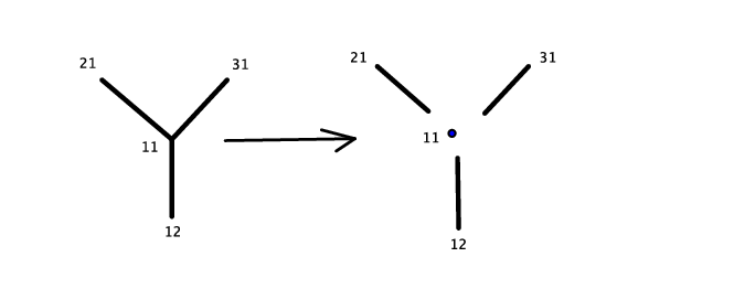
In Figure 1, one can see the process of “exploding” a graph. Notice that we can act on each subgraph by . Compare this to the Weyl-class we obtain:

Lemma 3.
Consider a Weyl-class of graphs representing torus-fixed loci in . For all graphs in the same Weyl-class , the contribution of the Euler class of the normal bundle is the same when specialized to the small torus . That is, for any two graphs in the same Weyl-class
| (19) |
Proof.
The lemma is clear when the formula for is examined. Nontrivial action of on an edge permute homology classes from in the th factor of to the th factor of and thus changes the superscripts in all edge-dependent terms (but not subscripts). (Total degree remains the same.) Similarly, action of on vertices and flags changes super- but not sub-scripts. Specialization to the small torus is geometrically equivalent to taking the quotient of by , and formally equivalent to erasing superscripts. Since action of results only in changes of superscript, it is unseen by the action of . ∎
Similarly, if we let denote the evaluation of insertions at marked points decorating vertices of , we have
Lemma 4.
Consider a Weyl-class of graphs representing torus-fixed loci in . For all graphs ,
| (20) |
Proof.
Insertion is evaluated at the vertex decorated by . A vertex is labelled and the insertion
is evaluated by
Action by on the vertex will permute the (subscripts) but not the (superscripts). is a symmetric polynomial, so specialization to the small torus (erasing superscripts) is invariant under action of . ∎
4. Vanishing of localization contributions
Since specialization from to results in the above-mentioned equalities for and for all in a Weyl-class, we can factor from the sum of localization contributions over each Weyl-class. What remains is the sum of twisting contributions. In this section, we use the notation to denote the twisting contribution of any component of a graph . For , this is the product of evaluation of at vertices of (see equation (18)).
Theorem 3.
The localization contributions of all graphs passing through the diagonal cancel, after specialization of the sum to the small torus .
Proof.
Look at one Weyl-class of graphs passing through the diagonal . (Note that if one graph passes through the diagonal, all graphs in pass through the diagonal and at the same vertices.) “Explode” the graphs by cutting out vertices in the diagonal, leaving finitely many discrete components which we denote by . Each has half-edges where the diagonal was cut away. The contribution of twisting to the localization term can be rewritten
| (21) |
As noted above, for all , , and are the same after specialization. Thus
| (22) |
For , by (18). Vanishing of relies on the fact that has a positive power of as an overall factor (to be proved).
The th component of any exploded graph lies entirely in the good locus . For each graph , label the th component by either or , where and are the two distinct liftings of . Then every graph in is specified by describing, for each , whether the th component is or its opposite, . This is a coin-flipping question – for each component, heads or tails? Thus we can factor the sum of products into a product of sums:
| (23) |
By definition,
Each vertex in corresponds to the vertex in , and after specialization, . Thus
| (24) | ||||
| (25) |
Notice
| (26) |
When is odd, the numerator of this rational expression has no constant term. Thus, is divisible by . What remains is to prove that there are more with odd than the order of the pole, .
In fact, we can do something easier: we can prove that the number of with just one half-edge is greater than . (One half-edge guarantees that is odd.) Let denote the number of components with half-edges. For any graph , . By induction, .
The degree of , then, is greater or equal to
| (27) | ||||
| (28) | ||||
| (29) | ||||
| (30) |
Since because it is enumerative, and appears only for , this quantity is always greater than or equal to 2. Thus we always have a factor of in the sum of localization contributions over a Weyl class whose graphs include a vertex label in the diagonal. Letting shows that the sum of localization contributions over such a Weyl class equals zero. ∎
Combined with Theorem (3), this implies the following:
Theorem 4.
Let be graphs indexing -fixed loci in and let be graphs indexing -fixed loci in . Consider all pairs such that and . Then
5. Further research and extensions
5.1. Case where is greater than 2
Unfortunately, this method becomes combinatorially very complicated for with . In particular, if one sums over Weyl-classes the degree of the pole in the contribution grows factorially with number of edges while the degree of the zero grows linearly. It is possible that a clever use of combinatorics might step around this problem. Currently, though, no method of attack has proved fruitful.
5.2. Higher genus
Higher genus is another situation of interest. Looking at genus zero and , we had
| (31) | ||||
For genus one, we have instead
| (32) | ||||
There is no difference in dimensions of the moduli space, so the twisting bundle has expected dimension zero. For genus greater than one, the expected rank of the twisting bundle is negative. The negativity of rank means that the conjecture does not generalize to higher genus in a straightforward manner.
Acknowledgements
Thanks to Ionuţ Ciocan-Fontanine, my thesis advisor, who suggested this problem and several more. I also benefited from conversation with Ezra Miller, Alexander Voronov, Igor Pak, and Victor Reiner.
References
- [BCFK05] Aaron Bertram, Ionuţ Ciocan-Fontanine, and Bumsig Kim. Two proofs of a conjecture of Hori and Vafa. Duke Math. J., 126(1):101–136, 2005.
- [BCFK08] Aaron Bertram, Ionuţ Ciocan-Fontanine, and Bumsig Kim. Gromov-Witten invariants for abelian and nonabelian quotients. J. Algebraic Geom., 17(2):275–294, 2008.
- [Ber00] Aaron Bertram. Some applications of localization to enumerative problems. Michigan Math. J., 48:65–75, 2000. Dedicated to William Fulton on the occasion of his 60th birthday.
- [CCIT09] Tom Coates, Alessio Corti, Hiroshi Iritani, and Hsian-Hua Tseng. Computing genus-zero twisted Gromov-Witten invariants. Duke Math. J., 147(3):377–438, 2009.
- [CFKS08] Ionuţ Ciocan-Fontanine, Bumsig Kim, and Claude Sabbah. The abelian/nonabelian correspondence and Frobenius manifolds. Invent. Math., 171(2):301–343, 2008.
- [CG07] Tom Coates and Alexander Givental. Quantum Riemann-Roch, Lefschetz and Serre. Ann. of Math. (2), 165(1):15–53, 2007.
- [FP97] W. Fulton and R. Pandharipande. Notes on stable maps and quantum cohomology. In Algebraic geometry—Santa Cruz 1995, volume 62 of Proc. Sympos. Pure Math., pages 45–96. Amer. Math. Soc., Providence, RI, 1997.
- [GP99] T. Graber and R. Pandharipande. Localization of virtual classes. Invent. Math., 135(2):487–518, 1999.
- [Kon95] Maxim Kontsevich. Enumeration of rational curves via torus actions. In The moduli space of curves (Texel Island, 1994), volume 129 of Progr. Math., pages 335–368. Birkhäuser Boston, Boston, MA, 1995.
- [Mar00] Shaun Martin. Symplectic quotients by a nonabelian group and by its maximal torus, 2000.
- [Spi00] Holger Spielberg. The Gromov-Witten invariants of symplectic manifolds, 2000.