Quantum statistics on graphs
Abstract
Quantum statistics, quantum graphs, anyons Quantum graphs are commonly used as models of complex quantum systems, for example molecules, networks of wires, and states of condensed matter. We consider quantum statistics for indistinguishable spinless particles on a graph, concentrating on the simplest case of abelian statistics for two particles. In spite of the fact that graphs are locally one-dimensional, anyon statistics emerge in a generalized form. A given graph may support a family of independent anyon phases associated with topologically inequivalent exchange processes. In addition, for sufficiently complex graphs, there appear new discrete-valued phases. Our analysis is simplified by considering combinatorial rather than metric graphs – equivalently, a many-particle tight-binding model. The results demonstrate that graphs provide an arena in which to study new manifestations of quantum statistics. Possible applications include topological quantum computing, topological insulators, the fractional quantum Hall effect, superconductivity and molecular physics.
1 Introduction
The quantum mechanical properties of a many-particle system depend profoundly on whether the particles are distinguishable or not, even if, in the former case, the distinguishing properties have little effect on the underlying classical mechanics. For this reason, the description of indistinguishable particles in quantum mechanics – quantum statistics – continues to be revisited, both to gain insight into its foundations (Duck & Sudarshan 1997, Berry 2008) as well as to predict and understand new phenomena, including the fractional quantum Hall effect (Wilczek 1990, Jain 2007), superconductivity (Wilczek 1990), topological quantum computing (Nayak et al. 2008) and particle-like states of nonlinear field theories, where standard quantization procedures are not straightforward to apply (Finkelstein & Rubenstein 1968, Manton 2008).
The standard treatment of quantum statistics takes as its starting point the quantum mechanical description of a single particle. The -particle Hilbert space, , is then taken to be the tensor product of copies of the one-particle Hilbert space, . The fact that the particles are indistinguishable means that physically observable operators commute with permutations of the particle labels. This implies that may be decomposed into physically distinct components characterized by different permutation symmetries. The symmetrization postulate restricts the physically realizable spaces to either the symmetric component, which obeys Bose statistics, or the antisymmetric component, which obeys Fermi statistics; components characterized by more complicated behaviour under permutations – parastatistics – are thus excluded. Finally, the spin-statistics relation determines which of the two allowed alternatives applies – Bose statistics for integer spin, and Fermi statistics for half-odd-integer spin.
There is another approach to quantum statistics which is based on the topology of the classical configuration space. It takes as its starting point the configuration space, , of a single particle. The -particle configuration space, , is then taken to be the cartesian product of copies of the one-particle configuration space, with, crucially, coincident configurations excluded (no two particles can be in the same place) and permuted configurations identified. So defined, may have nontrivial topology. In particular, curves along which the particles are exchanged (some particles returning to where they started, others ending up where another started) are regarded as closed curves (as permuted configurations are identified), and these exchange curves cannot be continuously contracted to a single point. If such curves exist, then is multiply connected.
Quantum mechanics on a multiply connected configuration space , whether describes particles or just one, allows for an additional freedom in the quantum description, namely the choice of a representation of the fundamental group, , of . The (single-particle) Aharonov-Bohm effect provides a familiar example: the configuration space for a particle with charge in the presence of an impenetrable solenoid, say along the -axis, may be taken to be with the solenoid – an infinite cylinder – removed. is multiply connected; closed curves may be classified according to the number of times they wind around the excluded cylinder. To the canonical momentum operator, , we can add a vector potential, , whose curl vanishes away from the cylinder, so that the commutation relations are preserved, as are the classical equations of motion – there are no physically accessible magnetic fields. However, the line integral of around the cylinder need not vanish, and may be realized by a magnetic flux inside the cylinder, measured in units of the flux quantum . The flux determines a representation of that assigns to a closed curve with windings the phase factor . The value of the flux modulo – equivalently, the choice of a representation of – affects the quantum mechanical properties, although observable consequences vanish in the classical limit.
More generally, on a multiply-connected configuration space , the momentum is described by a covariant derivative which, in the absence of external fields, has zero curvature (so that the classical mechanics is unaffected) but which may engender nontrivial holonomy. The holonomy corresponds to a representation of the fundamental group . The representation could be one-dimensional and therefore abelian, assigning (commuting) phase factors to noncontractible closed curves, or higher-dimensional, assigning unitary matrices (in general, non-commuting) to noncontractible closed curves. The unitary matrices act on the wavefunctions, which are taken to have components (more generally, wavefunctions are taken to be sections of a -dimensional complex vector bundle).
Taking to be the configuration space of indistinguishable particles, Leinaas and Myrheim (1977) showed that representations of the fundamental group determine the possible realizations of quantum statistics. Similar conclusions were reached by Laidlaw and de Witt (1971) using path integrals, an approach that has been applied in a variety of settings, including cases where canonical quantization is difficult to carry out (Finkelstein and Rubenstein 1968, Balachandran et al. 1993, Manton 2008).
If coincides with the symmetric group, , then the topological approach to quantum statistics yields the same possibilities as does the standard one, namely Bose or Fermi statistics, or, if one gives up the symmetrization postulate, parastatistics, which are associated with higher-dimensional representations of . This is the case for with . As is well known, the situation is different for , i.e. for particles in the plane. The fundamental group is the braid group , which has infinitely many elements. The characterization of unitary representations of the braid group is not complete (see, e.g., Birman & Brendle 2004), but its one-dimensional (abelian) representations include a new type of statistics – anyon statistics (Wilczek 1990). Closed curves on which two of the particles wind around each other times (odd values of correspond to an exchange of positions) are assigned a phase factor , independently of any phases associated with external gauge fields. The special values and correspond to Bose and Fermi statistics respectively.
Anyon statistics have been found to provide deep insight into phenomena involving strongly interacting electrons, for example the fractional quantum Hall effect (Laughlin 1983). In the composite fermion theory (Jain 2007), for example, the collective excitations of the many-electron system are approximately described by an effective Hamiltonian in which they obey anyon statistics with phase related to the fractional Hall conductance.
The situation is different again for , i.e. particles on the line. Here the fundamental group is trivial; there are no noncontractible closed curves, as it is not possible to exchange particles without one passing through another. Thus, the topological approach predicts only Bose statistics (but see Leinaas and Myrheim (1977) for yet another approach to quantum statistics in one dimension).
One motivation for this paper is to study quantum statistics for particles on networks of one-dimensional wires, or metric graphs. A metric graph is a collection of nodes, or vertices, connected by edges, or one-dimensional intervals, of specified lengths. Single-particle quantum mechanics on metric graphs has been extensively studied. The model was originally introduced to describe free electrons on chemical bonds (Pauling 1936). Some current applications include superconductivity (de Gennes 1981), quantum chaos (Kottos and Smilansky 1997, Keating 2008), and Anderson localization (Aizenman et al. 2006). The particle is described by a set of wavefunctions, , one for each edge of . Each wavefunction is acted on by a Hamiltonian, . For example, could be a Schrödinger operator with a gauge potential, i.e. of the form .
The boundary conditions at the vertices of the quantized graph is a subtle point in the theory. For free particles, i.e. , a simple choice motivated by physical considerations is to require that i) wavefunctions are continuous across vertices and ii) the sum of the outgoing derivatives at each vertex should vanish (Neumann-like boundary conditions). A complete characterization of boundary conditions that render the free-particle Hamiltonian self-adjoint has been given in terms of the Lagrangian planes of a certain complex symplectic boundary form (Kostrykin and Schrader 1999, Kuchment 2004). For more general operators, the classification of self-adjoint boundary conditions remains an open problem (see Bolte and Harrison (2003) for a corresponding classification scheme for the Dirac operator). For a given graph model, one can in principle derive physically appropriate boundary conditions from the limiting behaviour of a more realistic two- or three-dimensional model, but the analysis can be quite involved.
As a metric graph is locally one-dimensional, one might imagine that quantum statistics on a metric graph would be limited to Bose or Fermi statistics. This turns out not to be the case, as was previously demonstrated in particular examples by Balachandran & Ercolessi (1992) (discussed in Section 44.4). However, a systematic treatment of quantum statistics for general metric graphs has not been given. One difficulty is that the quantization of many-particle metric graphs poses analytical challenges beyond those encountered in the one-particle theory. Besides boundary conditions for a single particle at a vertex, one has also to specify boundary conditions for coincidences of two or more particles on edges and at vertices that render the many-particle Hamiltonian self-adjoint.
Here we circumvent these difficulties while preserving the essential topological features by considering the simpler problem of indistinguishable particles on a combinatorial graph . A combinatorial graph consists of a set of vertices together with a specification of pairs of vertices that are connected by edges. The edges themselves do not contain any points, so the configuration space for the particle consists of the vertices alone, and hence is zero- rather than one-dimensional. Quantum mechanics on a combinatorial graph is a tight-binding model on the vertices. Thus, quantum statistics on combinatorial graphs is an interesting problem in its own right.
It turns out that the -particle configuration space, , can also be regarded as a combinatorial graph, and hence, in contrast to a many-particle metric graph, is easily quantized. Following the topological approach, we can characterize the possible quantum statistics in terms of representations of the fundamental group of . As is a discrete space, it is not immediately apparent what is meant by its fundamental group, but one can define a combinatorial version that coincides with its metric-graph counterpart.
For simplicity, we consider here two particles on a combinatorial graph, and restrict our attention to abelian (one-dimensional) representations of the fundamental group. It turns out that a given graph may support a family of independent anyon phases associated with topologically inequivalent exchange processes. In addition, for sufficiently complex graphs, there appear new discrete-valued phases. (Mathematically, these discrete phases correspond to representations of the torsion component of the abelianized fundamental group, or, equivalently, the first homology group of .) The results extend straightforwardly to abelian statistics for particles. The extension to nonabelian statistics will be discussed in a forthcoming paper.
The paper is organized as follows. In Section 2 we present quantum mechanics on a combinatorial graph as a tight-binding model. We introduce gauge potentials, the analogue of vector potentials, which assign phase factors to the edges of the graph. These phase factors are then incorporated into the off-diagonal matrix elements (transition amplitudes) of the Hamiltonian matrix. Gauge potentials are determined, up to a choice of gauge, by the accumulated phases along, or fluxes through, the cycles of the graph.
In Section 3 we consider two indistinguishable particles on a combinatorial graph. The two-particle configuration space can itself be regarded as a combinatorial graph (usually larger than the original graph), that can be quantized following the general prescription of Section 2. We characterize, up to a choice of gauge, topological gauge potentials on the two-particle graph, which determine the quantum statistics. Topological gauge potentials have the property that the only cycles with nonzero flux correspond to nontrivial closed curves in the metric setting. They are parameterized by a set of free statistics phases, which range between and , as well as, in some cases, a set of discrete statistics phases whose values are constrained to certain rational multiples of . A certain subset of the free statistics phases may be attributed to Aharonov-Bohm flux lines threading the one-particle graph; the remainder describe many-body effects (Section 33.4). Bose and Fermi statistics, as understood in the conventional approach, may be recovered from particular choices of topological gauge potential (Section 33.5) Our results are illustrated by a number of examples in Section 4, and in the concluding remarks we consider perspectives for further investigations and possible applications.
2 Quantum mechanics on combinatorial graphs
2.1 Combinatorial graphs
A combinatorial graph consists of a set of sites, or vertices, labeled through , which may be connected by bonds, or edges. It is convenient to describe the connectivity of the graph, i.e. its edges, by a adjacency matrix, , whose entry gives the number of edges from vertex to vertex . We assume that is undirected, i.e. . We write to indicate that and are connected by an edge. The number of edges in the graph, , is then given by . Edges will be labeled by Greek indices which take values between and . Given an edge , we let and denote its vertices of lower and higher index respectively. Sometimes it will be useful to assign an orientation to an edge; our convention will be that positive orientation corresponds to going from to .
We also assume that is simple, so that there is at most one edge between any two vertices, and that no vertex is connected to itself, i.e. is equal to zero or one, and is equal to zero. Any graph can be made simple by introducing additional vertices on its multiply-connecting and self-connecting edges. The valency, or degree, , of the vertex is the number of edges connected to , i.e. . Finally, we assume that is connected, i.e. every pair of vertices is connected by some sequence of edges. In terms of the adjacency matrix, this means that, for any given vertices and , for some .
While our focus is on combinatorial graphs, some aspects of our treatment may be motivated by considering metric graphs associated to a combinatorial graph. Given a combinatorial graph, , we can associate to it a metric graph, , by assigning a length to each edge of . On , is regarded as an interval , with identified with and identified with . One can define continuous curves on , and a metric is obtained by taking the distance between two points to be the minimum length of continuous curves joining the points. One can consider closed curves based at a vertex and define the fundamental group in the usual way.
Next we recall some basic facts about the topology of combinatorial graphs (see, e.g., Hatcher 2001), which will play a role in their quantization. A path on a combinatorial graph is a sequence of vertices in which consecutive vertices are connected by edges, i.e. (thus, consecutive vertices must be distinct). The length of a path is the number of edges along it. A single vertex, , may be regarded as a path of zero length, and an edge, , regarded as the path . Given a path , we define the inverse of , denoted , to be the path . If and are two paths such that the last vertex of coincides with the first vertex of , we define the concatenation, or product, of and , denoted , to be the path .
The path describes the product of paths and with an intervening retracing of the path . We want to regard paths that differ by retracings of intermediate components as being the same. Thus, we introduce the equivalence relation . Paths that are equivalent to a zero-length path, i.e. to their initial vertex, are called self-retracing.
A cycle is a path that is closed, i.e. . A cycle is primitive if its vertices, apart from the first and last, are all distinct. The set of cycles on a combinatorial graph can be characterized with the aid of a spanning tree, which we define next. A tree is a combinatorial graph whose only cycles are self-retracing. A subgraph of a combinatorial graph is a combinatorial graph whose vertices and edges are subsets of the vertices and edges of . A spanning tree, , of is a subgraph that is a connected tree containing all the vertices of . Thus, given any two vertices of , there is a path on , unique up to retracings, that joins them. has at least one spanning tree, and, unless is itself a tree, more than one. (An iterative algorithm for constructing a spanning tree is to remove an edge from a primitive cycle of until no primitive cycles remain). Clearly, any spanning tree of has edges. We let denote the number of edges of not in a spanning tree, so is one minus the Euler characteristic of ,
| (1) |
Let denote a spanning tree of and a vertex of . Let us label the edges of that are not in by an index , . Let denote the cycle obtained by proceeding along the (unique) path with no retracings from to on , then from to along , and finally from back to along the (unique) path with no retracings on . We call a fundamental cycle. The definition depends on the choice of and , but the dependence on is easily accounted for, as
| (2) |
where is the (unique) path on from to . An arbitrary cycle beginning and ending at can be expressed, up to retracings, as a product of fundamental cycles and their inverses, i.e.
| (3) |
where . (More formally, the set of cycles based at modulo retracings forms a group, the combinatorial fundamental group . is a free group on generators and is isomorphic to the fundamental group, , of a metric graph, , associated to .)
2.2 Quantization
We regard the set of vertices of a combinatorial graph as a configuration space. might be the configuration space of a single particle, but we shall not restrict ourselves to this point of view. Indeed, in Section 3 we will consider combinatorial graphs whose vertices represent configurations of two particles. We take quantum mechanics on to be given by a tight-binding model on the set of vertices, in which short-time transitions are allowed only between vertices connected by edges. The Hilbert space is , with basis vectors , , describing states in which the system is localized at one of the vertices. Dynamics is given by the Schrödinger equation, , where the Hamiltonian is a hermitian matrix with nonzero off-diagonal entries only between connected vertices, i.e.
| (4) |
One example of a Hamiltonian is (minus) the combinatorial Laplacian, or the discrete kinetic energy, , where is given by .
2.3 Gauge potentials
A gauge potential on is a real antisymmetric matrix such that vanishes if . Given a path on , we define
| (5) |
Clearly, if and differ by retracings, then
| (6) |
and if and can be concatenated, then
| (7) |
For a cycle , we refer to as the flux of through . From (2) and (6), it follows that the flux through a fundamental cycle is independent of ; hence we write , omitting from the notation. For an arbitrary cycle , it follows from (7) that
| (8) |
where and are given by (3). Thus, all fluxes are determined by the fluxes through a set of fundamental cycles.
We incorporate a gauge potential into a Hamiltonian by multiplying the transition amplitudes from to by the phase factors . The new Hamiltonian is given by
| (9) |
Clearly, is hermitian and satisfies (4) (see Oren et al. 2009 for a similar construction).
We can motivate the prescription (9) by making the following analogy with vector potentials on a metric graph. We note that the non-diagonal part of the Hamiltonian can be expressed as a real linear combination of the transition Hamiltonians
| (10) |
where , and, for definiteness, we take . Let denote the edge between and , and consider a metric graph where corresponds to the interval . Let denote the wavefunction along on the quantized metric graph, and let us formally regard and as vertex states localized at and respectively, so that and . Then, formally, , where is the unitary translation by a distance along generated by the momentum operator . Thus we can rewrite (10) as
| (11) |
where denotes the projector . Now suppose we introduce a vector potential on the edge , replacing by , and make the substitution
| (12) |
where is the integral of along . Making this same substitution in (11), we obtain expressions for the transformed transition Hamiltonians, and , that are equivalent to the prescription (9).
A gauge potential is trivial if it is of the form
| (13) |
where is a -tuple of phases and an (antisymmetric) integer matrix. For a trivial gauge potential, is given by , where is the diagonal unitary matrix that generates the gauge transformation . The terminology is in analogy with quantum mechanics on , where a vector potential is trivial if it is a gradient , in which case it is induced by the gauge transformation .
In analogy with the fact that a trivial vector potential has vanishing curl, we have the following characterization of trivial gauge potentials on (we omit the argument, which is not difficult):
| is trivial if and only if is an integer multiple of 2 for every cycle . | (14) |
It follows from (14) and (8) that a gauge potential is determined up to a gauge transformation by its fluxes through a set of fundamental cycles. Indeed, given a set of fluxes , we can construct a gauge potential for which , as follows: if and are vertices of an edge in , we take
| (15) |
For an edge not in with vertices and , we take
| (16) |
3 Two particles
3.1 Quantization
Given a one-particle configuration space, , there is a standard construction for the configuration space, , of two indistinguishable particles on (the construction generalizes straightforwardly to more than two particles). consists of unordered pairs of distinct points of , i.e.
| (17) |
where denotes the coincident two-particle configurations, which are excluded, and denotes the symmetric group, whose single nontrivial element – exchange – acts on according to .
Given a combinatorial graph , we shall now regard the set of its vertices, , as a one-particle configuration space. Hence, we take to be the configuration space for two indistinguishable particles on . Depending on context, we denote configurations in either by unordered pairs of vertices , or by ordered pairs with .
We may regard as a new combinatorial graph. Nodes (or -vertices) and are taken to be connected by an edge if they have one -vertex in common while their other -vertices are connected by an edge of . Equivalently, moving along an edge of corresponds to keeping one particle fixed at a vertex of while moving the other along an edge of . The adjacency matrix of , denoted , is given by
| (18) |
where is the adjacency matrix of . (To avoid awkward notation, we will not relabel the vertices of by a single index.) The number of vertices and edges of , denoted and respectively, are given by
| (19) |
We define quantum mechanics on following the prescription of Section 22.2. The Hilbert space is with basis vectors , , representing states where one particle is at site and the other at site . Two-particle Hamiltonians, denoted , are -dimensional hermitian matrices , where and , whose off-diagonal elements, i.e., elements for which , vanish whenever vanishes. Thus, short-time transitions generated by involve one particle making an allowed transition on while the other particle remains fixed.
Given a one-particle Hamiltonian on , we can construct a two-particle Hamiltonian on according to
| (20) |
where (one can check that satisfies (4)). As discussed in Section 33.5 below, describes noninteracting fermions, while describes hard-core (and therefore interacting) bosons which are prevented from occupying the same site. A simple illustration (two free particles on a linear graph) is given in Section 44.1.
3.2 Topological gauge potentials
Gauge potentials can be introduced on a two-particle combinatorial graph following the general prescription of Section 22.3. Quantum statistics is described by a subset of these, which we call topological gauge potentials. As discussed below, topological gauge potentials correspond to gauge potentials on a two-particle metric graph whose fluxes through all contractible closed curves vanish (modulo ). Thus, their effects are purely quantum mechanical, vanishing in the classical limit.
Let be a combinatorial graph, and the corresponding two-particle combinatorial graph. Let and denote disjoint edges of , i.e. and have no vertices in common. Let denote the cycle on given by
| (21) |
That is, along , the particles move in alternating steps back and forth along and . We say that is metrically contractible. The reason is that corresponds to a loop on , the two-particle configuration space for a metric graph associated with , which can be continuously contracted to a point – see Figure 1.
(These considerations may be made more formal. Let denote a vertex of the two-particle configuration space. One can show that is isomorphic to the quotient of by the subgroup generated by cycles of the form , where and are disjoint and is a path from to .)
Let denote a gauge potential on . We say that is a topological gauge potential if its flux through every metrically contractible cycle vanishes modulo , i.e.
| (22) |
(More formally, topological gauge potentials may be identified with one-dimensional representations of .)
Informally, gauge potentials that are not topological may be understood to introduce additional forces into the underlying classical dynamics, as the following heuristic argument, based on the analogy with metric graphs, demonstrates: when one particle is on the edge and the other on , the free-particle Hamiltonian for the two-particle metric graph is given by . If we introduce a gauge potential, replacing by and by , the equations of motion become
| (23) |
where the gauge field, , is given by . If (analogous to , the classical motion is no longer free. For combinatorial graphs, some numerical evidence for the effects of these gauge forces is given in Section 44.1.
3.3 Characterization of topological gauge potentials
Given a combinatorial graph , we obtain below an explicit parametrization of the topological gauge potentials on the two-particle graph, . The parametrization is given in terms of a set of fluxes, or phases.
Let denote a spanning tree of . As shown in Section 22.3, given a gauge potential on (not necessarily topological), we can choose a gauge so that vanishes on the edges of . Let us label the edges of that are not in by an index , and let denote the corresponding fundamental cycles. The number of such cycles, which we denote by , is given by (cf. (1))
| (24) |
Let denote the flux of through . Then is determined by .
The conditions on topological gauge potentials (cf. (22)) can be expressed as linear relations on the components of . It will be convenient to label pairs of disjoint edges by a single index . The number of such pairs, which we denote by , is just the difference between the number of all pairs of edges of and the number of pairs of edges that share a vertex, so that
| (25) |
Therefore, the condition for to be a topological gauge potential can be written as
| (26) |
where is a integer matrix and an arbitrary -dimensional integer vector. The specific form of depends on the choice of fundamental cycles. We note that the rows of may be linearly dependent (this turns out to be the case if, for example, contains two or more disjoint cycles).
The system (26) can be solved by expressing in Smith normal form (see, e.g., Dummit & Foote 2003). We write
| (27) |
where and are integer matrices with integer inverses of dimensions and respectively, and is a nonnegative diagonal integer matrix. The number of nonzero diagonal elements of is given by the rank of , denoted , and may be chosen so that its first diagonal elements are nonzero with divisible by for . The nonzero diagonal elements of are called the divisors of . They are uniquely determined by , and do not depend on the choice of fundamental cycles (i.e., they are basis-independent).
Substituting the Smith normal form (27) into (26), we can write the conditions on as
| (28) |
where is integral and . may be regarded as the flux of through a cycle in which the fundamental cycle appears with multiplicity given by .
From (28), the allowed values of depend on , and in particular on whether is one, greater than one, or zero. Let denote the number of divisors of equal to one, the number of divisors greater than one, and the number of vanishing diagonal elements of . Then (28) can be written as
| (29) |
where is shortened notation for the divisors of greater than one. Once the ’s are specified, , and hence , are determined by .
Thus, topological gauge potentials are parameterized by phases taking values between and , and phases taking values constrained to be rational multiples of . We shall refer to the ’s as free statistics phases and the ’s as discrete statistics phases. Examples of both are given in Section 4. (More formally, the set of topological vector potentials modulo trivial gauge potentials, regarded as a group under matrix addition modulo , is isomorphic to , and is the character group of .)
3.4 Aharonov-Bohm phases and two-body phases
Among the free statistics phases, there may be some that correspond to one of the particles going around a cycle on while the other remains fixed. Physically, such phases could be produced by solenoids threading the cycles of with magnetic flux (assuming the particles are charged). From the point of view of quantum statistics, we would like to distinguish between contributions to topological gauge potentials that may be attributed to individual particles interacting with an external gauge potential, on the one hand, and contributions involving many-body effects on the other.
Let be a gauge potential on a combinatorial graph . We can construct a corresponding gauge potential on , denoted , following the prescription (20) for constructing a two-particle Hamiltonian from a single-particle Hamiltonian, i.e.
| (30) |
is antisymmetric (since is antisymmetric), and hence constitutes a gauge potential on . We shall call gauge potentials of the form (30) Aharonov-Bohm potentials. They are parameterized (up to a choice of gauge) by fluxes, or Aharonov-Bohm phases, , through a set of fundamental cycles on .
Given a cycle on , the flux can be evaluated as follows. Let and denote the paths on described by the individual particles as is traversed. If each particle returns to where it started, then and are themselves cycles, and we say that is a direct cycle. In this case, is the sum of one-particle fluxes, i.e.
| (31) |
Note that (31) implies that is in fact a topological gauge potential; and are self-retracing cycles on the edges and through which the flux of obviously vanishes. If is not a direct cycle, then the particles exchange positions along , and we say that is an exchange cycle. In this case, the last vertex of is the first vertex of , and vice versa, and
| (32) |
We will say that two topological gauge potentials and are AB-equivalent if their difference, , is an Aharonov-Bohm potential; equivalently, can be produced from by adjusting the Aharonov-Bohm fluxes . We would like to find parameters that determine topological gauge potentials up to AB equivalence. These parameters, together with the ’s, then provide a complete parametrization of topological gauge potentials (up to a choice of gauge).
We proceed by fixing a representative from each family of AB-equivalent topological gauge potentials, and then finding parameters that characterize . For the special case of circular graphs this is easily done. Circular graphs have their vertices arranged on a ring, and the only edges are between adjacent vertices. We may take , because every topological gauge potential may be generated by an Aharonov-Bohm flux through the ring. Circular graphs are discussed further in Section 44.2.
Assuming that is not a circular graph, we can choose a set of fundamental cycles on such that none of the ’s contains every vertex of . Let denote a vertex of not contained in , and let denote the cycle on on which one particle traverses while the other remains fixed at . We fix (up to a choice of gauge) by requiring that
| (33) |
(a straightforward argument shows that every topological gauge potential is -equivalent to a unique topological gauge potential satisfying (33)).
The linear conditions (33) on can be combined with the linear conditions (22) which characterize general topological vector potentials, and the two sets of conditions written collectively as (cf. (26))
| (34) |
where is an integer matrix of dimension , and is an integer vector of dimension . The solution of (34) proceeds as in Section 33.3. Solutions are parameterized by phases , which we call two-body phases, and discrete statistics phases . It follows that a general topological gauge potential may be parameterized by Aharonov-Bohm phases , which determine its fluxes through the ’s, in addition to the two-body phases and discrete statistics phases . The lasso and bowtie graphs (Section 44.4) provide simple illustrations of the distinction between Aharonov-Bohm and two-body phases.
3.5 Bose and Fermi statistics
Our treatment of quantum statistics on combinatorial graphs – referred to in what follows as the identified scheme – follows the approach of Leinaas and Myrheim (1977), treating the particles as classically indistinguishable. If instead one followed the conventional approach – referred to in what follows as the distinguished scheme, in which the particles are labeled from the start, one would find Bose and Fermi statistics. Below we establish the relationship between the two schemes. Note that, in the identified scheme, it does not make sense to speak of the exchange symmetry of a quantum state, as exchange is not defined – the wavefunction assumes a single value for each configuration of the indistinguishable particles. It turns out that Bose and Fermi statistics may be regarded as particular cases of the more general quantum statistics we have obtained here. In particular, Bose statistics corresponds to a trivial (e.g., vanishing) topological gauge potential, while Fermi statistics corresponds to a topological gauge potential that assigns a phase of to exchange cycles and zero phase to direct cycles.
Following the distinguished scheme one proceeds as follows. Let denote a combinatorial graph with adjacency matrix . We introduce the distinguished two-particle configuration space, denoted , or for short, that consists of ordered pairs , , of distinct vertices of (note that particles are still not allowed to occupy the same vertex). We regard as a graph with vertices and adjacency matrix
| (35) |
Following the general quantization prescription given in Section 22.2, we introduce the distinguished Hilbert space , with basis vectors , , which describe states where particle 1 is at vertex and particle 2 at vertex . A quantum Hamiltonian on , denoted , is a -dimensional matrix with matrix elements
| (36) |
satisfying (4) (so that short-time transitions are single-particle transitions).
Exchange is defined on by . We decompose into two -dimensional subspaces, , consisting of states that are even () or odd () under exchange. Indistinguishability is incorporated by requiring the Hamiltonian (and, indeed, any hermitian matrix representing an observable) to be invariant under exchange, i.e. . Then preserves exchange symmetry, i.e. it leaves the subspaces invariant.
For example, given a one-particle Hamiltonian , we may construct the two-particle Hamiltonian
| (37) |
On the antisymmetric subspace , the energy levels of are just sums of distinct energy levels of , and the two-particle eigenstates are antisymmetric products of one-particle eigenstates – this corresponds to noninteracting fermions. The situation is different on the symmetric subspace . In general, the spectrum of on is not simply related to the one-particle spectrum (although in some special cases it is). This is because the diagonal states are excluded; bosons are prevented from occupying the same vertex, which, unlike fermions, they would otherwise do.
The equivalence between the identified and distinguished schemes may be established by means of a unitary map, , from the identified Hilbert space, , to the symmetric or antisymmetric subspace, , of the distinguished Hilbert space. is given by
| (38) |
Given an exchange-invariant Hamiltonian on , we can construct a unitarily equivalent Hamiltonian on by taking . The matrix elements of are given explicitly by
| (39) |
Thus, in the identified scheme, the statistics sign appears in the Hamiltonian , while the Hilbert space, , is independent of . In contrast, in the distinguished scheme, determines the Hilbert space , while the Hamiltonian is independent of . In particular, if is given by the sum of one-particle Hamiltonians as in (37), then (39) yields
| (40) |
This is in accord with (20), and establishes that corresponds to Bose or Fermi statistics.
From (39) and the constraints (4), we can express the relation between the Bose and Fermi Hamiltonians and as
| (41) |
where is given by
| (42) |
Thus, and are related by a gauge potential, as is real antisymmetric and its th element vanishes unless . In fact, is a topological gauge potential. This can be verified by checking the conditions (22) explicitly. Alternatively, we may argue as follows: given a path on of length , let and denote the single-particle paths along . Nonzero contributions of to come from those edges of where the ordering of the single-particle positions switches over, either from to or from to . However, on a direct cycle , and, in particular, on , the particles separately return to where they started, so the number of switchovers, and hence the number of contributions, must be even – therefore is a multiple of . Indeed, by this reasoning we see that
| (43) |
4 Examples
We investigate statistics phases for a number of graphs, starting with the simplest examples.
4.1 Linear graphs
The linear graph consists of vertices on a line with adjacent vertices connected by edges, so that . From the point of view of quantum statistics, linear graphs are trivial; it turns out that there are no nontrivial topological gauge potentials on two-particle linear graphs. However, linear graphs provide simple examples where the free-particle energy levels and eigenstates can be calculated explicitly, and they serve to illustrate some points of the preceding discussion, including the equivalence of Bose and Fermi statistics in cases where topological phases are absent, as well as the effect of non-topological gauge potentials.
Let be the one-particle kinetic energy on (cf. Section 22.2. It is straightforward to show that the energy levels of are given by , , while the eigenstates are given, up to normalization, by . We take the two-particle Hamiltonian, , to be the sum of one-particle Hamiltonians as given by (20). As discussed in Section 33.5, corresponds to Bose statistics and to Fermi statistics. It is straightforward to show that the energy levels of are independent of , and are given by sums with and distinct. The corresponding eigenstates are, for , antisymmetric products of distinct eigenstates and , and, for , symmetric products of these eigenstates with diagonal components removed. The interaction between the (hard-core) bosons is reflected in the fact that two-particle states with are absent from the spectrum.
The fact that the Bose and Fermi spectra coincide for linear graphs can be understood from our topological treatment of quantum statistics. The only nontrivial cycles on the two-particle configuration space correspond to each particle moving back and forth in alternation along separated segments of the linear graph. Such cycles are metrically contractible, so that there are no nontrivial topological gauge potentials. It follows that Fermi gauge potential (cf. (42)) is just a gauge transformation.
There is an alternative, single-particle interpretation of , namely as a discrete approximation to the quantum Hamiltonian for a free particle in a two-dimensional right triangular domain with sides , and (i.e., half the unit square below the diagonal), and with . Neumann boundary conditions apply on the right sides of the triangle, while determines the boundary condition on the diagonal (Neumann for , Dirichlet for ).
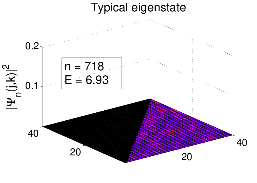
Fixing the Hamiltonian to be for definiteness, it is instructive to observe the consequences of introducing a gauge potential, denoted , that is not topological. Let us take to have flux through every cycle where is an edge between vertices in the range between and , and an edge between vertices in the range between and . For cycles outside this range, we take . In terms of the single-particle interpretation, corresponds to a uniform magnetic field of strength (in units where , being the charge of the particle, is equal to one) through the square of area with diagonal corners and . Numerical calculations show that the shifts in energy levels produced by scale with , in accord with the fact that a magnetic field does not change the mean density of states. However, with present, while typical eigenstates are delocalized (cf. Figure 2), one finds some eigenstates that are strongly localized in the flux square and (cf. Figure 2). In the single-particle interpretation these are Landau-like levels, and are indicative of Lorentz forces in the classical dynamics.

4.2 Circular graphs
The circular graph, , is obtained by connecting the first and last vertices of the linear graph . For a circular graph, we naturally expect, and indeed find, anyon statistics, confirming that our model provides a reasonable description of quantum mechanics on a loop. For simplicity we consider a loop with three vertices, shown in Figure 3 (a) (the conclusions are similar for ). Writing down the three allowed two-particle configurations in Figure 3 (b), it is apparent that the two-particle graph is also a single loop. A single traversal of this loop is an exchange cycle, and the associated flux corresponds to anyon statistics. The flux can be generated by an Aharonov-Bohm potential, corresponding to a solenoid threading the one-particle graph .
4.3 Star graphs
The star graph, , shown in Figure 4 (c), consists of vertices each connected to a central vertex, and so has edges and vertices. We consider first the star graph, or -graph, for which the two-particle graph is easily displayed (Figures 4 (a) and (b)). The two-particle graph consists of a single cycle which exchanges the particles through the arms of the ‘Y’. A flux through this cycle produces anyon statistics. For , the two-particle star graph consists of vertices and edges. The number of independent cycles, , is given by . There are no Aharonov-Bohm phases (there are no nontrivial cycles on ) and no constraints on topological gauge potentials (there are no disjoint edges on ). Therefore, topological gauge potentials on are parameterized by two-body statistics phases. The number of statistics phases can also be obtained from the following simple argument: each phase corresponds to the choice of a pair of edges along which to exchange the particles, given that the particles start on the vertices of some given edge. is therefore the number of pairs of objects.
4.4 Lasso and bowtie
The lasso graph consists of a three-vertex loop with a single external lead – see Figure 5 (a). It provides a simple example of quantum statistics which combines aspects of circular graphs and star graphs discussed above. The two-particle lasso, , is shown Figure 5 (b) along with a spanning tree, (in bold). We fix the gauge so that the edges of are assigned zero phase. The three edges of not in determine the fundamental cycles. The central square corresponds to the metrically contractible cycle on which the particles move in alternation along the edges and of the lasso. As the flux through this cycle must vanish, the edge is assigned zero phase as well. The left triangle of corresponds to the cycle in which the one of the particles goes around the loop of the lasso while the other remains on the external lead, and may be assigned an Aharonov-Bohm phase . The right triangle of corresponds to an exchange cycle in which the particles move around the loop of the lasso. The associated phase, denoted , is a two-body phase. The length-six cycle along the perimeter of coincides with the exchange cycle on the graph, and has phase . These results coincide with those of Balachandran & Ercolessi (1992), who considered the two-particle metric lasso graph.
Another example considered by Balachandran & Ercolessi (1992) is the bowtie, or figure-of-eight, which consists of two three-vertex loops sharing a common vertex – see Figure 5 (c). Calculations show that the two-particle bowtie has two Aharonov-Bohm phases (corresponding to the two loops) and two two-body phases.
4.5 Nonplanar graphs: , and the molecule
is the fully connected graph with five vertices, and is the fully connected bi-partite graph with two sets of three vertices – see Figure 6 (a) and (b). A theorem of Kuratowski (1930) states that every non-planar graph (i.e., a graph that cannot be drawn in the plane without crossings) contains or as a subgraph (possibly after contracting some edges to points). From the point of view of quantum statistics, and are interesting because they are the smallest graphs that exhibit discrete statistics phases. Calculations following the procedure of Section 33.3 (details are omitted) show that has six Aharonov-Bohm phases and has four Aharonov-Bohm phases (corresponding to their respective number of fundamental cycles). In addition, both have a single discrete statistics phase that can be either or (mod ). Cycles whose fluxes are given by this discrete phase are necessarily exchange cycles. An example for consists of the cycle in which one particle goes around a three-vertex loop (e.g., ) while the other remains fixed, followed by an exchange around the same three-vertex loop in the opposite direction (e.g., ). An example for consists of the cycle in which one particle goes around a four-vertex bowtie loop (e.g., ) while the other remains fixed, followed by an exchange around the same four-vertex loop in the opposite direction (e.g., ).
The molecule is the graph consisting of two ’s joined by a single edge, as in Figure 6 (c). Calculations (again, details are omitted) show that two discrete statistics phases appear, both either or , along with 12 Aharonov-Bohm phases and 6 two-body phases.
5 Discussion
The abelian statistics of two indistinguishable quantum particles on a combinatorial graph are characterized by a set of continuous and discrete-valued phases. The continuous phases may be separated into some that are produced by external Aharonov-Bohm fluxes and the rest describing two-body statistical interactions. The appearance of discrete phases may be related to whether the graph is planar or not, a connection that merits further investigation. While we have concentrated on the case of two particles, the abelian statistics for more than two particles may be characterized and calculated using the results presented here.
Nonabelian statistics requires new considerations. A full description is needed of the fundamental group of the -particle configuration space, or, equivalently, the braid groups of the graph (not simply their abelianized versions). Recently, Farley & Sabalka (2005) have developed methods based on discrete Morse theory for obtaining efficient presentations of graph braid groups. We will discuss applications of these techniques to nonabelian graph statistics in a forthcoming publication (see (Kitaev 2008) for an exact solution of a spin-lattice model where nonabelian statistics emerge).
From the point of view of physics, one of the principal attractions of quantum graphs is that they provide mathematically tractable models of complex physical systems. As applications have so far concentrated on independent-particle models, the scope for manifestations of quantum statistics on graphs is great. We suggest a few possibilities here. Graph statistics may play a role in many-electron network models of molecules, in analogy with the emergence of the Berry phase – the molecular Aharonov-Bohm effect (Mead and Truhlar 1979) – in molecular spectra. Topological signatures in single-particle transport on networks (Avron 1995), which provide models and variants of the quantum Hall effect, may have many-particle generalizations in which statistics plays a role. Many-particle graphs may provide new models for anyon superconductivity (Wilczek 1990). An intriguing potential application of nonabelian graph statistics is to topological quantum computing (Nayak et al. 2008). There one looks for systems with a degenerate ground state spanned by distinct quasiparticle configurations, in which the only (easily) realizable evolutions are, up to a phase, a discrete set of unitary transformations generated by the (adiabatic) exchange of quasiparticles. By introducing spin (Harrison 2008), quantum graphs might also provide models in which to investigate the role of quantum statistics in the quantum spin Hall effect and topological insulators (Hasan & Kane 2010, Qi & Zheng 2010).
Applications will depend on nontrivial graph statistics emerging
in a particular model. A standard approach would be to look for
novel many-particle ground states on graphs and to study their
excitations. This is work for the future. However, even without a
specific mechanism, we believe it is worthwhile to pursue a
general investigation of
quantum statistics on networks and its
consequences. Quantum physics has provided many examples where
topology underlies new and unexpected phenomena. Nature seems to
exploit the opportunities available to it, and discoveries may
follow from knowing where to look and what to look for.
Acknowledgements. We thank Dan Farley for helpful discussions. JMH is supported by National Science Foundation grant DMS-0604859.
References
- [1] Aizenman, M., Sims, R. & Warzel, S. 2006 Commun. Math. Phys. 264, 371–389.
- [2] Avron, J.E. 1995 Adiabatic quantum transport. In Mesoscopic Quantum Physics (Les Houches Summer School Proceedings). Amsterdam: Elsevier. eds. E. Akkermans, G. Montambaux and J.L. Pichard North-Holland
- [3] Balachandran, A.P. & Ercolessi, E. 1992 Int. J. Mod. Phys. A7, 4633–4654.
- [4] Balachandran, A.P., Daughton, A., Gu, Z., Marmo, G., Sorkin, R.D., & Srivastava, A.M. 1993 Int. J. Mod. Phys. A8, 2993–3044.
- [5] Berry, M.V. 2008. Nonlinearity 21, T19–T26.
- [6] Birman J.S. & Brendle, T.E. 2005 Braids: A survey. In Handbook of Knot Theory (eds. W. Menasco & M. Thistlethwaite). Amsterdam: Elsevier.
- [7] Bolte, J. & Harrison, J.M. 2003 J. Phys. A 36 L433–L440.
- [8] Duck, I. & Sudarshan, E.C.G. 1997 Pauli and the spin-statistics theorem. Singapore: World Scientific.
- [9] Dummit, D.S. & Foote, R.M. 2003 Abstract algebra, 3rd edn. Wiley.
- [10] Farley, D. & Sabalka, L. 2005 Algebr. Geom. Topol. 5, 1075-1109.
- [11] Finkelstein, D. & Rubenstein, J. 1968 J. Math. Phys. 9, 1762–1779.
- [12] de Gennes, P.G. 1981 C. R. Acad. Sci. Paris 292 279–282.
- [13] Harrison, J.M. 2008 Quantum graphs with spin Hamiltonians. In Analysis on graphs and its applications (eds. P. Exner, J. P. Keating, P. Kuchment, T. Sunada, A. Teplyaev) Proceedings of Symposia in Pure Mathematics 77 AMS, 261–277.
- [14] Hasan, M.Z. & Kane, C.L. 2010, arXiv:1002.3895v1 [cond-mat.mes-hall].
- [15] Hatcher, A. 2001 Algebraic topology. Cambridge: Cambridge University Press.
- [16] Jain, J.K. 2007 Composite fermions. Cambridge: Cambridge University Press.
- [17] Keating, J.P. 2008 Quantum graphs and quantum chaos. In Analysis on graphs and its applications (eds. P. Exner, J. P. Keating, P. Kuchment, T. Sunada, A. Teplyaev) Proceedings of Symposia in Pure Mathematics 77 AMS, 261–277.
- [18] Kitaev, A. 2006 Ann. Phys. 321, 2–111; arXiv:cond-mat/0506438v3.
- [19] Kostrykin, V. & Schrader, R. 1999 J. Phys. A 32, 595–630.
- [20] Kottos, T. & Smilansky, U. 1997 Phys. Rev. Lett. 79, 4794–4797.
- [21] Kuchment, P. 2004 Waves Random Media 14, S107–128.
- [22] Kuratowski, K. 1930 Fund. Math. 15, 271–283.
- [23] Laidlaw, M.G.G. & DeWitt, C.M. 1971 Phys. Rev. D 3, 1375-1378.
- [24] Laughlin, R. B. 1983. Phys. Rev. Lett. 50, 1395–1398.
- [25] Leinaas, J.M. & Myrheim, J. 1977 Nuovo Cim. 37B, 1–23.
- [26] Manton, N.S. 2008 Nonlinearity 21, T221-T232.
- [27] Mead, C.A. & Truhlar, D.G.J. 1979. Chem. Phys. 70, 2284-2296.
- [28] Nayak, C., Simon, S.H., Stern, A., Freedman, M., & Das Sarma, S. 2008. Rev. Mod. Phys. 80, 1083–1159.
- [29] Oren, O., Godel, A. & Smilansky, U. 2009 J. Phys. A 42, 415101.
- [30] Pauling, L. 1936 J. Chem. Phys. 4, 673–677.
- [31] Qi, X.L. & Zheng, S.C. 2010. Phys. Today 63, 33–38.
- [32] Wilczek, F. (ed) 1990 Fractional statistics and anyon superconductivity. Singapore: World Scientific.