A Floer-Gysin exact sequence for Lagrangian submanifolds

1. Introduction and main results

This paper is concerned with a Floer-theoretic analogue of the well known Gysin-sequence from algebraic topology. In this paper we focus on the case of circle bundles only. Recall that given a circle bundle $\pi:\Gamma^{n+1}\longrightarrow L^{n}$ over a closed manifold $L$ there is a long exact sequence in cohomology:

\begin{CD}\cdots @>{}>{}>H^{k}(L)@>{\cup\,e}>{}>H^{k+2}(L)@>{\pi^{*}}>{}>H^{k+2}(\Gamma)@>{\pi_{*}}>{}>H^{k+1}(L)@>{}>{}>\cdots\end{CD}

where $e\in H^{2}(L)$ is the Euler class of the circle bundle and $\pi_{*}:H^{*+1}(\Gamma)\longrightarrow H^{*}(L)$ is the map that can be identified under Poincaré duality with the map induced by the projection $H_{n-*}(\Gamma)\longrightarrow H_{n-*}(L)$ (sometimes the map $\pi_{*}$ is also called “integration along the fibres”).

In this paper we will develop a Floer analogue of this sequence associated to a Lagrangian submanifold $L$ and certain circle bundle over it that appears naturally in certain geometric circumstances.

Let $(\Sigma,\omega_{\Sigma})$ be a closed symplectic manifold with an integral symplectic structure, i.e. $[\omega_{\Sigma}]\in H^{2}(\Sigma;\mathbb{R})$ admits a lift to $H^{2}(\Sigma;\mathbb{Z})$ . Let $L\subset\Sigma$ be a Lagrangian submanifold. One of the motives of this paper is to study the Floer cohomology of $L$ and derive from it possible applications, e.g. to questions concerning the topology of $L$ .

Our starting point is that one can associate to $L$ in a natural way a flat circle bundle $\Gamma_{L}\to L$ whose total space $\Gamma_{L}$ can be realized as a Lagrangian submanifold in a new symplectic manifold which is a bundle over $\Sigma$ . The construction is simple. Fix a lift $a\in H^{2}(\Sigma;\mathbb{Z})$ of $[\omega_{\Sigma}]$ and let $\mathcal{N}\to\Sigma$ be the complex line bundle with $c_{1}^{\mathcal{N}}=a$ . One can endow $\mathcal{N}$ with a hermitian metric and a connection so that the curvature of $\mathcal{N}$ is $\tfrac{i}{2\pi}\omega_{\Sigma}$ . The total space of $\mathcal{N}$ can be endowed with a canonical symplectic structure $\omega_{\textnormal{can}}$ which restricts to $\omega_{\Sigma}$ on $\Sigma$ . Fix $r_{0}>0$ and let $P_{r_{0}}\subset\mathcal{N}$ be the circle bundle of radius $r_{0}$ and denote by $\pi:P_{r_{0}}\to\Sigma$ the projection. Then $\Gamma_{L}=\pi^{-1}(L)$ becomes a Lagrangian submanifold of $(\mathcal{N},\omega_{\textnormal{can}})$ . Note that $\Gamma_{L}$ in fact lies in $\mathcal{N}\setminus\Sigma$ .

Ideally one would like to relate the symplectic topology of $L\subset\Sigma$ to that of $\Gamma_{L}\subset\mathcal{N}$ or that of $\Gamma_{L}\subset\mathcal{N}\setminus\Sigma$ , hoping that the latter would shed some new light on $L$ . The problem is that both $\mathcal{N}$ and $\mathcal{N}\setminus\Sigma$ have a symplectically concave end (at infinity) which apriori makes them inaccessible to the current techniques of symplectic topology, in particular Floer theory. Nevertheless, we will see that one can still define a version of Floer cohomology for $\Gamma_{L}\subset\mathcal{N}\setminus\Sigma$ . Moreover, we will see that the Floer cohomology of $L$ and that of $\Gamma_{L}$ are related by a long exact sequence which is analogous to the Gysin sequence relating the singular cohomologies of $L$ and $\Gamma_{L}$ .

Although we can define the Floer cohomology for $\Gamma_{L}\subset\mathcal{N}\setminus\Sigma$ this notion is apriori not very useful unless we can establish some geometric properties of this cohomology, such as invariance under Hamiltonian isotopies, a vanishing criterion when $\Gamma_{L}$ is displaceable etc. This is not so clear in general since the manifold $\mathcal{N}\setminus\Sigma$ has a concave end. However, there is one situation in which one can go through these difficulties: when the contact manifold $P_{r_{0}}$ is Weinstein fillable. This means that $\mathcal{N}\setminus\Sigma$ (which is just the negative symplectization of $P_{r_{0}}$ ) can be compactified at the negative (or concave) end into a Weinstein manifold $W$ . As we will see later the Floer cohomology of $\Gamma_{L}$ in $\mathcal{N}\setminus\Sigma$ coincides with that of $\Gamma_{L}$ in $W$ . The latter is already a completely standard object in symplectic topology and enjoys the usual geometric properties expected from the theory. The fundamental example of fillable $P_{r_{0}}$ is when $\Sigma$ appears as a symplectic hyperplane section in closed symplectic manifold $M$ (of one complex dimension higher). Then $W=M\setminus\Sigma$ is Weinstein and if one removes from it the isotropic skeleton $\Delta\subset W$ we have $W\setminus\Delta\approx\mathcal{N}\setminus\Sigma$ . In view of this we will from now on work in this geometric framework. Here is the setup.

Let $(M,\omega)$ be a symplectic manifold with an integral symplectic structure, i.e. $[\omega]\in H^{2}(M;\mathbb{Z})$ . Let $\Sigma\subset M$ be a symplectic hyperplane section of degree $k$ , so that $PD[\Sigma]=k[\omega]$ (see [Don]). In this setup, the Lagrangian circle bundle construction [Bir2, BC2] associates to every Lagrangian submanifold $L\subset\Sigma$ a new Lagrangian submanifold $\Gamma_{L}\subset M\setminus\Sigma$ which topologically is a circle bundle over $L$ . The construction of $\Gamma_{L}$ is roughly the following (see §2 and more specifically §2.4 for the precise details). Take a tubular neighborhood $\mathcal{U}$ of $\Sigma$ in $M$ which looks like a disk bundle over $\Sigma$ , say $\mathcal{U}\to\Sigma$ . Its boundary $P=\partial\mathcal{U}$ is a circle bundle $\pi:P\to\Sigma$ over $\Sigma$ . Define

\Gamma_{L}=\pi^{-1}(L)\subset M\setminus\Sigma.

For an appropriate choice of the neighborhood $\mathcal{U}$ the resulting $\Gamma_{L}$ will be a Lagrangian submanifold of $M\setminus\Sigma$ . This procedure, which was introduced in [Bir2, BC2], proved to be useful for studying Lagrangians in manifolds $\Sigma$ that appear as hyperplane sections (in some manifold $M$ ). The point is that the symplectic topology of $M\setminus\Sigma$ is sometimes easier to study than that of $\Sigma$ itself.

As $\Gamma_{L}\to L$ is a circle bundle the singular cohomologies of the manifolds $\Gamma_{L}$ and $L$ are related by the Gysin long exact sequence. As we will see soon, there is an analogous long exact sequence relating their Floer cohomologies too.

Before we state our main theorem we need to introduce some notation and elaborate more about the setting. Given a symplectic hyperplane section $\Sigma\subset M$ , put $W=M\setminus\Sigma$ . We will assume from now on that $W$ is a Weinstein manifold. (This is often assumed as part of the definition of “symplectic hyperplane section”.) The basic familiar example is when $M$ is Kähler and $\Sigma$ is a complex hyperplane section (then $W$ is in fact affine). As for the Lagrangian $L\subset\Sigma$ we will henceforth assume that it is monotone with minimal Maslov number $N_{L}\geq 2$ (see e.g. [BC6] for the definition). In what follows we will mostly work with $\mathbb{Z}_{2}$ as the ground field both for Floer cohomology as well as for singular cohomology. In particular when we refer to the Euler class $e$ of the circle bundle $\Gamma_{L}\to L$ we actually mean the $\mathbb{Z}_{2}$ -reduction of the integral Euler class, so that $e\in H^{2}(L;\mathbb{Z}_{2})$ .

We denote by $HF^{*}(L)$ the Floer cohomology of the pair $(L,L)$ . Since $L$ is monotone the coefficient ring will be taken to be the ring of Laurent polynomials $\Lambda=\mathbb{Z}_{2}[t^{-1},t]$ where $\deg t=N_{L}$ (see e.g. [BC6]). Similarly we denote by $HF^{*}(\Gamma_{L})$ the Floer cohomology of the pair $(\Gamma_{L},\Gamma_{L})$ . Note that $\Gamma_{L}$ can be viewed as a Lagrangian submanifold of both $W$ and $M$ . Here, by $HF^{*}(\Gamma_{L})$ we mean the Floer cohomology in $W$ (not in $M$ !). By the results of [Bir2] when $\dim_{\mathbb{R}}\Sigma\geq 4$ the monotonicity of $L$ implies that $\Gamma_{L}\subset W$ is monotone too and that $N_{\Gamma_{L}}=N_{L}$ . The same continues to hold if $\dim_{\mathbb{R}}\Sigma=2$ provided that $W$ is subcritical.

Our main result is the following.

Theorem 1.0.1.

Let $M$ , $\Sigma$ and $L\subset\Sigma$ be as above and assume that either $\dim_{\mathbb{R}}\Sigma\geq 4$ or $W$ is subcritical. Then there exist canonical maps

i:HF^{*}(L)\to HF^{*}(\Gamma_{L}),\quad p:HF^{*}(\Gamma_{L})\to HF^{*-1}(L)

and a class $e_{F}\in HF^{2}(L)$ which all fit together into the following long exact sequence:

\begin{CD}\cdots @>{}>{}>HF^{k}(L)@>{*e_{F}}>{}>HF^{k+2}(L)@>{i}>{}>HF^{k+2}(\Gamma_{L})@>{p}>{}>HF^{k+1}(L)@>{}>{}>\cdots\end{CD}

where $*e_{F}$ stand for the Floer quantum product with the class $e_{F}$ . Moreover, the maps $i$ and $p$ satisfy the following multiplicative properties with respect to the quantum products on $HF(L)$ and $HF(\Gamma_{L})$ :

(1)

i(\alpha*\beta)=i(\alpha)*i(\beta),\quad p(\widetilde{\alpha}*i(\beta))=p(\widetilde{\alpha})*\beta,\quad p(i(\alpha)*\widetilde{\beta})=\alpha*p(\widetilde{\beta}),

for every $\alpha,\beta\in HF^{*}(L)$ and $\widetilde{\alpha},\widetilde{\beta}\in HF^{*}(\Gamma_{L})$ .

A similar theorem (in a somewhat different setting) has been independently obtained by Perutz [Per] by completely different methods, based on the theory of quilted Floer homology developed by Wehrheim-Woodward [WW1, WW2].

The exact sequence of Theorem 1.0.1 can be regraded as a Floer-homological analogue of the classical Gysin sequence associated to the circle bundle $\Gamma_{L}\to L$ . Indeed, if we replace the Floer cohomologies by singular cohomologies in the above sequence and the class $e_{F}\in HF^{2}(L)$ by the Euler class $e\in H^{2}(L;\mathbb{Z}_{2})$ of $\Gamma_{L}\to L$ we get precisely the Gysin sequence. For this reason we call this sequence the Floer-Gysin sequence and the class $e_{F}$ the Floer-Euler class. Moreover, we will see below that the maps $i$ and $p$ are in fact Floer-homological analogues of the pull back map $\pi^{*}$ of $\pi:\Gamma_{L}\to L$ and of the integration along the fiber, respectively.

Note that since $\Sigma\subset M$ represents the Poincaré dual to a multiple of $[\omega]$ and $L\subset\Sigma$ is Lagrangian the bundle $\Gamma_{L}\to L$ is flat and so the $\mathbb{Z}$ -Euler class is torsion in $H^{2}(L;\mathbb{Z})$ . This might look like a restrictive situation for the choice of bundles $\Gamma_{L}$ , however the main object of study here is $L$ rather than $\Gamma_{L}$ . In fact $\Gamma_{L}$ can be viewed as an auxiliary object for studying $L$ .

In what follows we will actually establish a more general theorem than 1.0.1 which allows to take $L$ to be a monotone Lagrangian submanifold of $\Sigma\times Q$ for any closed symplectic manifold $Q$ . In contrast to the case $Q=\textnormal{pt}$ , in this case the circle bundle $\Gamma_{L}\to L$ is not necessarily flat anymore. This generalization is described in §14. An application of this generalization to the topology of symplectic hyperplane sections with subcritical complement is presented in Theorem 15.0.1 in §15.

1.1. Applications

Here is an immediate corollary of Theorem 1.0.1.

Corollary 1.1.1.

Suppose that $\Sigma$ appears as a symplectic hyperplane section in a symplectic manifold $M$ such that $W=M\setminus\Sigma$ is subcritical. Let $L\subset\Sigma$ be a monotone Lagrangian submanifold with $N_{L}\geq 2$ . Then, either $HF(L)=0$ , or the Floer-Euler class $e_{F}\in HF^{2}(L)$ is invertible with respect to the quantum product. In particular $HF^{*}(L)$ is $2$ –periodic, i.e. for every $i\in\mathbb{Z}$ there exists an isomorphism $HF^{i}(L)\cong HF^{i+2}(L)$ .

See §15.1 for the proof. The simplest example satisfying this corollary is $M={\mathbb{C}}P^{n+1}$ and $\Sigma={\mathbb{C}}P^{n}$ , since we have $W={\mathbb{C}}P^{n+1}\setminus{\mathbb{C}}P^{n}\approx\textnormal{Int\,}B^{2n+2}(1)$ .

Here is another corollary related to subcriticality.

Corollary 1.1.2.

Let $L\subset\Sigma$ be as in Corollary 1.1.1 but assume now that $N_{L}\geq 3$ . Denote by $\mathcal{N}\to\Sigma$ the normal bundle of $\Sigma$ in $M$ . If $HF(L)\neq 0$ then the classical Euler class $e\in H^{2}(L;\mathbb{Z}_{2})$ of the restriction $\mathcal{N}|_{L}$ is non-trivial. In particular the circle bundle $\Gamma_{L}\to L$ is non-trivial and $H^{2}(L;\mathbb{Z})$ has torsion.

The proof is given in §15.1. An example of a Lagrangian satisfying this corollary is $L={\mathbb{R}}P^{n}\subset{\mathbb{C}}P^{n}$ , $n\geq 2$ .

Let $\Sigma\subset{\mathbb{C}}P^{n+1}$ be a smooth quadric hypersurface, endowed with the symplectic structure induced from ${\mathbb{C}}P^{n+1}$ . As all such quadrics are symplectomorphic we choose a specific model: $\Sigma=\{z_{0}^{2}+\cdots+z^{n}=z_{n+1}^{2}\}\subset{\mathbb{C}}P^{n+1}$ . Put

L_{0}=\{[z_{0}:\cdots:z_{n+1}]\in\Sigma\mid z_{i}\in\mathbb{R}\;\forall i\}.

It is easy to see that $L_{0}$ is a smooth Lagrangian sphere.

Corollary 1.1.3.

Let $L\subset\Sigma$ be a monotone Lagrangian submanifold with $\dim L\geq 2$ . If $HF(L)\neq 0$ then $L\cap L_{0}\neq\emptyset$ .

We will prove in §15.1 a slightly stronger result. Note that the quadric $\Sigma$ has many Lagrangians $L$ satisfying the conditions appearing in the Corollary (see Section 1.3 in [Bir2] for such examples).

Since quite a few of the Corollaries above make use of the assumption that $HF(L)\neq 0$ it is worthwhile to list some topological conditions on $L$ that ensure this assumption.

Proposition 1.1.4 (See [BC6]).

Let $L\subset\Sigma$ be a monotone Lagrangian submanifold with minimal Maslov number $N_{L}$ . Assume that $L$ satisfies one of the following conditions:

(1)

$N_{L}\geq 3$ and the cohomology ring of $L$ , $H^{*}(L;\mathbb{Z}_{2})$ is generated by $H^{1}(L;\mathbb{Z}_{2})$ with respect to the cup product.
(2)

More generally, assume that $H^{*}(L;\mathbb{Z}_{2})$ is generated by $H^{<N_{L}-1}(L;\mathbb{Z}_{2})$ .
(3)

$H_{i}(L;\mathbb{Z}_{2})=0$ for every $i\in\mathbb{Z}$ with $i\equiv-1\bmod(N_{L})$ . (This happens for example if $L\approx S^{n}$ with $N_{L}\not{\mid}\,\,n+1$ .)

Then $HF(L)\neq 0$ . In fact, we have $HF(L)\cong H(L;\mathbb{Z}_{2})\otimes\Lambda$ .

Applying these conditions in each of Corollaries 1.1.1, 1.1.2, 1.1.3 one can obtain topological restrictions on Lagrangians appearing in the corresponding $\Sigma$ ’s.

1.2. Examples

1.2.1. Lagrangians $L\subset{\mathbb{C}}P^{n}$ with $2H_{1}(L;\mathbb{Z})=0$

Take $\Sigma={\mathbb{C}}P^{n}$ , $M={\mathbb{C}}P^{n+1}$ and let $L\subset{\mathbb{C}}P^{n}$ be a Lagrangian submanifold with $2H_{1}(L;\mathbb{Z})=0$ . For example, one could take here $L={\mathbb{R}}P^{n}$ . It is easy to see that $L$ is monotone. By the results of [BC6, BC5] we have $N_{L}=(n+1)$ and moreover:

(1)

$H^{*}(L;\mathbb{Z}_{2})\cong H^{*}(\mathbb{R}P^{n};\mathbb{Z}_{2})$ , i.e. $H^{i}(L;\mathbb{Z}_{2})=\mathbb{Z}_{2}$ for every $0\leq i\leq n$ .
(2)

There exists a canonical isomorphism of $\Lambda$ –modules $HF^{*}(L)\cong(H(L;\mathbb{Z}_{2})\otimes\Lambda)^{*}$ . Note however, that the ring structures on these modules are different.

We will see later in §15.2 that the Floer-Euler class coincides with the classical Euler class, $e_{F}=e$ , which is the generator of $H^{2}(L;\mathbb{Z}_{2})=\mathbb{Z}_{2}$ . Note that $e_{F}=e$ is invertible with respect to the quantum product $*$ on $HF(L)$ , but of course not with respect to the classical cup product $\cup$ on $H^{*}(L;\mathbb{Z}_{2})$ .

1.2.2. The Clifford torus

Let $\Sigma={\mathbb{C}}P^{n}$ , $M={\mathbb{C}}P^{n+1}$ and $L=\mathbb{T}_{\textnormal{clif}}\subset{\mathbb{C}}P^{n}$ the Clifford torus given by

L=\{[z_{0}:\cdots:z_{n}]\in{\mathbb{C}}P^{n}\mid|z_{i}|=1\,\forall i\}.

This is a monotone Lagrangian torus with minimal Maslov number $N_{L}=2$ . It is well known that there exists an isomorphism $HF(L)\cong H(L;\mathbb{Z}_{2})\otimes\Lambda$ (See [Cho], see also [BC6]). Note that this isomorphism is not canonical (see [BC6] for the details), however there exists a canonical injection $H^{0}(L;\mathbb{Z}_{2})\otimes\Lambda\hookrightarrow HF^{*}(L)$ sending the unit of $H^{*}(L;\mathbb{Z}_{2})$ to the unit of $HF^{*}(L)$ .

A simple computation shows that $\Gamma_{L}\subset{\mathbb{C}}P^{n+1}\setminus{\mathbb{C}}P^{n}\approx\textnormal{Int\,}B^{2n+2}(1)$ is in this case the split monotone torus. As we will see later on, the Floer-Euler class in this case is $e_{F}=t\in HF^{2}(L)$ . Note that the classical Euler class $e\in H^{2}(L;\mathbb{Z}_{2})$ of $\Gamma_{L}\to L$ vanishes since this bundle is trivial. Thus the classical Gysin sequence splits into many short exact sequences:

0\longrightarrow H^{i}(L;\mathbb{Z}_{2})\longrightarrow H^{i}(\Gamma_{L};\mathbb{Z}_{2})\longrightarrow H^{i-1}(L;\mathbb{Z}_{2})\longrightarrow 0.

On the other hand, since $M\setminus\Sigma={\mathbb{C}}P^{n+1}\setminus{\mathbb{C}}P^{n}$ is subcritical we have $HF(\Gamma_{L})=0$ . It follows that the Floer-Gysin sequence splits into many isomorphisms:

\begin{CD}0@>{}>{}>HF^{i}(L)@>{*t}>{}>HF^{i+2}(L)@>{}>{}>0.\end{CD}

We will work out this example and related ones in more detail in §15.2.

1.3. Main ideas in the proof of Theorem 1.0.1

Our approach to proving Theorem 1.0.1 goes via the pearl complex and Lagrangian quantum cohomology. Recall from [BC5, BC6, BC4] that the self Floer cohomology $HF(L)$ is canonically isomorphic to the Lagrangian quantum cohomology $QH(L)$ . The latter is the homology of a cochain complex which is a deformation of the Morse complex of $L$ . The underlying vector space of this complex is the same as that of the Morse complex, however the differential on the pearl complex is different. It counts combinations of gradient trajectories with holomorphic disks attached to them (we call such configurations “pearly trajectories”). The resulting cohomology has also a ring structure coming from a quantum product. We briefly recall the construction of this cohomology theory in §3. The quantum cohomology $QH(L)$ together with its ring structure is canonically isomorphic to $HF(L)$ via an isomorphism called the PSS. The same holds for $QH(\Gamma_{L})$ and $HF(\Gamma_{L})$ , hence we can replace everywhere in Theorem 1.0.1 $HF^{*}$ by $QH^{*}$ .

The long exact sequence in Theorem 1.0.1 comes in fact from a short exact sequence of pearl complexes

\begin{CD}0@>{}>{}>\mathcal{C}^{*}(L)@>{i}>{}>\mathcal{C}^{*}(\Gamma_{L})@>{p}>{}>\mathcal{C}^{*-1}(L)@>{}>{}>0\end{CD}

which is described in detail in §4. Exactness of this sequence is easy to verify, and the non-trivial part lies in showing that $i$ and $p$ are cochain maps. This is done by comparing the pearly trajectories on $\Gamma_{L}$ with those on $L$ . The exactness of the sequence follows from a correspondence between the $0$ and $1$ -dimensional moduli spaces of pearly trajectories on $L$ and on $\Gamma_{L}$ .

The correspondence between pearly trajectories on $L$ and on $\Gamma_{L}$ is done in two main steps. First note that if one removes the Lagrangian/isotropic skeleton $\Delta$ from $W$ then we have a well defined projection $W\setminus\Delta\to\Sigma$ . Fix an almost complex structure $J_{\Sigma}$ on $\Sigma$ and Morse data on $L$ . Given a pearly trajectory on $\Gamma_{L}$ we would like to project it to $\Sigma$ and obtain a pearly trajectory on $L$ . For this to work we have to use Morse data on $\Gamma_{L}$ which is adapted to the Morse data on $L$ . Moreover, in order for the holomorphic disks in the pearly trajectories to project to holomorphic disks in $L$ we need to work with almost complex structures $J$ on $W$ that are adapted to $J_{\Sigma}$ in the sense that the projection is $(J,J_{\Sigma})$ –holomorphic. It is easy to find such $J$ ’s on $W\setminus\Delta$ however in general they will not extend to $\Delta$ . Thus we have to allow our $J$ ’s to be adapted to $J_{\Sigma}$ away from some small neighborhood $U$ of $\Delta$ . We then show that for small enough $U$ , the relevant pearly trajectories on $\Gamma_{L}$ cannot intersect $U$ , hence they all lie in the region of $W$ on which the projection is holomorphic and so they can be safely projected to pearly trajectories on $L$ . An essential ingredient in the proof of this fact comes from symplectic field theory (SFT), in particular we use a neck stretching procedure for this purpose. This is all done in §5.

The second step is to show that pearly trajectories on $L$ can be lifted to pearly trajectories on $\Gamma_{L}$ . The lifting of the gradient lines in a pearly trajectory can be done via standard arguments from Morse theory. The lifting of the holomorphic disks is done by an elementary argument from classical analysis which allows us to lift disks with boundary on $L$ to disks in $W$ with boundary on $\Gamma_{L}$ . The basic construction here amounts to solving the classical Dirichlet problem for harmonic functions on the $2$ -dimensional disk. This is done in §7.

Apart from the above, one has to deal also with transversality issues for holomorphic disks in $W$ . The point is that the set of admissible almost complex structure $J$ on $W$ is not arbitrary since we need $J$ to be adapted to $J_{\Sigma}$ and moreover have a long enough “neck”). Thus we cannot choose $J$ to be generic in the usual sense. Nevertheless we show that by choosing $J_{\Sigma}$ in a generic way the set of admissible $J$ ’s on $W$ is large enough to obtain transversality. This is done in §6.

1.4. Organization of the paper

The rest of the paper is organized as follows. In §2 we recall the precise construction of the Lagrangian circle bundle $\Gamma_{L}\to L$ and recall also some relevant facts about symplectic hyperplane sections and Weinstein manifolds. As mentioned above we will use the Lagrangian quantum cohomology model for Floer homology. The basic setting of this theory is recalled in §3. Then in §4 we describe a short exact sequence of pearl complexes that gives rise to the long exact sequence in cohomology that appears in Theorem 1.0.1. In §5 we explain the stretching of the neck procedure and show how to use it in order to assure that the relevant pearly trajectories on $\Gamma_{L}$ can be indeed safely projected to $L$ . The transversality issues are dealt with in §6. §7 is dedicated to lifting pearly trajectories from $L$ to $\Gamma_{L}$ . Then in §8 we prove that the cohomological exact sequence is canonical, namely that it does not depend on various choices made in the construction (such as Morse data and almost complex structures). In §9 we prove the multiplicative properties of the exact sequence mentioned in Theorem 1.0.1. In §10 we define the Floer-Euler class. In §11 we show that the exact sequence continues to hold also for the positive version of quantum cohomology. In §12 we give more information on the Floer-Euler class and its relation to the classical Euler class. In §13 we present a variant of the exact sequence that holds when one considers $\Gamma_{L}$ as a Lagrangian submanifold of $M$ (rather than $W$ ) and discuss its relation the sequence from Theorem 1.0.1. Finally, in §14 we present some generalizations of the exact sequence that appear in other geometric settings and discuss further potential applications.

Acknowledgments

We would like to thank Octav Cornea for several useful suggestions concerning the algebraic structures in the paper as well as the idea to use almost gradient vector fields which simplified some of our constructions. Special thanks to Misha Sodin for his help with Lemma 7.1.

2. The Lagrangian circle bundle construction

Here we recall a construction from [Bir2, BC2] which associates to a Lagrangian submanifold $L\subset\Sigma$ a new Lagrangian $\Gamma_{L}\subset W$ . Before doing that we briefly go over a few necessary notions such as Weinstein manifolds and symplectic hyperplane sections that will be used in the sequel.

2.1. Weinstein manifolds

A vector field $X$ on a manifold $W$ is called gradient-like for a smooth function $\varphi:W\to\mathbb{R}$ if there exists a positive function $\rho:W\to\mathbb{R}$ and a Riemannian metric on $W$ such that $d\varphi(X)\geq\rho\|d\varphi\|^{2}$ everywhere in $W$ (see [Gir1]). An open symplectic manifold $(W,\omega)$ is called Weinstein if there exists a primitive $\lambda$ of $\omega$ such that the dual vector field $X$ , defined by $i_{X}\omega=\lambda$ , is gradient-like with respect to a Lyapunov Morse function $\varphi:W\to\mathbb{R}$ . Moreover, $\varphi$ is assumed to be proper, bounded below and have finitely many critical points. Similarly we have the notion of a Weinstein domain. By this we mean a compact symplectic manifold with boundary $(W,\omega)$ such that there exist $\lambda$ and $\varphi$ as before only that now we assume that $\varphi:W\to[a,b]$ , where $-\infty<a<b<\infty$ and that $\partial W=\varphi^{-1}(b)$ is a regular level set of $\varphi$ .

Weinstein manifolds have special topology. They have the homotopy type of a CW-complex of dimension $\leq\frac{1}{2}\dim_{\mathbb{R}}W$ . In fact, the function $\varphi$ has the following property: for every $x\in\textnormal{Crit}(\varphi)$ we have $\textnormal{ind}_{x}\varphi\leq\frac{1}{2}\dim_{\mathbb{R}}W$ (see [EG, Eli]). A Weinstein manifold is called subcritical if there exists $\lambda$ and $\varphi$ such that for every $x\in\textnormal{Crit}(\varphi)$ we have a strict inequality $\textnormal{ind}_{x}\varphi<\frac{1}{2}\dim_{\mathbb{R}}W$ .

The basic example of a Weinstein manifold is a Stein manifold of finite type, namely a complex manifold $W$ which admits a proper and bounded below smooth plurisubharmonic function $\varphi:W\to\mathbb{R}$ without critical points outside some compact subset. Clearly we can perturb $\varphi$ with compact support to make it Morse and still plurisubharmonic. Take $\lambda=-d^{\mathbb{C}}\varphi$ . Since $\varphi$ is plurisubharmonic, $\omega=d\lambda$ is a symplectic form. Each level set of $\varphi$ is pseudo-convex (away from the critical points) hence the complex tangency distribution $\xi$ is contact and clearly we have $\xi=\ker\lambda$ on the level sets of $\varphi$ . A simple computation shows that the contact form that $\lambda$ induces on each level set of $\varphi$ is positive. The simplest example of a subcritical (Wein-)Stein manifold is $W=\mathbb{C}^{n}$ , $\lambda=\frac{i}{2}\sum_{k=1}^{n}(z_{k}d\bar{z_{k}}-\bar{z_{k}}dz_{k})$ and $\varphi(z_{1},\ldots,z_{n})=\sum_{k=1}^{n}|z_{k}|^{2}$ .

2.2. Standard symplectic disk bundles

Let $(\Sigma,\tau)$ be an integral symplectic manifold, i.e. the de Rham cohomology class $[\tau]$ has an integral lift in $H^{2}(\Sigma;\mathbb{Z})$ . Fix a complex line bundle $\pi:\mathcal{N}\to\Sigma$ such that $c_{1}(\mathcal{N})$ is a lift of $\tau$ . (We denote here the symplectic structure on $\Sigma$ by $\tau$ , rather than $\omega_{\Sigma}$ , since sometimes we might want to take $\tau$ to be a multiple of $\omega_{\Sigma}$ .) Pick any hermitian metric $|\cdot|$ on $\mathcal{N}$ and denote by $P_{1}\to\Sigma$ the associated unit circle bundle. Choose a hermitian connection $\nabla$ on $\mathcal{N}$ with curvature $R^{\nabla}=\frac{i}{2\pi}\tau$ . Denote $H^{\nabla}$ the horizontal distribution and by $\alpha^{\nabla}$ the global angular 1-form on $\mathcal{N}\setminus 0$ associated to $\nabla$ , i.e.

\alpha^{\nabla}|_{H^{\nabla}}=0,\quad\alpha^{\nabla}_{(u)}(u)=0,\quad\alpha^{\nabla}_{(u)}(iu)=\frac{1}{2\pi},\quad\forall u\in\mathcal{N}\setminus 0.

With these conventions we have $d\alpha^{\nabla}=-\pi^{*}\tau$ . Denote by $r$ the radial coordinate on the fibres of $\mathcal{N}$ defined by $|\cdot|$ . Define a symplectic form $\omega_{\textnormal{can}}$ on the total space of $\mathcal{N}$ by

(2)

\omega_{\textnormal{can}}=-d(e^{-r^{2}}\alpha^{\nabla})=e^{-r^{2}}\pi^{*}\tau+2re^{-r^{2}}dr\wedge\alpha^{\nabla}.

The form $\omega_{\textnormal{can}}$ extends smoothly to the $0$ -section of $\mathcal{N}$ and is symplectic. The fibres of $\mathcal{N}$ are symplectic and they all have area $1$ with respect to $\omega_{\textnormal{can}}$ . Next, note that $\alpha^{\nabla}$ is a contact form on each of the circle bundles $P_{r}=\{u\in\mathcal{N}\,|\,|u|=r\}$ , $r>0$ . Moreover, if we put $\alpha=\alpha^{\nabla}|_{P_{1}}$ then $(\mathcal{N}\setminus 0,\omega_{\textnormal{can}})$ can be naturally identified with the negative symplectization of $(P_{1},\alpha)$ . Finally we remark that the symplectic structure $\omega_{\textnormal{can}}$ is independent, up to symplectomorphism, of the hermitian metric and the choice of the connection. We will refer to $\omega_{\textnormal{can}}$ as the canonical symplectic structure on $\mathcal{N}$ induced by $(\Sigma,\tau)$ .

Denote by

E_{r}=\{u\in\mathcal{N}\,|\,|u|\leq r\}

the (closed) disk bundle of radius $r$ and by $\textnormal{Int\,}E_{r}=\{u\in\mathcal{N}\,|\,|u|<r\}$ its interior. We will call $(E_{r},\omega_{\textnormal{can}})$ a standard symplectic disk bundle over $(\Sigma,\tau)$ . (Note that the area of the fibres of $E_{r}$ is $1-e^{-r^{2}}$ .)

2.3. Symplectic hyperplane sections

Let $(M^{2n+2},\omega)$ be an integral symplectic manifold, i.e. $[\omega]\in H^{2}(M;\mathbb{R})$ admits an integral lift $a\in H^{2}(M;\mathbb{Z})$ . Fix such a lift $a$ . A symplectic hyperplane section is a codimension- $2$ symplectic submanifold $\Sigma^{2n}\subset M^{2n+2}$ such that:

(1)

$[\Sigma]\in H_{2n}(M;\mathbb{Z})$ is Poincaré dual to $ka\in H^{2}(M;\mathbb{Z})$ for some $k\in\mathbb{N}$ .
(2)

There exists a tubular neighborhood $\mathcal{U}$ of $\Sigma$ in $M$ whose closure is symplectomorphic to a standard symplectic disk bundle $(E_{\epsilon},\frac{1}{k}\omega_{\textnormal{can}})$ over $(\Sigma,k\omega|_{\Sigma})$ .
(3)

$(M\setminus\textnormal{Int\,}E_{\epsilon},\omega)$ is a Weinstein domain.

We will refer to $k$ as the degree of $\Sigma$ . From now one we will denote $\omega_{\Sigma}=\omega|_{\Sigma}$ .

The basic examples of symplectic hyperplane sections come from algebraic geometry. Let $M$ be a projective algebraic manifold and let $\Sigma\subset M$ be a smooth ample divisor. Let $\omega$ be a Kähler form on $M$ representing $c_{1}$ of the bundle $\mathcal{O}_{M}(\Sigma)$ . By the results of [Bir1], $\Sigma\subset M$ is a symplectic hyperplane section. There are also non-algebraic examples. By a theorem of Donaldson [Don], combined with results of Giroux [Gir2] every integral symplectic manifold has symplectic hyperplane sections of any large enough degree $k$ .

The following proposition summarizes some relevant facts from [Bir1].

Proposition 2.3.1.

Let $(M,\omega)$ be an integral symplectic manifold and $\Sigma\subset M$ a symplectic hyperplane section of degree $k$ . Denote by $\mathcal{N}$ the normal bundle of $\Sigma$ in $M$ and let $\omega_{\textnormal{can}}$ be the canonical symplectic form on $\mathcal{N}$ induced by $(\Sigma,\tau=k\omega_{\Sigma})$ . Then there exists a symplectic embedding $F:(\mathcal{N},\frac{1}{k}\omega_{\textnormal{can}})\longrightarrow M$ with the following properties:

(1)

$F(x,0)=x$ for every $x\in\Sigma$ . Here $(x,0)\in\mathcal{N}$ stands for the point in the zero section of $\mathcal{N}$ corresponding to $x\in\Sigma$ .
(2)

$\Delta=M\setminus F(\mathcal{N})$ has the structure of an isotropic CW-complex with respect to $\omega$ .
(3)

For every $r>0$ , $(M\setminus F(\textnormal{Int\,}E_{r}),\omega)$ is a Weinstein domain.
(4)

If the Weinstein manifold $(M\setminus\Sigma,\omega)$ is subcritical then $\Delta$ does not contain any Lagrangian cells, hence $\dim\Delta<\frac{1}{2}\dim_{\mathbb{R}}M$ .

Note that in [Bir1] these statements were proved under the additional assumption that $(M,\omega)$ is Kähler, however they easily extend to the non-Kähler case due to the definition of the notion “symplectic hyperplane section” we gave in §2.3 above. The point is that our definition of “symplectic hyperplane section” assumes that the complement of tubular neighborhood of $\Sigma$ is Weinstein. It is a rather non-trivial theorem (which we will not use) that for large enough $k$ the symplectic submanifolds provided by Donaldson’s theorem [Don] are indeed hyperplane sections (in the sense that their complements are Weinstein). See [Gir2] for more on that.

2.4. Lagrangian circle bundles

Let $(M^{2n+2},\omega)$ be an integral symplectic manifold and $\Sigma\subset M$ a hyperplane section of degree $k$ . Let $L^{n}\subset\Sigma^{2n}$ be a Lagrangian submanifold. Let $\pi:\mathcal{N}\to\Sigma$ be the normal bundle of $\Sigma$ in $M$ and $\omega_{\textnormal{can}}$ the canonical symplectic structure induced by $(\Sigma,\tau=k\omega_{\Sigma})$ . Pick an arbitrary radius $r_{0}$ and let $P_{r_{0}}\subset\mathcal{N}$ be the associated circle bundle of radius $r_{0}$ and $\pi_{r_{0}}:P_{r_{0}}\to\Sigma$ the projection. Define

\Gamma_{L}=\pi_{r_{0}}^{-1}(L)

to be the restriction of this bundle to $L$ . A simple computation shows that $\Gamma_{L}^{n+1}$ is a Lagrangian submanifold of $(\mathcal{N},\omega_{\textnormal{can}})$ . Using the embedding $F:(\mathcal{N},\frac{1}{k}\omega_{\textnormal{can}})\longrightarrow(M,\omega)$ coming from Proposition 2.3.1 we obtain a Lagrangian submanifold $F(\Gamma_{L})\subset M\setminus\Sigma$ which in fact lies on the boundary of the Weinstein domain $M\setminus F(\textnormal{Int\,}E_{r_{0}})$ . Because of that we will identify from now on $\Gamma_{L}$ with $F(\Gamma_{L})$ and view $\Gamma_{L}$ as a Lagrangian submanifold of $W=M\setminus\Sigma$ . We call $\Gamma_{L}$ the Lagrangian circle bundle over $L$ .

Remark 2.4.1.

Clearly $\Gamma_{L}$ depends on the choice of $r_{0}$ . Although different choices lead to Lagrangian isotopic $\Gamma_{L}$ ’s, they are not Hamiltonianly isotopic. Nevertheless the $\Gamma_{L}$ ’s corresponding to different $r_{0}$ ’s are conformally symplectic equivalent in $W$ . In particular, if $\Gamma_{L}$ is monotone for some $r_{0}$ it will continue to be so for every choice of $r_{0}$ and the minimal Maslov number is not affected by this choice. Moreover, the Floer homology, $HF(\Gamma_{L})$ , of $\Gamma_{L}$ in $W$ (whenever it is well defined) does not depend on the choice of $r_{0}$ . For this reason we will ignore the dependence on $r_{0}$ , keeping in mind that everything we prove for $\Gamma_{L}\subset W$ holds for any choice of $r_{0}$ . This however has one exception: later on in §13 we will also view $\Gamma_{L}$ as a Lagrangian submanifold of $(M,\omega)$ . We will see that in that case, when $L$ is monotone, there is precisely one choice of $r_{0}$ which will make $\Gamma_{L}\subset M$ monotone too.

Using the embedding $F$ from Proposition 2.3.1 we will often make the identification $F:\mathcal{N}\setminus\Sigma\to W\setminus\Delta$ . Translating the projection $\mathcal{N}\to\Sigma$ via this identification we obtain a projection

\pi:(W\setminus\Delta,\Gamma_{L})\to(\Sigma,L).

Since $(P_{r_{0}},\Gamma_{L})\to(\Sigma,L)$ is a fibration it is easy to see that

(3)

\pi_{*}:\pi_{2}(W\setminus\Delta,\Gamma_{L})\to(\Sigma,L)\;\;\textnormal{is an isomorphism}.

Denote by $\iota:W\setminus\Delta\to W$ the inclusion. The following proposition relates the monotonicity of $L$ to that of $\Gamma_{L}$ . For a Lagrangian submanifold $K$ of a symplectic manifold $(V,\omega)$ we denote by $\mu_{K}:\pi_{2}(V,K)\to\mathbb{Z}$ the Maslov index and by $N_{K}$ the minimal Maslov number (see [BC6]).

Proposition 2.4.2 (See [Bir2]).

Assume that either $\dim_{\mathbb{R}}\Sigma\geq 4$ , or that $\dim_{\mathbb{R}}\Sigma=2$ and $W=M\setminus\Sigma$ is subcritical. Then:

(1)

The homomorphism $\iota_{*}:\pi_{2}(W\setminus\Delta,\Gamma_{L})\to\pi_{2}(W,\Gamma_{L})$ , induced by the inclusion, is surjective. When $\dim_{\mathbb{R}}\Sigma\geq 6$ , $\iota_{*}$ is an isomorphism. The same statement holds also for homology, i.e. if one replaces $\pi_{2}$ by $H_{2}$ .
(2)

For every $B\in\pi_{2}(W\setminus\Delta,\Gamma_{L})$ we have:

$\mu_{\Gamma_{L}}(B)=\mu_{L}(\pi_{*}(B)).$

In particular, if $L\subset\Sigma$ is monotone then $\Gamma_{L}\subset W$ is monotone too, and $N_{\Gamma_{L}}=N_{L}$ .

Proof.

The first statement follows easily from the fact that $\dim\Delta\leq\tfrac{1}{2}\dim_{\mathbb{R}}M$ . The second statement is proved in [Bir2] (see Proposition 4.1.A there). ∎

Clearly given $B\in\pi_{2}(W,\Gamma_{L})$ , any class $B^{\prime}\in\pi_{2}(W\setminus\Delta,\Gamma_{L})$ with $\iota_{*}(B^{\prime})=B$ will have the same Maslov index as $B$ . Therefore even when $\iota_{*}$ is not an isomorphism, we can always reduce the calculation of the Maslov index in $(W,\Gamma_{L})$ to $(W\setminus\Delta,\Gamma_{L})$ . This in turn can be reduced to computing the Maslov index in $(\Sigma,L)$ . In fact, as we will see later, the holomorphic disks that will be relevant for computing the quantum cohomology of $\Gamma_{L}\subset W$ all lie in $W\setminus\Delta$ .

2.5. A small simplification of the setting

Recall that $\Sigma\subset M$ is assumed to be a symplectic hyperplane section in $M$ , hence $PD[\Sigma]=k[\omega]$ for some $k\in\mathbb{N}$ . Rescaling the symplectic structure $\omega$ by $k$ we may assume from now on that $PD[\Sigma]=[\omega]$ . By doing so we can assume without loss of generality that $k=1$ and can get rid of the $k$ and $\tfrac{1}{k}$ factors that appear in many formulas earlier in this section (e.g. in Proposition 2.3.1). Clearly, this will not change anything related to the Floer cohomologies of neither $L$ nor $\Gamma_{L}$ .

3. Lagrangian quantum cohomology versus Floer cohomology

In what follows we will use the pearl complex described in [BC4, BC6, BC5]. We refer the reader to these papers for the precise construction of the theory. Below we briefly recall the main definitions and setup the notation.

Let $(V,\omega)$ be a tamed symplectic manifold, $K\subset V$ a monotone Lagrangian with minimal Maslov class $N_{K}\geq 2$ . Since Maslov indices come in multiples of $N_{K}$ we will often use the following normalized version of the Maslov index:

\overline{\mu}_{K}=\tfrac{1}{N_{K}}\mu_{K}:\pi_{2}(V,K)\longrightarrow\mathbb{Z}.

We will sometimes omit the subscript $K$ from $\mu_{K}$ and $\overline{\mu}_{K}$ when the Lagrangian $K$ in question is obvious. Also, we will sometime prefer to work with homology, namely $H_{2}(V,K)$ instead of $\pi_{2}(V,K)$ . This will not pose any difficulties since the Maslov index $\mu_{K}$ can be defined in a compatible way also as a homomorphism $H_{2}(V,K)\to\mathbb{Z}$ .

Put $\Lambda=\mathbb{Z}_{2}[t^{-1},t]$ which is graded by $|t|=N_{K}$ . Let $\mathscr{D}=(f,(\cdot,\cdot),J)$ denote a choice of auxiliary data, where $f:K\to\mathbb{R}$ is a Morse function, $(\cdot,\cdot)$ is a Riemannian metric on $L$ and $J$ an almost complex structure tamed by $\omega$ . The pearl complex associated to $\mathscr{D}$ is

\mathcal{C}(\mathscr{D})=\mathbb{Z}_{2}\langle{\rm{Crit\/}}f\rangle\otimes\Lambda,

where the critical points are graded by Morse index and the total grading comes from both factors. The complex is endowed with the differential

d:\mathcal{C}^{*}(\mathscr{D})\to\mathcal{C}^{*+1}(\mathscr{D})

whose definition we briefly recall now. Denote by $\Phi_{t}:K\to K$ the negative gradient flow of $f$ . Let $x,y\in{\rm{Crit\/}}f$ and denote by $W_{x}^{u}$ and $W_{y}^{s}$ the unstable and stable submanifolds of the critical points $x$ and $y$ respectively, with respect to negative gradient flow of $f$ . Let $\mathbf{A}=(A_{1},\ldots,A_{l})$ be a vector of non-zero homology classes $A_{i}\in H_{2}(V,K)$ .

Define $\mathcal{P}(x,y,\mathbf{A};\mathscr{D})$ to be the space of tuples $(u_{1},t_{1},\ldots,u_{l-1},t_{l-1},u_{l})$ where $t_{i}\in(0,\infty)$ , $u_{i}:(D,\partial D)\to(V,K)$ are $J$ -holomorphic disks in the class $A_{i}$ and we have the following incidence relations:

(4)

\begin{cases}&\Phi_{t_{i}}(u_{i}(1))=u_{i+1}(-1)\quad\text{for}\;\;1\leq i\leq l-1\\ &u_{1}(-1)\in W^{u}_{x}\\ &u_{l}(1)\in W^{s}_{y}.\end{cases}

Moreover, in this definition the definition each of the holomorphic disks $u_{i}$ is taken modulo the reparametrization subgroup of $Aut(D)$ consisting of those elements that fix the points $\{1,-1\}$ . Finally, we allow $\mathbf{A}$ to consist of the zero class and define in this case $\mathcal{P}(x,y,0;\mathscr{D})=\left(W^{s}_{y}\cap W^{u}_{x}\right)/\mathbb{R}$ . We call elements of $\mathcal{P}(x,y,\mathbf{A};\mathscr{D})$ pearly trajectories.

The space of pearly trajectories $\mathcal{P}(x,y,\mathbf{A};\mathscr{D})$ has virtual dimension

(5)

\delta(x,y,\mathbf{A})=|x|-|y|+\mu(\mathbf{A})-1

where $\mu(\mathbf{A})=\sum_{i}\mu(A_{i})$ . We will also say that trajectories $\gamma\in\mathcal{P}(x,y,\mathbf{A};\mathscr{D})$ have index $\delta(\gamma):=\delta(x,y,\mathbf{A})$ . By the results of [BC4], for generic choices of $\mathscr{D}$ the space of pearly trajectories has the following properties. When $\delta=\delta(x,y,\mathbf{A})\leq 1$ , the space $\mathcal{P}(x,y,\mathbf{A};\mathscr{D})$ is a smooth manifold of dimension $\delta$ . Moreover, when $\delta=0$ , this manifold is compact, hence consists of finitely many points. Further regularity properties of these spaces are described in [BC4, BC6, BC5].

We define

(6)

dy=\sum_{x,\mathbf{A}}\#\mathcal{P}(x,y,\mathbf{A};\mathscr{D})\cdot x\,t^{\overline{\mu}(\mathbf{A})},

where the sum is taken over all pairs $x\in{\rm{Crit\/}}f$ and vectors $\mathbf{A}$ (including $\mathbf{A}=0$ ) such that $\delta(x,y,\mathbf{A})=0$ . The count $\#\mathcal{P}(x,y,\mathbf{A};\mathscr{D})$ is done in $\mathbb{Z}_{2}$ .

It is proved in [BC4] that $d^{2}=0$ and that the cohomology of this complex $H^{*}(\mathcal{C}(\mathscr{D}),d)$ is independent of the choices of the generic triple $\mathscr{D}$ (see [BC4, BC6, BC5] for more details). This cohomology is called the quantum cohomology of $K$ and denoted by $QH^{*}(K)$ . (Sometime we will also call it the “pearl cohomology of $K$ ”.) Note that $QH(K)$ has additional structures such as a product $*$ which turns it into an associative unital ring (see §9).

3.1. Negative almost gradient vector fields

In what follows we will sometimes use also the following slight variation on the pearl complex construction. Let $f:K\to\mathbb{R}$ be a Morse function and $Y$ a vector field on $K$ . We call the pair $(f,Y)$ negative almost gradient if

(1)

$(-f)$ is a Lyapunov function for $Y$ , i.e. $df(Y)<0$ away from the critical points of $f$ .
(2)

For every critical point $x\in{\rm{Crit\/}}f$ there exists a neighborhood $\mathcal{U}\subset K$ of $x$ and a Riemannian metric $\rho$ on $\mathcal{U}$ such that in $\mathcal{U}$ , $Y=-\textnormal{grad}_{\rho}f$ .

Sometimes, instead of working with triples $\mathscr{D}=(f,(\cdot,\cdot),J)$ we will work with $\mathscr{D}=(f,Y,J)$ and replace the negative gradient flow $\Phi_{t}$ in the definition of $\mathcal{P}$ by the flow of the vector field $Y$ , which we continue to denote $\Phi_{t}$ . The theory of Lagrangian quantum cohomology remains unchanged in this setting in the sense that the resulting cohomology is canonically isomorphic to $QH^{*}(K)$ .

3.2. Relation to Floer homology

The quantum cohomology $QH(K)$ of a monotone Lagrangian $K$ has the following important property: it is canonically isomorphic to the self Floer cohomology $HF(K):=HF(K,K)$ via a well-known isomorphism commonly called PSS (see [BC4, BC6]). Moreover, this isomorphism identifies the quantum product on $QH(K)$ with the corresponding product on $HF(K,K)$ defined by counting holomorphic triangles. In view of this, from now on we will replace the Floer cohomologies that appear in Theorem 1.0.1 by the quantum cohomologies $QH(L)$ and $QH(\Gamma_{L})$ .

4. A short exact sequence of pearly chain complexes

In this section we construct a short exact sequence of Floer cochain complexes that gives rise the the long exact sequence of Theorem 1.0.1.

4.1. Setting

Let $\Sigma\subset M$ be a symplectic hyperplane section and $L\subset\Sigma$ a monotone Lagrangian submanifold with minimal Maslov number $N_{L}\geq 2$ . Fix once and for all $r_{0}>0$ and put

P=P_{r_{0}}=\{u\in\mathcal{N}\mid|u|=r_{0}\}.

Using the symplectic embedding of Proposition 2.3.1 we can view $P$ also as a subset of $W=M\setminus\Sigma$ . Let $\Gamma_{L}\subset P$ be the Lagrangian circle bundle associated to $L\subset\Sigma$ . We denote by $\pi:\mathcal{N}\to\Sigma$ , $\pi_{P}=\pi|_{P}:P\to\Sigma$ , $\pi_{\Gamma_{L}}=\pi|_{\Gamma_{L}}:\Gamma_{L}\to L$ the projections. Choose a connection $\nabla$ as in §2.2 and denote by $H_{P}^{\nabla}\subset T(P)$ the horizontal distribution corresponding to it in $P$ .

Let $f:L\to\mathbb{R}$ be a Morse function and $(\cdot,\cdot)$ a Riemannian metric on $L$ . Put $X=-\textnormal{grad}f$ . Let $X^{\textnormal{hor}}$ be the horizontal lift of $X$ to $\Gamma_{L}$ using $H_{P}^{\nabla}$ . We will now modify $X^{\textnormal{hor}}$ into a “negative almost gradient” vector field on $\Gamma_{L}$ with respect to some Morse function.

Denote by $x_{1},\ldots,x_{m}$ the critical points of $f$ . Choose a small chart $\mathcal{U}_{i}$ around each $x_{i}$ and a trivialization $\tau_{i}:\mathcal{U}_{i}\times S^{1}\to\Gamma_{L}|_{\mathcal{U}_{i}}$ . Next, choose for every $i$ a Morse function $h_{i}:S^{1}\to\mathbb{R}$ with exactly two critical points $p^{\prime}_{i}$ and $p^{\prime\prime}_{i}$ of indices $0$ and $1$ respectively. Let $Y_{i}=-\textnormal{grad}\,h_{i}$ with respect to the standard metric on $S^{1}$ . Extend $Y_{i}$ to a vector field on $\mathcal{U}_{i}\times S^{1}$ in a vertical way, i.e. by setting its component in the $\mathcal{U}_{i}$ direction to be $0$ . The resulting field will be still denoted by $Y_{i}$ .

Finally, for every $i$ choose a smooth cutoff function $\alpha_{i}:L\to[0,1]$ with the following properties: there exist two neighborhoods $\mathcal{V}_{i}\subset\mathcal{W}_{i}\subset\mathcal{U}_{i}$ of $x_{i}$ with $\overline{\mathcal{V}}_{i}\subset\mathcal{W}_{i}$ , and $\overline{\mathcal{W}}_{i}\subset\mathcal{U}_{i}$ such that $\alpha_{i}\equiv 1$ on $\mathcal{V}_{i}$ and $\alpha_{i}\equiv 0$ outside $\mathcal{W}_{i}$ . Fix $\varepsilon>0$ . We define a vector field $X_{\varepsilon}$ on $\Gamma_{L}$ by:

(7)

X_{\varepsilon}=X^{\textnormal{hor}}+\varepsilon\sum_{i=1}^{m}(\alpha_{i}\circ\pi_{\Gamma_{L}})d\tau_{i}(Y_{i}).

It is easy to see that for $\varepsilon>0$ small enough this vector field is “negative almost gradient” for the following Lyapunov function on $\Gamma_{L}$ :

f_{\varepsilon}=f\circ\pi_{\Gamma_{L}}+\varepsilon\sum_{i=1}^{m}(\alpha_{i}\circ\pi_{\Gamma_{L}})h_{i}\circ\tau_{i}^{-1}.

Note that outside of the neighborhoods $\mathcal{U}_{i}$ we have $f_{\varepsilon}=\pi_{\Gamma_{L}}^{*}f$ and therefore all critical points of $f_{\varepsilon}$ are contained in $\bigcup\mathcal{U}_{i}$ . Using the trivializations $\tau_{i}$ one can see that all of them lie in fibers of critical points of $f$ . Moreover, to any $x_{i}\in{\rm{Crit\/}}f$ there are exactly two critical points $x_{i}^{\prime}$ , $x_{i}^{\prime\prime}$ with $\tau_{i}^{-1}(x^{\prime}_{i})=(x_{i},p^{\prime}_{i})$ and $\tau_{i}^{-1}(x^{\prime\prime}_{i})=(x_{i},p^{\prime\prime}_{i})$ . The indices of these critical points are given by $|x^{\prime}_{i}|=|x_{i}|$ and $|x^{\prime\prime}_{i}|=|x_{i}|+1$ .

We now turn to the almost complex structures that will be used in the pearl complexes of $L$ and $\Gamma_{L}$ . We first choose a generic tame almost complex structure $J_{\Sigma}$ on $\Sigma$ . Then, once $J_{\Sigma}$ is fixed, we restrict to a class of almost complex structures $J$ on $M$ which we call admissible. The precise definition is given in §5. Here is a rough description: identify the complement of the skeleton $\Delta$ with $\mathcal{N}$ via proposition 2.3.1. We require that the projection $\pi:\mathcal{N}\to\Sigma$ is $(J,J_{\Sigma})$ -holomorphic outside a small neighborhood $U$ of $\Delta$ . In addition, $(\mathcal{N},\omega,J)$ is assumed to have a long enough “neck” in the sense of “stretching of the neck” procedure. The precise definitions are given in §5.

Put $\mathscr{D}=(f,\rho,J_{\Sigma})$ and $\widetilde{\mathscr{D}}_{\varepsilon}=(f_{\varepsilon},X_{\varepsilon},J)$ . We now define maps

i:\mathcal{C}^{*}(L;\mathscr{D})\to\mathcal{C}^{*}(\Gamma_{L};\widetilde{\mathscr{D}}_{\varepsilon}),\quad p:\mathcal{C}^{*}(\Gamma_{L};\widetilde{\mathscr{D}}_{\varepsilon})\to\mathcal{C}^{*-1}(L;\mathscr{D})

as follows. Let $0\leq k\leq n$ , and denote by $\textnormal{Crit}_{k}(f)$ the set of critical points of $f$ of index $k$ . Define $i$ by:

i(x)=x^{\prime}\;\;\forall x\in\textnormal{Crit}_{k}(f).

To define $p$ note that $\textnormal{Crit}_{k}(f_{\varepsilon})=(\textnormal{Crit}_{k}(f))^{\prime}\cup(\textnormal{Crit}_{k-1}(f))^{\prime\prime}$ . Define:

p(x^{\prime})=0\;\;\forall x\in\textnormal{Crit}_{k}(f),\quad\textnormal{and}\;\;\;p(y^{\prime\prime})=y,\;\;\forall y\in\textnormal{Crit}_{k-1}(f).

We extend $i$ and $p$ linearly over $\Lambda$ to the whole of $\mathcal{C}^{*}(L;\mathscr{D})$ and $\mathcal{C}^{*}(\Gamma_{L};\widetilde{\mathscr{D}}_{\varepsilon})$ .

The main statement of Theorem 1.0.1 can be reformulated as follows: let $M,\,\Sigma,\,L$ be as described above.

Theorem 4.1.1.

Assume that either $\dim_{\mathbb{R}}\Sigma\geq 4$ or $W$ is subcritical. For a generic choice of auxiliary data $\mathscr{D}$ described above and for an admissible $J$ the pearl complexes $\mathcal{C}^{*}(L;\mathscr{D})$ and $\mathcal{C}^{*}(\Gamma_{L};\widetilde{\mathscr{D}}_{\varepsilon})$ are well defined and their cohomologies compute the quantum cohomologies $QH(L)$ and $QH(\Gamma_{L})$ respectively. The maps $i$ and $p$ are cochain maps and they form a short exact sequence:

\begin{CD}0@>{}>{}>\mathcal{C}^{*}(L;\mathscr{D})@>{i}>{}>\mathcal{C}^{*}(\Gamma_{L};\widetilde{\mathscr{D}}_{\varepsilon})@>{p}>{}>\mathcal{C}^{*-1}(L;\mathscr{D})@>{}>{}>0\end{CD}

of cochain complexes. In particular, we have a long exact sequence in cohomology:

\begin{CD}\cdots @>{}>{}>QH^{k}(L)@>{\delta}>{}>QH^{k+2}(L)@>{i}>{}>QH^{k+2}(\Gamma_{L})@>{p}>{}>QH^{k+1}(L)@>{\delta}>{}>\cdots\end{CD}

The cohomological long exact sequence is canonical in the sense that it does not depend on the auxiliary data. The connecting homomorphism $\delta:QH^{*}(L)\to QH^{*+2}(L)$ is given by quantum multiplication with a class $e_{F}\in QH^{2}(L)$ . Moreover, the maps induced by $i$ and $p$ in cohomology (which we continue to denote by $i$ and $p$ ) are compatible with the quantum products in the following sense:

(8)

i(\alpha*\beta)=i(\alpha)*i(\beta),\quad p(\widetilde{\alpha}*i(\beta))=p(\widetilde{\alpha})*\beta,\quad p(i(\alpha)*\widetilde{\beta})=\alpha*p(\widetilde{\beta}),

for every $\alpha,\beta\in QH^{*}(L)$ and $\widetilde{\alpha},\widetilde{\beta}\in QH^{*}(\Gamma_{L})$ .

The exactness property of the short sequence above is obvious. The nontrivial statements are:

•

$i$ and $p$ are chain maps. This property will follow from the results presented in §5 and §7. The argument is concluded in §7.3.
•

the resulting sequence in homology is canonical. The details are provided in §8.
•

the connecting homomorphism is given by quantum multiplication by a class $e_{F}\in QH^{2}(L)$ . This will be proved in §10.
•

the maps $i$ and $p$ satisfy the multiplicative identities (8). This will be proved in §9.

§5 will be devoted to precise definitions of the class of almost complex structures used, and §6 for establishing the transversality results.

5. Stretching the neck and admissible almost complex structures

In all constructions which follow in this paper we will restrict ourselves to a specific class of almost complex structures which is described as follows. Fix a regular almost complex structure $J_{\Sigma}$ on $\Sigma$ which is tamed by $\omega_{\Sigma}$ . Given $r>0$ , denote by

E_{r}=\{u\in\mathcal{N}\mid|u|\leq r\}

the closed disk bundle of radius $r$ in $\mathcal{N}$ (we use here the Hermitian metric $|\cdot|$ chosen in §2.2).

Fix $\varepsilon>0$ . Below we will use the embedding $\mathcal{N}\stackrel{{\scriptstyle F}}{{\to}}M$ from Proposition 2.3.1 in order to identify $\mathcal{N}$ as well as $E_{r}\subset\mathcal{N}$ with their images in $M$ . The complement in $M$ of the $(r_{0}+\varepsilon)$ -disk bundle $E_{r_{0}+\varepsilon}$ gives us a neighbourhood of the skeleton $\Delta$ . We denote this neighbourhood by $U$ .

We choose a connection $\nabla$ as in section 2.2 and, using the corresponding horizontal distribution $H^{\nabla}$ , we define an almost complex structure $J_{\mathcal{N}}$ on $\mathcal{N}$ as follows. For $v\in H^{\nabla}$ put

(9)

J_{\mathcal{N}}(v)=\left(D\pi\big|_{H^{\nabla}}\right)^{-1}J_{\Sigma}\circ D\pi(v).

We extend $J_{\mathcal{N}}$ in the vertical direction by multiplication by $i$ in the fibers. We define an almost complex structure $J_{M}$ on $M$ by setting it to be $F_{*}(J_{\mathcal{N}})$ on $M\setminus U$ (i.e. the pushforward of $J_{\mathcal{N}}$ by the embedding $F:\mathcal{N}\to M$ ). We then extend $J_{M}$ to the rest of $M$ in a generic way.

Denote by $M^{+},M^{-}$ the connected components of $M\setminus P$ , where $M^{-}$ is the component containing the skeleton $\Delta$ . For any $R\geq 0$ set

M^{R}=M^{-}\cup([-R,R]\times P)\cup M^{+},

with the obvious gluing along the boundaries, namely $\{-R\}\times P$ is identified with $\partial M^{-}$ and $\{R\}\times P$ with $\partial M^{+}$ . See figure 1. We define an almost complex structure $J_{R}$ on $M^{R}$ by first setting it to be equal to $J_{M}$ on $M^{+}$ , $M^{-}$ . We then extend this almost complex structure to $[-R,R]\times P$ in invariant way under translations along $[-R,R]$ . The resulting almost complex structure is only continuous near $\partial M^{\pm}$ but can be deformed near the boundary $\partial([-R,R]\times P)$ to a smooth almost complex structure on $M^{R}$ which we denote by $J_{R}$ . (For this smoothing we choose a uniform deformation which depends only on the $(t,\theta)$ coordinates on $[-R,R]\times P$ and is independent of the projection to $\Sigma$ ).

Having defined $J_{R}$ on $M^{R}$ we will push it back to $M$ in the following way. Let $\phi_{R}:[-R,R+\varepsilon]\to[r_{0},r_{0}+\varepsilon]$ be a diffeomorphism such that $\frac{\text{d}}{\text{d}t}\phi_{R}=-1$ near the boundary of $[-R,R+\varepsilon]$ . Then $\phi_{R}$ induces a diffeomorphism

(10)

\lambda_{R}:M^{R}\to M,

defined by identity on $U$ and $M^{+}$ . Note also that $\lambda_{R}$ preserves both the projection to $\Sigma$ and the angular coordinate in a neighbourhood of $[-R,R]\times P$ , and deforms the first coordinate on $[-R,R]\times P$ (as well as the radial coordinate in a neighbourhood of $[-R,R]\times P$ ) according to $\phi_{R}$ . The pushforward of $J_{R}$ by $\lambda_{R}$ defines an almost complex structure on $M$ which we will denote by the same $J_{R}$ by abuse of notation. A simple computation, based on the description (2) of $\omega$ , shows that $J_{R}$ on $M$ tames $\omega$ . Moreover $J_{R}$ has the following property: the projection from the $(r_{0}+\varepsilon)$ -disk bundle of $\mathcal{N}$ to $\Sigma$

\pi:(E_{r_{0}+\varepsilon},J_{R})\to(\Sigma,J_{\Sigma})

is holomorphic.

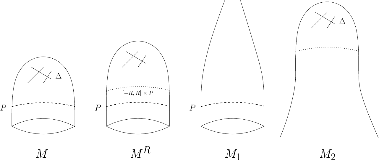
Refer to caption — Figure 1. Splitting $M$ along $P$ .

For the rest of this section we will restrict our attention only to $W=M\setminus\Sigma$ . We denote by $J_{W}$ the restriction of the almost complex structure $J_{M}$ to $W$ . Put

W^{-}=M^{-},\quad W^{+}=M^{+}\setminus\Sigma,\quad W^{R}=M^{R}\setminus\Sigma.

We endow these manifolds with the restrictions of the almost complex structures we have just defined on $M^{-}$ , $M^{+}$ , $M^{R}$ , i.e. $J_{W}$ and $J_{R}$ . The reason for defining all these structures beforehand on $M$ is that later on in §13 we will use these structures to obtain an analogous Floer-Gysin sequence for $\Gamma_{L}$ viewed as a Lagrangian submanifold of $M$ .

The construction above implies that replacing the almost complex structure $J$ on $M$ (resp. $W$ ) by $J_{R}$ (with a large $R$ ) is holomorphically equivalent to stretching the manifold $M$ (resp. $W$ ) along $P$ in the sense of SFT [BEH+, EGH]. We denote by

\mathcal{J}=\mathcal{J}(J_{\Sigma},U,R_{0})=\left\{J_{R}\,\left|\,R>R_{0}\right.\right\}

the space of the stretched complex structures.

For $J\in\mathcal{J}$ denote by

\mathcal{P}_{0}(J)=\bigcup_{\delta(x,y,\mathbf{A})=0}\mathcal{P}(x,y,\mathbf{A};\widetilde{\mathscr{D}}_{\varepsilon})

the union of moduli spaces of pearl trajectories with zero virtual dimension (for any critical points $x,y$ ) for $\Gamma_{L}\subset W$ .

Given $r>0$ , denote by

E_{r}^{*}=E_{r}\setminus\Sigma\subset\mathcal{N}

the punctured disk bundle or radius $r$ over $\Sigma$ . For $0<r_{1}<r_{2}$ denote by

E_{r_{1},r_{2}}=E_{r_{2}}\setminus\textnormal{Int\,}E_{r_{1}}

the (closed) annulus bundle over $\Sigma$ of inner radius $r_{1}$ and outer radius $r_{2}$ . We call it the $(r_{1},r_{2})$ -annulus bundle of $\mathcal{N}$ over $\Sigma$ .

The purpose of working with almost complex structures in $\mathcal{J}$ is the following:

Proposition 5.0.1.

There exists $R_{0}>0$ such that for every $J_{R}$ as described above with $R>R_{0}$ the following holds: every pearly trajectory $\gamma\in\mathcal{P}_{0}(J_{R})$ is contained in the image $F(E_{r_{0},r_{0}+\varepsilon})$ of the $(r_{0},r_{0}+\varepsilon)$ -annulus bundle of $\mathcal{N}$ under $F$ .

Before proving this proposition we derive an important corollary. From now on we will fix the constant $R_{0}$ which is large enough (so that the conclusions of Proposition 5.0.1 hold) and will work with $J_{R}$ where $R>R_{0}$ . We call $\mathcal{J}=\mathcal{J}(J_{\Sigma},U,R_{0})$ the space of admissible almost complex structures. The following corollary is an immediate consequence of Proposition 5.0.1.

Corollary 5.0.2.

Let $\mathscr{D}=(f,(\cdot,\cdot),J_{\Sigma})$ be auxiliary data with generic $J_{\Sigma}$ , and $\widetilde{\mathscr{D}}_{\varepsilon}=(f_{\varepsilon},X_{\varepsilon},J)$ as in §4 where the almost complex structure $J$ is admissible. Then any $\gamma\in\mathcal{P}_{0}(J)$ projects via $\pi$ to a genuine pearly trajectory on $\Sigma$ .

Note that the index of the projection $\pi(\gamma)$ might sometimes be $1$ rather than $0$ .

Remark 5.0.3.

As we will see in the proof of Proposition 5.0.1 below, the conclusions of Proposition 5.0.1 and Corollary 5.0.2 continue to hold also for pearly trajectories $\gamma\in\mathcal{P}(x,y,\mathbf{A};\widetilde{\mathscr{D}}_{\varepsilon})$ with $\delta(x,y,\mathbf{A})=1$ provided that the minimal Chern number $C_{\Sigma}$ of $\Sigma$ is at least $2$ . Here by the minimal Chern number of $\Sigma$ we mean the following number: $C_{\Sigma}=\min\{c_{1}^{\Sigma}(S)\mid S\in\pi_{2}(\Sigma),\,c_{1}^{\Sigma}(S)>0\}$ .

Proof of Proposition 5.0.1.

First of all note that by the maximum principle every non-constant $J$ -holomorphic disk (for $J\in\mathcal{J}$ ) $u:(D,\partial D)\to(W,\Gamma_{L})$ must satisfy $u(\textnormal{Int\,}D)\subset W\setminus E_{r_{0}}$ . The main part of the proof is to show that for $R_{0}\gg 0$ the following holds: for every $R\geq R_{0}$ all $J_{R}$ -holomorphic disks $u$ that participate in index $0$ pearly trajectories (for $(W,\Gamma_{L})$ ) have their images lying inside $E_{r_{0}+\varepsilon}$ .

Below we will refer to the results of [BEH+]. We remark that the statements of that paper hold also for holomorphic curves with boundary on Lagrangian submanifolds.

Put $W^{+}_{\infty}=(-\infty,0]\times P\cup_{\partial}W^{+}$ and $W^{-}_{\infty}=W^{-}\cup_{\partial}[0,\infty)\times P$ each glued along the boundary. The almost complex structure $J_{W}$ on $W^{+}$ and $W^{-}$ is extended to the cylindrical ends by invariance under transtaltion in $t$ coordinate. (One smoothens the resulting almost complex structures near the boundary in the fiber direction in a standard way). Set $(W^{\infty},J^{\infty})$ to be equal to the disjoint union $W^{+}_{\infty}\cup W^{-}_{\infty}$ , each endowed with the preceding almost complex structures. This way, the split manifold $(W^{\infty},J^{\infty})$ can be considered as a limit of $(W^{R},J_{R})$ when $R\to\infty$ , in the sense of [BEH+, EGH]. See figure 1.

Assume by contradiction, that for a generic almost complex structure $J_{\Sigma}$ on $\Sigma$ the statement of the proposition is not true, that is, for any $R>0$ there exists a pearly trajectory $\gamma\in\mathcal{P}_{0}(J_{R})$ which leaves the image of the $(r_{0}+\varepsilon)$ -disk bundle. Let $R_{n}$ be a sequence of stretching parameters with $R_{n}\longrightarrow\infty$ and let $\gamma_{n}\in\mathcal{P}_{0}(J_{R_{n}})$ be a sequence of pearly trajectories with zero index which leave the $(r_{0}+\varepsilon)$ -disk bundle. Under the holomorphic identification between $(W,J_{R})$ and $(W^{R},J_{R})$ , we have a sequence of manifolds $W^{R_{n}}$ together with a sequence of pearly trajectories in $W^{R_{n}}$ . We will use the same notation $\gamma_{n}$ for these trajectories.

For simplicity of notation, we assume that each $\gamma_{n}$ contains a single holomorphic disk $u_{n}:(D,\partial D)\to(W^{R_{n}},\Gamma_{L})$ . (The general case is similar.) Restricting ourselves to a subsequence if needed, we may assume that all $u_{n}$ have the same Maslov index. We denote by $u^{\prime}_{n}:(D,\partial D)\to(W,\Gamma_{L})$ the disks corresponding to $u_{n}$ via $\lambda_{R}$ , i.e. $u^{\prime}_{n}=\lambda_{r}\circ u_{n}$ .

Using the notation of [BEH+], the $\omega$ -energy of a $J$ -holomorphic curve $u$ in $W^{R}$ translates in our notation to the following:

E_{\omega}(u)=\int_{u^{-1}(W^{+}\cup W^{-})}u^{*}\omega+\int_{u^{-1}([-R,R]\times P)}u^{*}\pi_{\Sigma}^{*}\omega_{\Sigma}.

In view of monotonicity of $\Gamma_{L}$ , the area of the disks ${u^{\prime}}_{n}:D\to W$ satisfies $\int_{D}{u^{\prime}}_{n}^{*}\omega=C$ , where the constant $C$ is independent of $n$ . A simple computation (based on (2)) shows that:

\int_{u^{-1}([-R,R]\times P)}{u}^{*}\pi_{\Sigma}^{*}\omega_{\Sigma}\leq\int_{u^{-1}([-R,R]\times P)}{u}^{*}\lambda_{R}^{*}\omega.

It follows that $E_{\omega}(u_{n})\leq C$ for every $n$ . Lemma 9.2 of [BEH+] implies then a uniform bound on the full energy $E(u_{n})$ (see [BEH+] for the definition of this energy).

Theorem 10.3 of [BEH+] describes the compactification of the space of $J$ -holomorphic curves $\{u:D\to(W^{R},J_{R})\,|\,E(u)\leq C\}$ . According to this result, there is a subsequence $u_{n_{k}}$ of $u_{n}$ which converges to a so-called holomorphic building $\overline{u}$ in $W^{\infty}$ . This $\overline{u}$ is a disconnected $J_{\infty}$ -holomorphic curve which consists of the following connected components:

•

a $J$ -holomorphic map $u_{1}:(S_{1},\partial S_{1})\to(W^{+}_{\infty},\Gamma_{L})$ , where $S_{1}$ is a disk with one or more punctures. Near these punctures $u_{1}$ is asymptotically cylindrical and converges to a periodic orbit of the Reeb vector field of $(P,\alpha)$ . (Here $\alpha$ is the connection $1$ -form as chosen in §2.2.) Note that due to our choice of $\alpha$ the periodic orbits of the Reeb vector field are precisely the fibres of the circle bundle $P\to\Sigma$ .
•

a number of $J$ -holomorphic maps, each of them looks like $u_{2}:S_{2}\to W^{-}_{\infty}$ where $S_{2}$ is a sphere with one or more punctures. $u_{2}$ is asymptotically cylindrical near each puncture in a similar way to $u_{1}$ . For simplicity we will assume that there exists one such map. In the case there are many, the argument is the same.
•

in addition, $\overline{u}$ may contain a number of $J$ -holomorphic maps $u_{i}:S_{i}\to\mathbb{R}\times P$ where each $S_{i}$ is a sphere with one or more punctures each. $u_{i}$ are asymptotically cylindrical near each puncture as well.

Moreover, the components of $\overline{u}$ fit over the punctures, so they admit gluing to a topological disk.

Coming back to our situation, there is a subsequence of $\{\gamma_{n}\}$ that converges to a pearly-like trajectory $\overline{\gamma}$ which has instead of a usual holomorphic disk a $J_{\infty}$ -holomorphic building $\overline{u}$ attached. We claim that this implies that the virtual dimension of the corresponding moduli space of trajectories is positive. This will give a contradiction to our initial assumption that $\gamma_{n}\in\mathcal{P}_{0}(J_{R_{n}})$ . Note that apriori, in addition to the above limit, one may have all possible limits of pearly trajectories as described in [BC4, BC6], e.g. breaking of gradient trajectories, bubbling of disks or spheres etc. For simplicity of notation, we assume that the holomorphic building $\overline{u}$ consists only of two components: a punctured disk $u_{1}:(S_{1},\partial S_{1})\to W^{+}_{\infty}$ and a punctured sphere (i.e. a finite energy plane) $u_{2}:S_{2}\to W^{-}_{\infty}$ , where each component has a single puncture. The general case can be treated in a similar way to what is done below.

By the definition of $J_{\infty}$ on $W^{+}_{\infty}$ , the projection $\pi_{1}:W^{+}_{\infty}\to\Sigma$ is $(J_{\infty},J_{\Sigma})$ -holomorphic, hence $\pi_{1}$ sends $u_{1}$ to a punctured disk $\pi_{1}\circ u_{1}:(S_{1},\partial S_{1})\to(\Sigma,L)$ . The periodic orbits at infinity project via $\pi_{1}$ to single points in $\Sigma$ since they are exacly the fibres of the circle bundle $P\to\Sigma$ . Due to the asymptotic behavior of $u_{1}$ near the puncture $z$ we obtain that $\pi_{1}\circ u_{1}$ extends continuously at the puncture. Therefore $z$ is a removable singularity and $\pi_{1}\circ u_{1}$ becomes a genuine $J_{\Sigma}$ -holomorphic disk.

We would like now to project $u_{2}:S_{2}\to W^{-}_{\infty}$ to $\Sigma$ . However, this cannot be done directly. Recall that on $W^{-}_{\infty}$ we have a projection defined only away from the skeleton, $\pi_{2}:W^{-}_{\infty}\setminus\Delta\to\Sigma$ , and moreover this projection is not holomorphic on $U\setminus\Delta$ . We deal with this difficulty as follows. As $\text{codim }\Delta>2$ , we can always perturb $u_{2}$ near $\Delta$ (in a non-holomorphic way) and obtain a new surface ${\widetilde{u}_{2}}:S_{2}\to W^{-}_{\infty}$ with ${\widetilde{u}_{2}}(S_{2})\cap\Delta=\emptyset$ . Then $\pi_{2}\circ{\widetilde{u}_{2}}$ gives a (not necessarily holomorphic) sphere $v:S^{2}\to\Sigma$ . (Again, the puncture goes to a point at which we have a removable singularity.) We claim that $v$ has a positive Chern number. To see this recall that $\Sigma$ is monotone, hence $c_{1}^{\Sigma}=\lambda[\omega_{\Sigma}]$ on $\pi_{2}(\Sigma)$ for some $\lambda>0$ . Therefore we have:

(11)

c_{1}^{\Sigma}([v])=\lambda\omega_{\Sigma}([v])=\lambda\int_{S_{2}}{\widetilde{u}_{2}}^{*}\pi_{2}^{*}\omega_{\Sigma}=\lambda\int_{{\widetilde{u}_{2}}^{-1}(W^{-})}{\widetilde{u}_{2}}^{*}\pi_{2}^{*}\omega_{\Sigma}+\lambda\int_{{\widetilde{u}_{2}}^{-1}(W^{-}_{\infty}\setminus W^{-})}{\widetilde{u}_{2}}^{*}\pi_{2}^{*}\omega_{\Sigma}.

The 2’nd term is non-negative since $\pi_{2}$ is holomorphic on $W^{-}_{\infty}\setminus W^{-}$ . As for the first term we have:

\int_{{\widetilde{u}_{2}}^{-1}(W^{-})}{\widetilde{u}_{2}}^{*}\pi_{2}^{*}\omega_{\Sigma}=e^{(r_{0}+\varepsilon)^{2}}\int_{{\widetilde{u}_{2}}^{-1}(W^{-})}{\widetilde{u}_{2}}^{*}\omega=e^{(r_{0}+\varepsilon)^{2}}\int_{u_{2}^{-1}(W^{-})}u_{2}^{*}\omega>0,

where the equalities follow from Stokes theorem (recall that the perturbation ${\widetilde{u}_{2}}$ took place away from the boundary $u_{2}(\partial S_{2})$ ). The last inequality holds because $u_{2}$ is holomorphic. This proves that $c_{1}^{\Sigma}([v])>0$ .

Next, replace in the “pearly” trajectories $\overline{\gamma}$ the holomorphic curve $u_{2}$ by its perturbation $\widetilde{u}_{2}$ . We continue to denote this trajectory by $\overline{\gamma}$ . Consider now its projection $\pi\circ\overline{\gamma}$ to $\Sigma$ . The projected trajectory is a pearly trajectory on $\Sigma$ whose disk $\pi_{1}\circ u_{1}$ has a non-holomorphic sphere $v$ attached, and moreover $c_{1}^{\Sigma}([v])>0$ . ( $v$ cannot be constant because in this case $u_{2}$ would have zero $\omega$ -energy.) Denote by $\gamma_{\Sigma}$ the trajectory obtained from $\pi\circ\overline{\gamma}$ after removing the sphere $v$ . Note that $\gamma_{\Sigma}$ is a genuine pearly trajectory.

Denote by $A\in H_{2}(W\setminus\Delta,\Gamma_{L})$ the total homology class in $\overline{\gamma}$ and by $B\in H_{2}(\Sigma,L)$ the total homology class in $\gamma_{\Sigma}$ after the sphere $[v]$ is removed, i.e. $B=\pi_{*}(A)-[v]$ . Let $\widetilde{x},\widetilde{y}$ be the starting and the ending critical points for $\overline{\gamma}$ . Thus $\gamma_{\Sigma}$ connects $x_{\Sigma}=\pi(\widetilde{x})$ with $y_{\Sigma}=\pi(\widetilde{y})$ . As $\gamma_{\Sigma}$ is a genuine pearly trajectory and $J_{\Sigma}$ is regular, the virtual dimension of the corresponding moduli space $\mathcal{P}(x_{\Sigma},y_{\Sigma},B;J_{\Sigma})$ is non-negative:

|x_{\Sigma}|-|y_{\Sigma}|+\mu_{L}(B)-1\geq 0

Note that $|\widetilde{y}|\geq|y_{\Sigma}|$ and $|\widetilde{x}|\leq|x_{\Sigma}|+1$ . Therefore

|y_{\Sigma}|-|x_{\Sigma}|\leq|\widetilde{y}|-|\widetilde{x}|+1.

We also have:

(12)

\mu_{\Gamma_{L}}([\overline{u}])=\mu_{\Gamma_{L}}(A)=\mu_{L}(\pi_{*}A)=\mu_{L}(B)+2c_{1}^{\Sigma}([v])\geq\mu_{L}(B)+2.

All together this gives us

|\widetilde{y}|-|\widetilde{x}|+\mu_{\Gamma_{L}}([\overline{u}])-1\geq|y_{\Sigma}|-|x_{\Sigma}|-1+\mu_{L}(B)+2-1=\left(|y_{\Sigma}|-|x_{\Sigma}|+\mu_{L}(B)-1\right)+1>0,

which contradicts the assumption that we are in a moduli space of index $0$ .

The other configurations that might appear in the limit of $\gamma_{n}$ can be dealt with by a combination of the argument above and the compactification of spaces of pearly trajectories as described in [BC4, BC6]. ∎

Remark 5.0.4.

Note that in the proof of Proposition 5.0.1 we have used only transversality for spaces of pearly trajectories on $(\Sigma,L)$ , not for $(W,\Gamma_{L})$ .

6. Transversality

The aim of this section is to establish the needed transversality results for the spaces of pearly trajectories involved in the quantum cohomologies of $L$ and $\Gamma_{L}$ that appear in our long exact sequence. While the general theory of pearl homology [BC4, BC6] assures this transversality for generic choice of auxiliary data, this is apriori not the case in our setting. For example, the almost complex structures $J$ that we use on $W$ are not arbitrary as they depend strongly on $J_{\Sigma}$ , in particular they cannot be assumed to be generic in the strict sense of the word. Still we will see below that transversality can be still achieved by taking $J_{\Sigma}$ to be generic.

6.1. Regularity of $J_{R}$

Holomorphic disks in $u:(D,\partial D)\to(W,\Gamma_{L})$ fall into two types. Those who go out from $E_{r_{0}+\varepsilon}$ and those who remain entirely inside $E_{r_{0}+\varepsilon}$ . Transversality for the first type is easy to achieve: recall that in our set of admissible $J$ ’s there was no restriction on $J$ outside of $E_{r_{0}+\varepsilon}$ . Thus we can take $J$ to be generic on $M\setminus E_{r_{0}+\varepsilon}$ , and the general theory [MS] assures that such $J$ ’s will be regular for this type of disks.

We now turn to those disks that are entirely contained in $E_{r_{0}+\varepsilon}$ . In fact, as we saw in §5, these are the most relevant disks, as all pearly trajectories of index $0$ involve only disks inside $E_{r_{0}+\varepsilon}$ .

We want to show that for a choice of a regular $J_{\Sigma}$ on $\Sigma$ any admissible $J_{R}$ (as it is constructed in §5) satisfies regularity conditions on the disk bundle $E_{r_{0}+\varepsilon}$ . This would imply that the moduli space $\mathcal{M}^{*}(A;J_{R})$ of simple $J_{R}$ -holomorphic disks $u:(D,\partial D)\to(E_{r_{0}+\varepsilon},\Gamma_{L})$ with $u_{*}([D])=A$ is a smooth finite dimensional manifold.

To prove the statement, we replace $(E_{r_{0}+\varepsilon},J_{R})$ by a disk bundle $E_{A(R)}\subset(\mathcal{N},J_{\mathcal{N}})$ using the identifications defined in §5, where $A(R)$ depends on $R$ . Below we will use the same notation $\Gamma_{L}$ for the image of $\Gamma_{L}$ in $E_{R}$ . Recall from [MS] (see §3.1 there) that regularity of an almost complex structure means the surjectivity of the linearization of the $\bar{\partial}$ –operator $D_{u}$ at each $J$ -holomorphic disk $u:(D,\partial D)\to(E_{R},\Gamma_{L})$ .

Let $u:(D,\partial D)\to(E_{R},\Gamma_{L})$ be a holomorphic disk. Note, that the projection $\pi\circ u:(D,\partial D)\to(\Sigma,L)$ is $J_{\Sigma}$ -holomorphic. Pick a holomorphic trivialization $g:(\pi\circ u)^{*}\mathcal{N}\to D\times\mathbb{C}$ . Using this trivialization, we associate to $u$ a pair of holomorphic maps $(u_{\Sigma},u_{\mathcal{N}})$ where $u_{\Sigma}=\pi\circ u$ and $u_{\mathcal{N}}:D\to\mathbb{C}$ is the projection of $g\circ u$ to the second component. Accordingly, we have an associated pair of linearizations of the $\bar{\partial}$ –operator $(D_{u_{\Sigma}},D_{u_{\mathcal{N}}})$ . For the surjectivity of $D_{u}$ it is sufficient to show that both $D_{u_{\Sigma}}$ and $D_{u_{\mathcal{N}}}$ are surjective. This property holds for $D_{u_{\Sigma}}$ from the regularity of $J_{\Sigma}$ . The same is true for $D_{u_{\mathcal{N}}}$ since the almost complex structure in the fiber $\mathbb{C}$ (multiplication by $i$ ) is regular.

6.2. Transversality for pearly trajectories of index $0$

Let $\mathscr{D}=(f,(\cdot,\cdot),J_{\Sigma})$ be a choice of Morse function, metric on $L$ and almost complex structure on $\Sigma$ . Recall from §4.1 that in order to construct $\widetilde{\mathscr{D}}_{\varepsilon}$ we need the following additional auxiliary objects: $(\nabla,\alpha,h,J_{R})$ , where $\nabla$ is a connection as chosen in §2.2, $\alpha$ represents a choice of cutoff functions near $\textnormal{Crit}(f)$ and $h$ stands for a collection of Morse functions $S^{1}\to\mathbb{R}$ , as was described in §4.1. Here $J_{R}$ is an admissible almost complex structure on $M$ which is induced from $J_{\Sigma}$ and satisfies Proposition 5.0.1. We will use the same notation $J_{R}$ for the induced almost complex structure on $E_{r_{0}+\varepsilon}$ .

Denote by $Q_{f}$ the image of the embedding:

(L\setminus\textnormal{Crit}(f))\times\mathbb{R}_{>0}\lhook\joinrel\longrightarrow L\times L,\quad(x,t)\longmapsto(x,\Phi^{f}_{t}(x)),

where $\Phi^{f}_{t}$ is the negative gradient flow of $f$ . Similarly, define $Q_{\widetilde{X}_{\varepsilon}}\subset\Gamma_{L}\times\Gamma_{L}$ to be the image of the embedding:

(\Gamma_{L}\setminus\textnormal{Crit}(f_{\epsilon}))\times\mathbb{R}_{>0}\lhook\joinrel\longrightarrow\Gamma_{L}\times\Gamma_{L},\quad(x,t)\longmapsto(x,\Phi^{X}_{t}(x))

where $\Phi^{X}_{t}$ is the flow of $\widetilde{X}_{\varepsilon}$ . Let $\mathcal{M}(A,J)$ be the moduli space of holomorphic disks in the homology class $A\in H_{2}(W,\Gamma_{L})$ . For a sequence $\mathbb{A}=(A_{1},\ldots,A_{l})$ of non-zero classes $A_{i}\in H_{2}(W,\Gamma_{L})$ put

\mathcal{M}(\mathbb{A},J)=\mathcal{M}(A_{1},J)\times\ldots\times\mathcal{M}(A_{l},J).

The space $\mathcal{M}(\mathbf{A},J)$ comes with an evaluation map:

ev_{\mathbb{A}}:\mathcal{M}(\mathbb{A},J)\longrightarrow\Gamma_{L}^{\times 2l},\quad ev_{\mathbb{A}}(u_{1},\ldots,u_{l})=\left(u_{1}(-1),u_{1}(1),\ldots,u_{l}(-1),u_{l}(1)\right).

Similarly we have the spaces $\mathcal{M}^{*}(A_{i},J)\subset\mathcal{M}(A_{i},J)$ of simple disks and $\mathcal{M}^{*}(\mathbb{A},J)=\mathcal{M}^{*}(A_{1},J)\times\ldots\times\mathcal{M}^{*}(A_{l},J)\subset\mathcal{M}(\mathbf{A},J)$ . Note that in general $\mathcal{M}(\mathbf{A},J)$ might not be a smooth manifold (even for generic $J$ ’s). On the other hand, by what we have just seen in §6.1 for generic admissible $J$ the spaces $\mathcal{M}^{*}(\mathbf{A},J)$ are smooth manifolds. (See [BC4] for more details on this issue.) Denote by $H\subset\textnormal{Aut}(D)\cong PSL(2,\mathbb{R})$ the subgroup of all biholomophisms $\sigma:D\to D$ which fix the two points $-1,1\in D$ , $\sigma(\pm 1)=\pm 1$ . The group $H$ acts on $\mathcal{M}^{*}(A_{i},J)$ by parametrization, i.e. $\sigma\cdot u=u\circ\sigma^{-1}$ . Applying this to each factor of $\mathcal{M}^{*}(A_{i},J)$ we obtain an action of $H^{\times l}$ on $\mathcal{M}^{*}(\mathbf{A},J)$ .

Let $\tilde{x},\,\tilde{y}\in{\rm{Crit\/}}\;(\widetilde{X}_{\varepsilon})$ . Put

\widetilde{R}=W^{s}_{\tilde{x}}\times(Q_{\widetilde{X}_{\varepsilon}})^{\times(l-1)}\times W^{u}_{\tilde{y}}.

With this notation we have:

\mathcal{P}(\tilde{x},\tilde{y},\mathbf{A};\widetilde{\mathscr{D}}_{\varepsilon})=ev_{\mathbf{A}}^{-1}(\widetilde{R})/H^{\times l}.

Proposition 6.2.1.

Let $\mathscr{D}=(f,(\cdot,\cdot),J_{\Sigma})$ be generic data on $(\Sigma,L)$ . Let $J_{R}$ be an admissible almost complex structure as in Proposition 5.0.1, and let $h$ be a generic collection of functions. Let $\tilde{x},\,\tilde{y}\in{\rm{Crit\/}}\;(\widetilde{X}_{\varepsilon})$ , $\mathbf{A}$ with $\delta=\delta(\tilde{x},\tilde{y},\mathbf{A})\leq 0$ . Then:

(1)

Every tuple of holomorphic disks $\mathbf{u}\in\mathcal{M}(\mathbb{A},J_{R})$ that participates in $\mathcal{P}(\tilde{x},\tilde{y},\mathbf{A};\widetilde{\mathscr{D}}_{\varepsilon})$ consists of simple and absolutely distinct disks (see Definition 3.1.1 in [BC4] for the definition).
(2)

The restriction of $ev_{\mathbf{A}}$ to $\mathcal{M}^{*}(\mathbf{A},J_{R})$ is transverse to $\widetilde{R}$ .

In particular the spaces of pearly trajectories $\mathcal{P}(\tilde{x},\tilde{y},\mathbf{A};\widetilde{\mathscr{D}}_{\varepsilon})$ are smooth manifolds of dimension $\delta$ . (In particular when $\delta<0$ they are void.) Moreover, when $\delta=0$ these manifolds are compact, hence consist of a finite number of elements.

Recall that by the results of [BC4], for a generic choice of data $\mathscr{D}$ , the same result as in Proposition 6.2.1 holds for $(\Sigma,L)$ whenever the virtual dimension $\delta(x,y,\pi_{*}(A))$ is $\leq 1$ . The main point in Proposition 6.2.1 is that this continues to hold for also for $(W,\Gamma_{L})$ even if one uses the (apriori non-generic) data $\widetilde{\mathscr{D}}_{\varepsilon}$ which depends on $\mathscr{D}$ . We remark however that in contrast to $(\Sigma,L)$ , for $(W,\Gamma_{L})$ we have to restrict only to pearly trajectories of index $0$ . The reason is that the proof goes by comparing the transversality of $ev_{\mathbf{A}}$ (for $(W,\Gamma_{L})$ with that of $ev_{\pi_{*}(\mathbf{A})}$ (for $(\Sigma,L)$ ). If $\gamma$ is a pearly trajectory on $(W,\Gamma_{L})$ of index $\delta(\gamma)$ then the index $\delta(\pi(\gamma))$ of its projection satisfies: $\delta(\pi(\gamma))\leq\delta(\gamma)+1$ , where equality might occur. Thus if $\delta(\gamma)=1$ we might have $\delta(\pi(\gamma))=2$ and transversality for index $2$ trajectory is not known. Therefore, we restrict on $(W,\Gamma_{L})$ to spaces of virtual dimension $0$ only. However, as we will see in §6.3 this is enough for our purposes.

Proof of Proposition 6.2.1.

In view of Proposition 5.0.1 we may assume that all disks involved in pearly trajectories corresponding to $\textnormal{Image\,}(ev_{\mathbf{A}})\cap\widetilde{R}$ lie inside $E_{r_{0}+\varepsilon}$ . Therefore we can project all pearly trajectories from $\mathcal{P}(\tilde{x},\tilde{y},\mathbf{A};\widetilde{\mathscr{D}}_{\varepsilon})$ and obtain pearly trajectories on $(\Sigma,L)$ . We will also view each of the classes $A_{i}$ in $\mathbf{A}$ as elements of $H_{2}(E_{r_{0}+\varepsilon},\Gamma_{L})$ . An important point that will be used a few times in the proof below is that if $\gamma\in\mathcal{P}(\Gamma_{L};\tilde{x},\tilde{y},A;\widetilde{D}_{\varepsilon})$ has index $0$ then its projection $\pi(\gamma)$ to $\Sigma$ has index $\leq 1$ . Therefore, if $\mathscr{D}$ is generic then $\pi(\gamma)$ consists only of simple and absolutely distinct disks and moreover we have transversality for $ev_{\pi_{*}(\mathbf{A})}$ .

Denote by $ev^{*}_{\mathbf{A}}$ the restriction of $ev_{\mathbf{A}}$ to $\mathcal{M}^{*}(\mathbf{A},J_{R})$ . Write

\mathcal{M}^{*,d}(\mathbf{A},J_{R})\subset\mathcal{M}^{*}(\mathbf{A},J_{R})

for the open subset of those tuples $\mathbf{u}=(u_{1},\ldots,u_{l})$ which consist of absolutely distinct disks in the sense of [BC4] (see Definition 3.1.1 there). (Absolutely distinct means roughly speaking that no disk $u_{i}$ has its image entirely covered by the union of the rest of the disks, i.e. that $u_{i}(D)\not\subset\cup_{j\neq i}u_{j}(D)$ for every $i$ .) Denote by $ev^{*,d}_{\mathbf{A}}$ the restriction of $ev_{\mathbf{A}}$ to the latter subspace. Note that by the discussion in §6.1 both $\mathcal{M}^{*}(\mathbf{A},J_{R})$ and $\mathcal{M}^{*,d}(\mathbf{A},J_{R})$ are smooth manifolds for a generic admissible $J_{R}$ .

The first step of the proof is to show that $ev^{*,d}_{\mathbf{A}}$ is transverse to $\widetilde{R}$ .

Let $\mathbb{q}=(q_{1},\ldots,q_{2l})\in\Gamma_{L}^{\times 2l}$ belong to the intersection of $\text{Image}(ev^{*,d}_{\mathbb{A}})$ and $\widetilde{R}$ . Pick a sequence of disks $\mathbb{\tilde{u}}=(\tilde{u}_{1},\ldots,\tilde{u}_{l})\in\mathcal{M}^{*,d}(\mathbb{A},J_{R})$ such that $ev^{*,d}_{\mathbb{A}}(\mathbb{\tilde{u}})=\mathbf{q}$ . We denote the projections $\pi(\mathbb{\tilde{u}}),\pi(\tilde{x}),\pi(\tilde{y})$ to $\Sigma$ by $\mathbb{u}=(u_{1},\ldots,u_{l}),x$ and $y$ , respectively.

The proof goes by comparison of $ev^{*,d}_{\mathbf{A}}$ and $\widetilde{R}$ with their counterparts in $(\Sigma,L)$ namely $ev^{*,d}_{\pi_{*}A}$ and $R=W^{s}_{x}\times(Q_{-\nabla f})^{\times(l-1)}\times W^{u}_{y}$ , which are assumed to be transverse (due to a generic choice of $\mathscr{D}$ ). Note that our choice of auxiliary data implies that $R=\pi(\widetilde{R})$ . Similarly, the lifting Lemma 7.1.1 (see §7 below) together with the projection property of $J_{R}$ ensure that $ev^{*,d}_{\pi_{*}A}=\pi(ev^{*,d}_{A})$ .

At each $q_{i}$ we choose a splitting $T_{q_{i}}\Gamma_{L}\simeq H^{\nabla}_{q_{i}}\oplus\mathbb{R}$ where $H^{\nabla}$ denotes the horizontal distribution of the connection $\nabla$ and $\mathbb{R}$ is the tangent space of the fiber. Then $T_{\mathbf{q}}\Gamma_{L}^{\times 2l}\simeq\bigoplus H^{\nabla}_{q_{i}}\oplus\mathbb{R}^{\times 2l}$ and the restriction $D\pi:\bigoplus H^{\nabla}_{q_{i}}\times\{0\}\to T_{\pi(\mathbf{q})}L^{\times 2l}$ is an isomorphism. Using the splitting $T_{\mathbf{q}}\Gamma_{L}^{\times 2l}\simeq\bigoplus H^{\nabla}_{q_{i}}\oplus\mathbb{R}^{\times 2l}$ we introduce coordinates $(v,r_{1},\ldots,r_{2l})$ on $T_{\mathbf{q}}\Gamma_{L}^{\times 2l}$ where $v\in\bigoplus H^{\nabla}_{q_{i}}$ and $r_{k}\in\mathbb{R}$ .

By Lemma 7.1.1 $J_{\Sigma}$ -holomorphic disks $u:(D^{2},\partial D^{2})\to(\Sigma,L)$ correspond to one-parametric families of disks $\tilde{u}:(D^{2},\partial D^{2})\to(E_{r_{0}+\varepsilon},\Gamma_{L})$ which are parametrized by $S^{1}$ . More exactly, if $\tilde{u}$ is one such lift, then the others are given by rotations $\{e^{i\theta}\cdot\tilde{u}\}$ in the fibers of $E_{r_{0}+\varepsilon}$ . Therefore, $\mathcal{M}^{*}(\mathbb{A},J_{R})$ admits an $(S^{1})^{\times l}$ action $G$ which corresponds to independent rotation of the lifts of each disk $u_{k}$ . This implies that $ev^{*,d}_{\mathbb{A}}(G\,\mathbb{\tilde{u}})\subseteq\text{Image}(ev^{*,d}_{\mathbb{A}})$ . Consequently, $V_{1}=T_{\mathbf{q}}ev^{*,d}_{\mathbb{A}}(G\,\mathbb{\tilde{u}})\subseteq T_{\mathbf{q}}\text{Image}(ev^{*,d}_{\mathbb{A}})$ . Note, that $V_{1}=\{0\}\times\{(r_{1},r_{1},r_{2},r_{2},\ldots,r_{l},r_{l})\}_{r_{i}\in\mathbb{R}}$ in the coordinates described above. On the other hand , each $Q_{\widetilde{X}_{\varepsilon}}$ also admits a similar $S^{1}$ -action. This gives rise to an $(S^{1})^{\times(l-1)}$ -action on $\widetilde{R}$ which implies that $V_{2}=\{0\}\times\{(0,r_{1},k_{1}r_{1},\ldots,r_{l-1},k_{l-1}r_{l-1},0)\}_{r_{i}\in\mathbb{R}}\subseteq T_{\mathbf{q}}\widetilde{R}$ (The constants $k_{i}$ are equal to $1$ in the case when the corresponding gradient trajectory segment does not pass through any neighbourhood $\mathcal{U}$ of a critical point. In the case when it does, we still have $k_{i}\neq 0$ .)

Now we analyze the possible configurations of the critical points $\tilde{x},\,\tilde{y}$ . Below we will use the following observation: let $\pi:U_{1}\to U_{2}$ be a surjective linear map. Let $V$ be a linear subspace of $U_{1}$ . Assume that $\ker(\pi)\subseteq V$ . Then $V=U_{1}$ if and only if $\pi(V)=U_{2}$ .

•

$\tilde{x}=x^{\prime}$ . In this case $T_{q_{1}}W^{s}_{\tilde{x}}$ contains the subspace $\{0\}\times\mathbb{R}$ , therefore $V_{3}=\{0\}\times\{(r,0,\ldots,0)\}_{r\in\mathbb{R}}\subseteq T_{\mathbf{q}}\widetilde{R}$ . We now have: $V_{1}+V_{2}+V_{3}=\{0\}\times\mathbb{R}^{\times 2l}\subseteq T_{\mathbf{q}}\text{Image}(ev^{*,d}_{\mathbb{A}})+T_{\mathbf{q}}\widetilde{R}$ . That is, the right-hand sum contains the complementary subspace $\{0\}\times\mathbb{R}^{\times 2l}$ which is the kernel of the projection $\pi:T_{\mathbf{q}}\Gamma_{L}^{2l}\to T_{\pi(\mathbf{q})}L^{2l}$ . The observation above implies that in this case the intersection is transverse if and only if the same is true for the respective projections $\text{Image}(ev^{*,d}_{\pi_{*}\mathbb{A}})$ and $R$ . The latter are assumed to be transverse by a generic choice of the data $\mathscr{D}$ on $(\Sigma,L)$ .
•

$\tilde{y}=y^{\prime\prime}$ . In this case $T_{q_{1}}W^{u}_{\tilde{y}}$ contains the subspace $\{0\}\times\mathbb{R}$ , therefore $V_{3}=\{0\}\times\{(0,\ldots,0,r)\}_{r\in\mathbb{R}}\subseteq T_{\mathbf{q}}\widetilde{R}$ . Once again, $V_{1}+V_{2}+V_{3}=\{0\}\times\mathbb{R}^{\times 2l}$ . Using the same argument as before, we conclude that $ev^{*,d}_{\mathbb{A}}$ and $\widetilde{R}$ are transverse whenever their projections on $\Sigma$ are.
•

The only case left to consider is $\tilde{x}=x^{\prime\prime}$ and $\tilde{y}=y^{\prime}$ .

We denote $\widetilde{R}^{\circ}=\{e^{i\theta}\cdot W^{s}_{\tilde{x}}\}_{\theta\in[0,2\pi]}\times(Q_{\widetilde{X}_{\varepsilon}})^{\times(l-1)}\times W^{u}_{\tilde{y}}$ . Using argument similar to that in the previous cases, one can show that $\widetilde{R}^{\circ}$ intersects $\text{Image}(ev^{*,d}_{\mathbb{A}})$ in transverse way. Therefore $K=\widetilde{R}^{\circ}\cap\text{Image}(ev^{*,d}_{\mathbb{A}})$ is a finite-dimensional manifold. It follows from a version of Sard’s theorem, that for almost all values of $\theta_{0}$ , $\widetilde{R}^{\theta_{0}}=\{e^{i\theta_{0}}\cdot W^{s}_{\tilde{x}}\}\times(Q_{\widetilde{X}_{\varepsilon}})^{\times(l-1)}\times W^{u}_{\tilde{y}}$ has transverse intersection with $\text{Image}(ev^{*,d}_{\mathbb{A}})$ . Thus we can avoid non-transversality by a small perturbation of $x^{\prime\prime}$ in its fiber. Such perturbation corresponds to a perturbation of the appropriate Morse function $h_{i}$ as defined in §4. For generic choice of functions $\{h_{i}\}$ this non-transversality phenomenon will not occur.

This concludes the proof that $ev^{*,d}_{\mathbf{A}}$ is transverse to $\widetilde{R}$ .

Next we claim that ${ev_{\mathbf{A}}}^{-1}(\widetilde{R})={ev^{*,d}_{\mathbf{A}}}^{-1}(\widetilde{R})$ , namely that all tuples $\mathbf{u}=(u_{1},\ldots,u_{l})$ that participate in $\mathcal{P}(\tilde{x},\tilde{y},\mathbf{A};\widetilde{\mathscr{D}}_{\varepsilon})$ consist of simple absolutely distinct disks. This can be done either by repeating the arguments from Section 3 of [BC4] or alternatively by looking at the projection $\pi(\gamma)$ of $\gamma$ to $(\Sigma,L)$ . Indeed, if the disks in $\gamma$ are either non-simple or not absolutely distinct then the same would hold for the disks in $\pi(\gamma)$ too. However, this is not the case for $\pi(\gamma)$ since for a generic $\mathscr{D}$ all disks in pearly trajectories of index $\leq 1$ on $(\Sigma,L)$ must be simple and absolutely distinct (see Proposition 3.1.3 in [BC4]).

Finally, the fact that $\mathcal{P}(\tilde{x},\tilde{y},\mathbf{A};\widetilde{\mathscr{D}}_{\varepsilon})$ is compact when $\delta(\tilde{x},\tilde{y},\mathbf{A})=0$ can be proved in a similar way as in Section 3 of [BC4]. One analyzes all possible apriori limits of sequence of pearly trajectories from $\mathcal{P}(\tilde{x},\tilde{y},\mathbf{A};\widetilde{\mathscr{D}}_{\varepsilon})$ and deduces that those configurations that do not appear in $\mathcal{P}(\tilde{x},\tilde{y},\mathbf{A};\widetilde{\mathscr{D}}_{\varepsilon})$ belong to moduli spaces of virtual dimension $<0$ . But such spaces must be void due to the transversality result we have just proved. ∎

6.3. Well-definedness of the pearl complex $\mathcal{C}(\Gamma_{L};\widetilde{\mathscr{D}}_{\varepsilon})$

Having established transversality for the moduli spaces $\mathcal{P}(\Gamma_{L};\tilde{x},\tilde{y},\mathbf{A};\widetilde{\mathscr{D}}_{\varepsilon})$ whenever $\delta(\tilde{x},\tilde{y},\mathbf{A})=0$ we are ready to prove that $\mathcal{C}(\Gamma_{L};\widetilde{\mathscr{D}}_{\varepsilon})$ is well defined and its cohomology is isomorphic to $QH(\Gamma_{L})$ . This is done as follows.

First note that due to Proposition 6.2.1 the pearly differential $\widetilde{d}$ on $\mathcal{C}(\Gamma_{L};\widetilde{\mathscr{D}}_{\varepsilon})$ is well defined as an operator. (Note however that as we have not established transversality for $1$ -dimensional moduli spaces we apriori do not yet that $\widetilde{d}\circ\widetilde{d}=0$ .)

Let $\widetilde{\mathscr{D}}^{\prime}_{\varepsilon}=(f^{\prime}_{\varepsilon},X^{\prime}_{\varepsilon},J^{\prime})$ be a small and generic perturbation of the data $\widetilde{\mathscr{D}}_{\varepsilon}$ where $f^{\prime}_{\varepsilon}=f_{\varepsilon}$ , $(f_{\varepsilon},X^{\prime}_{\varepsilon})$ is negative almost gradient and $J^{\prime}$ is not necessarily admissible (hence can be taken to be really generic). Denote by $\widetilde{d}^{\prime}$ the pearly differential of $\mathcal{C}(\Gamma_{L};\widetilde{\mathscr{D}}^{\prime}_{\varepsilon})$ . By the general theory [BC4, BC6], $\widetilde{d}^{\prime}$ is indeed a differential and

H^{*}(\mathcal{C}(\Gamma_{L};\widetilde{\mathscr{D}}^{\prime}_{\varepsilon}),\widetilde{d}^{\prime})\cong QH^{*}(\Gamma_{L}).

Clearly $\mathcal{C}^{*}(\Gamma_{L};\widetilde{\mathscr{D}}^{\prime}_{\varepsilon})=\mathcal{C}^{*}(\Gamma_{L};\widetilde{\mathscr{D}}_{\varepsilon})$ as graded vector spaces. Finally, the transversality result of Proposition 6.2.1 together with standard arguments imply that $\widetilde{d}=\widetilde{d}^{\prime}$ which proves our claim.

7. Lifting pearly trajectories

Denote by $\mathcal{N}\to\Sigma$ the normal bundle of $\Sigma$ in $M$ , viewed as a complex line bundle as in §2.2. We identify $\Sigma$ with the zero section of $\mathcal{N}$ . We use the connection $\nabla$ on $\mathcal{N}$ to define an almost complex structure $J_{\mathcal{N}}$ on the total space of $\mathcal{N}$ , as was done at the beginning of §5 (see (9) there, where the almost complex structure was denoted by $J_{M}$ ).

In this section we show that any pearly trajectory on $(\Sigma,L)$ (with respect to $\mathscr{D}=(f,(\cdot,\cdot),J_{\Sigma})$ admits a lift to $(\mathcal{N}\setminus\Sigma,\Gamma_{L})$ with respect to the corresponding data $\widetilde{\mathscr{D}}_{\varepsilon}=(f_{\varepsilon},X_{\varepsilon},J_{\mathcal{N}})$ . Due to compactness properties such lifts are contained in a certain disk bundle of $\mathcal{N}$ , hence using the identification $(E_{A(R)},J_{\mathcal{N}})\to(E_{r_{0}+\varepsilon},J_{R})$ induced by $\lambda_{R}$ , one obtains the same result for $(W,\Gamma_{L};J_{R})$ (under assumption that the stretching parameter $R$ is large enough).

Moreover, the set of lifts of any non-constant trajectory is parametrized by $S^{1}$ . Having specified appropriate boundary conditions, one obtains a unique lift, hence in the view of the projection property established in Corollary 5.0.2 in §5 there is one-to-one correspondence between index $0$ pearly trajectories in $(\Sigma,L)$ and those on $(W,\Gamma_{L})$ . More precisely, we will see that for any $x,y\in\text{Crit}(f)$ and $A\in\pi_{2}(\Sigma,L)$ such that $|y|-|x|+\mu(A)-1=0$ , we have:

\#\mathcal{P}(x,y,A;\mathscr{D})=\#\mathcal{P}(x^{\prime},y^{\prime},\pi_{*}^{-1}(A);\widetilde{\mathscr{D}}_{\varepsilon})=\#\mathcal{P}(x^{\prime\prime},y^{\prime\prime},\pi_{*}^{-1}(A);\widetilde{\mathscr{D}}_{\varepsilon}).

Here by $\pi_{*}$ we mean the homomorphism $\pi_{*}:\pi_{2}(W\setminus\Delta,\Gamma_{L})\to\pi_{2}(\Sigma,L)$ which is an isomorphism (see (3) before Proposition 2.4.2), hence it makes sense to write $\pi_{*}^{-1}$ .

7.1. Lifting of disks

Lemma 7.1.1.

Let $u:(D^{2},\partial D^{2})\to(\Sigma,L)$ be a $J_{\Sigma}$ -holomorphic disk. Given $\xi\in\partial D^{2}$ and $\tilde{p}\in\Gamma_{L}\cap\pi^{-1}(u(\xi))$ there is a unique lift $\tilde{u}:(D^{2},\partial D^{2};i)\to(\mathcal{N}\setminus\Sigma,\Gamma_{L};J_{\mathcal{N}})$ of $u$ such that $\tilde{u}(\xi)=\tilde{p}$ .

Proof.

The pull back bundle $(u^{*}\mathcal{N},u^{*}J_{\mathcal{N}})\to D$ admits a holomorphic trivialization as $(D^{2}\times\mathbb{C},J_{0})$ where $J_{0}$ acts by multiplication by $i$ in both coordinates. Under this trivialization $u^{*}\Gamma_{L}\big|_{u(\partial D^{2})}$ corresponds to a circle bundle $\Gamma_{u}=\left\{(\zeta,q)\in\partial D^{2}\times\mathbb{C}\;\big|\;|q|=h(\zeta)\right\}$ where $h:\partial D^{2}\to\mathbb{R}_{>0}$ is a smooth function measuring the radius of the unit circle in $\mathcal{N}$ (in the original hermitian metric on $\mathcal{N}$ ) with respect to the trivialization.

In the trivialization above any lift of $u$ is given by $\tilde{u}=(u,\Psi)$ with holomorphic $\Psi:D^{2}\to\mathbb{C}$ which satisfies the following conditions:

•

$\Psi(z)\neq 0$ for all $z\in D^{2}$
•

$|\Psi(\zeta)|=h(\zeta)$ for any $\zeta\in\partial D^{2}$
•

$\Psi(\xi)=p$ where $(\xi,p)$ is the image of $\tilde{p}$ in our trivialization

In order to show existence of $\tilde{u}$ , we take $g:D^{2}\to\mathbb{R}$ to be the harmonic function which solves Dirichlet problem with boundary conditions $g(\zeta)=\log(h(\zeta))$ . Denote by $f$ its harmonic conjugate. Then $\Psi_{0}=e^{g+if}$ is a holomorphic function which satisfies the first two conditions. Its rotation $\Psi=\frac{p}{\Psi_{0}(\xi)}\Psi_{0}$ is a function which fulfills all the three conditions.

For uniqueness we argue that if $\tilde{u}_{1}=(u,\Psi_{1})$ , $\tilde{u}_{2}=(u,\Psi_{2})$ are two lifts, then $\varphi=\frac{\Psi_{1}}{\Psi_{2}}$ is a holomorphic function $D^{2}\to\mathbb{C}$ without zeros which satisfies $|\varphi(\zeta)|=1$ for all $\zeta\in\partial D^{2}$ . A simple application of the maximum principle shows that it must be constant. We note that $\varphi(\xi)=1$ , therefore $\varphi\equiv 1$ . ∎

7.2. Lifting of pearly trajectories

Let $\gamma\in\mathcal{P}(x,y,A;\mathscr{D})$ be a pearly trajectory. Again, to simplify the notation we assume without loss of generality that $\gamma$ consists of a single disk $u$ and two gradient trajectories $(\gamma_{0},\gamma_{1})$ . Pick an arbitrary point $p\in\textnormal{Image\,}\gamma_{0}$ . We claim that for any $\tilde{p}\in\pi^{-1}(p)\cap\Gamma_{L}$ there is a unique lift $\tilde{\gamma}\in\mathcal{P}(\tilde{x},\tilde{y},\pi_{*}^{-1}(A);\widetilde{\mathscr{D}}_{\varepsilon})$ of $\gamma$ , which consists of a disk $\tilde{u}$ and $(\tilde{\gamma}_{0},\tilde{\gamma}_{1})$ such that $\tilde{p}\in\textnormal{Image\,}\tilde{\gamma}_{0}$ . (Here $\tilde{x},\tilde{y}$ are critical points lying in the fibers of $x,y$ , and we cannot control in advance if they will be of type $(\cdot)^{\prime}$ or $(\cdot)^{\prime\prime}$ .)

To prove this statement we note that there exists a unique lift $\tilde{\gamma}_{0}$ of $\gamma_{0}$ to a trajectory along the flow of $\widetilde{X}_{\varepsilon}$ which satisfies $\tilde{p}\in\textnormal{Image\,}\tilde{\gamma}_{0}$ . Denote by $\tilde{\xi}$ the endpoint of $\tilde{\gamma}_{0}$ . Using Lemma 7.1.1 we obtain a unique lift $\tilde{u}$ of $u$ with $\tilde{u}(-1)=\tilde{\xi}$ . Finally, there is a unique lift of $\gamma_{1}$ to a gradient trajectory $\tilde{\gamma}_{1}$ which starts from $\tilde{u}(1)$ .

Thus all lifts of $\gamma$ are parametrized by the circle $\pi^{-1}(p)\cap\Gamma_{L}$ . It is easy to see that exactly one such lift $\gamma^{\prime\prime}$ starts from $x^{\prime\prime}$ and exactly one (we denote it by $\gamma^{\prime}$ ) ends at $y^{\prime}$ . Assume that $\gamma$ has index $0$ . Then by dimension argument $\gamma^{\prime\prime}$ must end at $y^{\prime\prime}$ . A similar argument shows that $\gamma^{\prime}$ must connect $x^{\prime}$ to $y^{\prime}$ .

Other configurations of pearly trajectories are dealt in a similar way: we pick a point $p$ on one of the gradient trajectory segments. Then all lifts $\tilde{\gamma}$ of $\gamma$ are parametrized by the lift $\tilde{p}$ of $p$ . In the case when $\gamma$ consists of a single disk $u$ passing through critical points $x,y$ , the lifts $\tilde{\gamma}$ consist of the lift $\tilde{u}$ of $u$ together with two gradient trajectories lying in the fibers above $x,y$ . It is easy to see that in this case too there is unique lift which connects $x^{\prime}$ to $y^{\prime}$ , and one which connects $x^{\prime\prime}$ to $y^{\prime\prime}$ .

Putting this together with Corollary 5.0.2 we obtain:

(13)

\#\mathcal{P}(x,y,A;\mathscr{D})=\#\mathcal{P}(x^{\prime},y^{\prime},\pi_{*}^{-1}(A);\widetilde{\mathscr{D}}_{\varepsilon})=\#\mathcal{P}(x^{\prime\prime},y^{\prime\prime},\pi_{*}^{-1}(A);\widetilde{\mathscr{D}}_{\varepsilon}).

From dimension argument we get:

(14)

\mathcal{P}(x^{\prime\prime},y^{\prime},\pi_{*}^{-1}(A);\widetilde{\mathscr{D}}_{\varepsilon})=\emptyset.

7.3. Chain property for $i$ and $p$

We are now finally ready to show that the maps $i$ and $p$ are chain maps. We will denote by $d$ the differential on the pearl complex $\mathcal{C}(\mathscr{D})$ for $(\Sigma,L)$ and by $\widetilde{d}$ the differential of the pearl complex $\mathcal{C}(\widetilde{\mathscr{D}}_{\varepsilon})$ for $(W,\Gamma_{L})$ with the data $\widetilde{\mathscr{D}}_{\varepsilon}$ as constructed in the previous sections.

Recall that $d:\mathcal{C}^{*}(\mathscr{D})\to\mathcal{C}^{*+1}(\mathscr{D})$ is defined by:

dy=\sum_{x,A}\#\mathcal{P}(x,y,A;\mathscr{D})x\,t^{\overline{\mu}(A)}.

Accordingly, for $\widetilde{d}:\mathcal{C}^{*}(\widetilde{\mathscr{D}}_{\varepsilon})\to\mathcal{C}^{*+1}(\widetilde{\mathscr{D}}_{\varepsilon})$ :

\widetilde{d}\,\widetilde{y}=\sum_{\widetilde{x},B}\#\mathcal{P}(\widetilde{x},\widetilde{y},B;\widetilde{\mathscr{D}}_{\varepsilon})\widetilde{x}\,t^{\overline{\mu}(B)}.

Recall also that we have an isomorphism $\pi_{2}(W\setminus\Delta,\Gamma_{L})\to\pi_{2}(\Sigma,L)$ induced by the projection $\pi:W\setminus\Delta\to\Sigma$ . Recall also that $\mu_{\Gamma_{L}}(B)=\mu_{L}(\pi_{*}(B))$ for every $B\in\pi_{2}(W\setminus\Delta,\Gamma_{L})$ (see Proposition 2.4.2). To simplify the notation, we will write below $\mu$ for both $\mu_{\Gamma_{L}}$ and $\mu_{L}$ .

From (13) and (14) we get:

(15)

\begin{array}[]{rcl}\widetilde{d}y^{\prime}&=&\sum_{x^{\prime},A}\#\mathcal{P}(x^{\prime},y^{\prime},\pi^{*}A;\widetilde{\mathscr{D}}_{\varepsilon})x^{\prime}\,t^{\overline{\mu}(A)}+\sum_{x^{\prime\prime},A}\#\mathcal{P}(x^{\prime\prime},y^{\prime},\pi_{*}^{-1}(A);\widetilde{\mathscr{D}}_{\varepsilon})x^{\prime\prime}\,t^{\overline{\mu}(A)}=\\ &=&\sum_{x,A}\#\mathcal{P}(x,y,A;\mathscr{D})x^{\prime}\,t^{\overline{\mu}(A)}+\sum_{x,A}0\cdot x^{\prime\prime}\,t^{\overline{\mu}(A)},\\ \widetilde{d}y^{\prime\prime}&=&\sum_{x^{\prime},A}\#\mathcal{P}(x^{\prime},y^{\prime\prime},\pi_{*}^{-1}(A);\widetilde{\mathscr{D}}_{\varepsilon})x^{\prime}\,t^{\overline{\mu}(A)}+\sum_{x^{\prime\prime},A}\#\mathcal{P}(x^{\prime\prime},y^{\prime\prime},\pi_{*}^{-1}(A);\widetilde{\mathscr{D}}_{\varepsilon})x^{\prime\prime}\,t^{\overline{\mu}(A)}=\\ &=&\sum_{x,A}\#\mathcal{P}(x^{\prime},y^{\prime\prime},\pi_{*}^{-1}(A);\widetilde{\mathscr{D}}_{\varepsilon})x^{\prime}\,t^{\overline{\mu}(A)}+\sum_{x,A}\#\mathcal{P}(x,y,\pi_{*}^{-1}(A);\mathscr{D})x^{\prime\prime}\,t^{\overline{\mu}(A)}.\end{array}

These identities immediately imply that $i$ and $p$ are chain maps. Indeed:

(16)

\begin{array}[]{rcl}\widetilde{d}\,i(y)&=&\widetilde{d}y^{\prime}=\sum_{x,A}\#\mathcal{P}(x,y,A;\mathscr{D})x^{\prime}\,t^{\overline{\mu}(A)}=\\ &=&i\left(\sum_{x,A}\#\mathcal{P}(x,y,A;\mathscr{D})x\,t^{\overline{\mu}(A)}\right)=i(dy),\\ p(\widetilde{d}y^{\prime})&=&p\left(\sum_{x,A}\#\mathcal{P}(x,y,A;\mathscr{D})x^{\prime}\,t^{\overline{\mu}(A)}\right)=0=d(0)=d\,p(y^{\prime}),\\ p(\widetilde{d}y^{\prime\prime})&=&p\left(\sum_{x,A}\#\mathcal{P}(x^{\prime},y^{\prime\prime},\pi_{*}^{-1}(A);\widetilde{\mathscr{D}}_{\varepsilon})x^{\prime}\,t^{\overline{\mu}(A)}\right)+\\ &&+p\left(\sum_{x,A}\#\mathcal{P}(x,y,\pi_{*}^{-1}(A);\mathscr{D})x^{\prime\prime}\,t^{\overline{\mu}(A)}\right)=\\ &=&0+\sum_{x,A}\#\mathcal{P}(x,y,\pi_{*}^{-1}(A);\mathscr{D})x\,t^{\overline{\mu}(A)}=dy=d\,p(y^{\prime\prime}).\end{array}

∎

8. Independence of auxiliary data

Let $\mathscr{D}^{0}=(f_{0},(\cdot,\cdot)_{0},J_{\Sigma}^{0})$ and $\mathscr{D}^{1}=(f_{1},(\cdot,\cdot)_{1},J_{\Sigma}^{1})$ be two choices of auxiliary data for the pearl complex of $L\subset\Sigma$ . Denote by $\widetilde{\mathscr{D}}^{0}_{\varepsilon}$ and $\widetilde{\mathscr{D}}^{1}_{\varepsilon}$ corresponding choices of data for $(W,\Gamma_{L})$ as constructed in §4. Recall from [BC4, BC4] that there exists a comparison map

\Phi^{c}_{\mathscr{D}^{0},\mathscr{D}^{1}}:\mathcal{C}^{*}(\mathscr{D}^{1})\longrightarrow\mathcal{C}^{*}(\mathscr{D}^{0})

which is a chain map with respect to pearly differentials and induces an isomorphism in cohomology $\Phi^{h}_{\mathscr{D}^{0},\mathscr{D}^{1}}:H^{*}(\mathcal{C}(\mathscr{D}^{1}))\to H^{*}(\mathcal{C}(\mathscr{D}^{0}))$ . We use here the following convention. Maps with superscript ^c (e.g. $\Phi^{c}$ ) denote chain maps, while superscript ^h indicates the induced map in cohomology (e.g. $\Phi^{h}$ is the induced map in cohomology for $\Phi^{c}$ ).

Note that while the maps $\Phi^{c}_{\mathscr{D}^{0},\mathscr{D}^{1}}$ are not unique they are uniquely defined up to cochain homotopy, hence the maps $\Phi^{h}_{\mathscr{D}^{0},\mathscr{D}^{1}}$ are canonical. An analogous comparison map $\Phi^{c}_{\widetilde{\mathscr{D}}^{0}_{\varepsilon},\widetilde{\mathscr{D}}^{1}_{\varepsilon}}$ exists for the corresponding pearl complexes of $\Gamma_{L}$ .

The comparison maps are natural in the following sense: for any three choices of data $\mathscr{D}^{0},\mathscr{D}^{1},\mathscr{D}^{2}$ we have in cohomology:

\Phi^{h}_{\mathscr{D}^{0},\mathscr{D}^{1}}\circ\Phi^{h}_{\mathscr{D}^{1},\mathscr{D}^{2}}=\Phi^{h}_{\mathscr{D}^{0},\mathscr{D}^{2}},\quad\Phi^{h}_{\mathscr{D}^{0},\mathscr{D}^{0}}=\text{Id}.

In this section we show that the chain maps $i$ and $p$ are compatible with these comparison maps, hence after passage to cohomology they can be viewed as canonical maps between the corresponding Lagrangian quantum cohomologies.

8.1. Construction of $\Phi^{c}_{\mathscr{D}^{0},\mathscr{D}^{1}}$

We recall here the construction from [BC4].

Adding a positive constant to $f_{1}$ , if necessary, we may assume that $f_{1}(x)>f_{0}(x)$ for any $x\in L$ . Following [CR], Lemma 1.17, we pick a $C^{\infty}$ function $v:[0,1]\to[0,1]$ which satisfies

v(0)=1;\;v(1)=0;\;v^{\prime}(0)=v^{\prime}(1)=0;

v^{\prime}(t)<0\,(0<t<1);\;v^{\prime\prime}(0)<0<v^{\prime\prime}(1).

and define $F:L\times[0,1]\to\mathbb{R}$ by $F(x,t)=v(t)f_{0}(x)+(1-v(t))f_{1}(x)$ . We allow a small perturbation of $F$ away from the boundary of $L\times[0,1]$ in order to make the construction generic. The function $F$ extends $f_{i}$ (viewed as functions on the boundary components $L_{i}=L\times\{i\}$ of $L\times[0,1]$ ) and has all critical points on the boundary. In fact,

\textnormal{Crit}(F)=\textnormal{Crit}(f_{0})\times\{0\}\cup\textnormal{Crit}(f_{1})\times\{1\}.

The indices of these critical points satisfy:

|(x,0)|=|x|+1,\quad|(y,1)|=|y|.

Pick a Riemannian metric $(\cdot,\cdot)$ on $L\times[0,1]$ which restricts to $(\cdot,\cdot)_{i}$ on each $L_{i}$ . As the space of almost complex structures on $\Sigma$ is connected, we can pick a generic path $J_{\Sigma}^{t}$ , $0\leq t\leq 1$ which connects $J_{\Sigma}^{0}$ to $J_{\Sigma}^{1}$ .

The chain map $\Phi^{c}_{\mathscr{D}^{0},\mathscr{D}^{1}}:\mathcal{C}^{*}(\mathscr{D}^{1})\longrightarrow\mathcal{C}^{*}(\mathscr{D}^{0})$ is defined as follows. Let $x\in\textnormal{Crit}(f_{0})$ and $y\in\textnormal{Crit}(f_{1})$ and $A\in H_{2}(\Sigma,L)$ . Consider the critical points $(x,0),(y,1)\in\textnormal{Crit}(F)$ . Denote by $\widehat{\mathscr{P}}(x,y,A)$ the moduli space of pearly-like trajectories which consist of the following objects: an increasing sequence $0\leq t_{1}<\cdots<t_{l}\leq 1$ , a collection of disks $u_{i}:(D^{2},\partial D^{2})\to(\Sigma\times\{t_{i}\},L\times\{t_{i}\})$ , $i=1,\ldots,l$ , which are $J_{\Sigma}^{t_{i}}$ holomorphic ( $t_{i}$ is fixed for each $u_{i}$ ) and a sequence of negative gradient trajectories $\gamma_{i}\subset L\times[0,1]$ of $F$ connecting consecutive disks in a similar way we had for usual pearly trajectories.The first trajectory should start at $(x,0)$ and the last ends at $(y,1)$ . Moreover $\sum[u_{i}]=A$ . (As was the case with usual pearly trajectories we allow $A=0$ , in which case we do not have disks at all (i.e. $l=0$ ) and the whole pearly trajectory consists of a negative gradient trajectory of $F$ .) We refer the reader to [BC4] for the precise details of this construction.

For a generic choice of the data involved, each $\widehat{\mathscr{P}}(x,y,A)$ is a smooth manifold of dimension $\widehat{\delta}(x,y,A)=|(x,0)|-|(y,1)|-1-\mu(A)=|y|-|x|+\mu(A)$ . Moreover, when $\widehat{\delta}=0$ the space $\widehat{\mathscr{P}}(x,y,A)$ is compact, hence consists of a finte number of trajectories. Define

\Phi^{c}_{\mathscr{D}^{0},\mathscr{D}^{1}}(y)=\sum_{\widehat{\delta}(x,y,A)=0}\#\widehat{\mathscr{P}}(x,y,A)xt^{\overline{\mu}(A)},

where the sum is taken over all $x\in\textnormal{Crit}(f_{0})$ and $A$ with $\widehat{\delta}(x,y,A)=0$ . The same construction works well if one replaces Morse functions and their negative gradient flow by a negative almost gradient vector field as in §3.1.

We will now exhibit $\Phi^{c}_{\widetilde{\mathscr{D}}^{0}_{\varepsilon},\widetilde{\mathscr{D}}^{1}_{\varepsilon}}$ as a “lift” of $\Phi^{c}_{\mathscr{D}^{0},\mathscr{D}^{1}}$ . We extend $\widetilde{X}_{\varepsilon_{i}}^{i}$ to $\Gamma_{L}\times[0,1]$ in the following way: pick a connection on $\mathcal{N}\times[0,1]$ as in §2.2 which extends $\nabla^{i}$ on boundaries $\mathcal{N}\times\{i\}$ . The cutoff functions $\alpha_{k}$ are extended into a tubular neighborhood of a boundary in $L\times[0,1]$ by $\alpha_{k}(x)\beta_{i_{k}}(t)$ where $\beta_{i_{k}}:[0,1]\to[0,1]$ ( $i_{k}\in\{0,1\}$ ) is a smooth cutoff function which is equal to 1 near $i_{k}$ and vanishes outside a $1/3$ neighborhood of $i_{k}$ . Now we use the same construction as in §4: lift the negative gradient flow of $F$ to $X^{hor}$ using the horizontal distribution of $\nabla$ and put

\widetilde{X}=X^{hor}+\varepsilon_{i}\sum(\alpha_{k}\beta_{i_{k}}\circ\pi_{\Gamma_{L}})\circ D\tau_{k}(Y_{k})

where $k$ indexes all critical points of $F$ , $\tau_{k}$ are local trivializations of $\Gamma_{L}\times[0,1]$ and $Y_{k}$ are vertical vector fields near the critical point of $f_{i}$ as in §4. We obtain a negative almost gradient vector field which restricts to $\widetilde{X}_{\varepsilon}^{i}$ on the boundary and whose projection coincides with the negative gradient field of $F$ on $L\times[0,1]$ . The lift of $J_{\Sigma}^{t}$ is constructed in the similar manner as in §5. As the pearl complex $\mathcal{C}^{*}(\Gamma_{L};\widetilde{\mathscr{D}}^{i}_{\varepsilon})$ does not change as one increases the stretching parameter $R$ for the almost complex structure $J_{R}$ , we may assume that this $R$ is the same as the one used for the pearl complexes $\widetilde{\mathscr{D}}^{i}_{\varepsilon}$ . Moreover, we require that the parameter $R$ is large enough so that all the disks which participate in $0$ -index trajectories in $\widehat{\mathscr{P}}(x,y,A)$ (there is a finite number of them) are located in the appropriate disk bundle which corresponds to the stretching of a lift of $J_{\Sigma}^{t_{i}}$ . Transverality is obtained in analogous way as in §6. By the results of [BC4, BC6] $\Phi^{c}_{\widetilde{\mathscr{D}}^{1}_{\varepsilon},\widetilde{\mathscr{D}}^{0}_{\varepsilon}}$ are chain homotopic to the comparison maps $\mathcal{C}^{*}(\Gamma_{L};\widetilde{\mathscr{D}}^{1}_{\varepsilon})\to\mathcal{C}^{*}(\Gamma_{L};\widetilde{\mathscr{D}}^{0}_{\varepsilon})$ constructed by the general theory.

We now exploit the special relation between the pearly trajectories on $\Gamma_{L}\times[0,1]$ and those on $L\times[0,1]$ . We have a lift $J_{t}$ of $J_{\Sigma}^{t}$ for which all the relevant pearly moduli spaces $\widehat{\mathscr{P}}(\tilde{x},\tilde{y},A)$ project to pearly moduli spaces on $\Sigma$ . A lifting procedure, completely analogous to the one in §7, shows that when $\widehat{\delta}(x,y,A)=0$ we have:

\#\widehat{\mathscr{P}}(\Gamma_{L};x^{\prime},y^{\prime},\pi_{*}^{-1}(A))=\#\widehat{\mathscr{P}}(\Gamma_{L};x^{\prime\prime},y^{\prime\prime},\pi_{*}^{-1}(A))=\#\widehat{\mathscr{P}}(L;x,y,A),

while $\widehat{\mathscr{P}}(\Gamma_{L};x^{\prime\prime},y^{\prime},\pi_{*}^{-1}(A))=\emptyset$ . These identities show that the following diagram is commutative on the chain level:

\begin{array}[]{cccccccccc}0&\to&\mathcal{C}^{*}(L;\mathscr{D}^{1})&\stackrel{{\scriptstyle i_{1}}}{{\to}}&\mathcal{C}^{*}(\Gamma_{L};\widetilde{\mathscr{D}}^{1}_{\varepsilon})&\stackrel{{\scriptstyle p_{1}}}{{\to}}&&\mathcal{C}^{*-1}(L;\mathscr{D}^{1})&\to&0\\ &&\Phi^{c}_{\mathscr{D}^{0},\mathscr{D}^{1}}\downarrow&&\Phi^{c}_{\widetilde{\mathscr{D}}^{0}_{\varepsilon},\widetilde{\mathscr{D}}^{1}_{\varepsilon}}\downarrow&&&\Phi^{c}_{\mathscr{D}^{0},\mathscr{D}^{1}}\downarrow&\\ 0&\to&\mathcal{C}^{*}(L;\mathscr{D}^{0})&\stackrel{{\scriptstyle i_{0}}}{{\to}}&\mathcal{C}^{*}(\Gamma_{L};\widetilde{\mathscr{D}}^{0}_{\varepsilon})&\stackrel{{\scriptstyle p_{0}}}{{\to}}&&\mathcal{C}^{*-1}(L;\mathscr{D}^{0})&\to&0\end{array}

It follows that the maps induced in cohomology by $i$ and $p$ do not depend on the choices of the auxiliary data in the sense that they are compatible with the comparison maps. In other words, these maps are canonical.

9. Product structure

9.1. Multiplicative structure.

Recall from [BC4, BC6, BC5] that $QH(L)$ has a quantum product $*$ which turns it into an associative (but not necessarily commutative) unital ring.

The quantum product is defined in following way. Pick a Riemannian metric $(\cdot,\cdot)$ on $L$ , an almost complex structure $J_{\Sigma}$ on $\Sigma$ and three Morse functions $f_{1},f_{2},f_{3}$ on $L$ . Put $\mathscr{D}_{i}=(f_{i},(\cdot,\cdot),J_{\Sigma})$ , $i=1,2,3$ . Let $x\in\textnormal{Crit}(f_{1})$ and $q\in L$ a point (which is not necessarily a critical point of $f_{1}$ ). Fix also $A_{1}\in H_{2}(\Sigma,L)$ . Denote by $\mathscr{P}(q,x,A_{1};\mathscr{D}_{1})$ the space of pearly trajectories going from $q$ , converging to $x$ and with total homology class $A_{1}$ . We have similar spaces for $\mathscr{D}_{2}$ and $\mathscr{D}_{3}$ . Now let $x\in\textnormal{Crit}(f_{1})$ , $y\in\textnormal{Crit}(f_{2})$ , $g\in\textnormal{Crit}(f_{3})$ , and $A\in H_{2}(\Sigma,L)$ . Consider the space of tuples $(\gamma_{1},\gamma_{2},\gamma_{3},u)$ which consist of a $J$ -holomorphic disk $u:(D,\partial D)\to(\Sigma,L)$ (which is allowed to be constant) and a triple of pearly trajectories

(\gamma_{1},\gamma_{2},\gamma_{3})\in\mathscr{P}\bigl(u(e^{2\pi i/3}),x,A_{1};\mathscr{D}_{1}\bigr)\times\mathscr{P}\bigl(u(e^{-2\pi i/3}),y,A_{2};\mathscr{D}_{2}\bigr)\times\mathscr{P}\bigl(z,u(1),A_{3};\mathscr{D}_{3}\bigr),

where $A=[u]+A_{1}+A_{2}+A_{3}\in H_{2}(\Sigma,L)$ . We denote the space of such tuples $(\gamma_{1},\gamma_{2},\gamma_{3},u)$ by $\mathscr{P}_{\textnormal{prod}}(z,x,y,A)$ .

The virtual dimension of $\mathscr{P}_{\textnormal{prod}}(z,x,y,A)$ is given by $\delta=|z|-|x|-|y|+\mu(A)$ . If $\delta\leq 1$ then for a generic choice of data $(f_{1},f_{2},f_{3},(\cdot,\cdot),J_{\Sigma})$ , the space $\mathscr{P}(z,x,y,A)$ is a smooth manifold of dimension $\delta$ . Moreover, when $\delta=0$ the moduli space consists of a finite number of elements (see [BC4, BC6]). Define now a chain level operation

\mathcal{C}(\mathscr{D}_{1})\otimes\mathcal{C}(\mathscr{D}_{2})\longrightarrow\mathcal{C}(\mathscr{D}_{3}),\quad x\otimes y\longmapsto x*y,

by:

x*y=\sum\#\mathscr{P}_{\textnormal{prod}}(z,x,y,A)zt^{\overline{\mu}(A)},

where the summation goes over $z,A$ with $\delta(z,x,y,A)=0$ . This operation descends to an associative unital product on $QH^{*}(L)$ .

The same construction works of course for $\Gamma_{L}\subset W$ too. We will now implement it on $\Gamma_{L}$ using auxiliary data induced from that of $L$ so that it is adapted to our situation. We would like to lift the pearly configurations from $\mathscr{P}_{\textnormal{prod}}(z,x,y,A)$ to $(W,\Gamma_{L})$ in a similar way to what we have done for the ‘usual’ pearly trajectories.

Consider three lifts of $-\textnormal{grad}f_{i}$ , $i=1,2,3$ , to negative almost gradient vector fields $\widetilde{X}^{\varepsilon}_{1},\widetilde{X}^{\varepsilon}_{2},\widetilde{X}^{\varepsilon}_{3}$ on $\Gamma_{L}$ as described at the end of §3. Consider also an admissible almost complex structure $J_{R}$ on $M$ induced by $J_{\Sigma}$ as in §5 with stretching parameter $R$ large enough.

For a generic choice of parameters the spaces $\mathscr{P}_{\textnormal{prod}}(\tilde{z},\tilde{x},\tilde{y},A;\Gamma_{L})$ enjoy similar transversality properties as in §6 and one may use them to define a chain level product which descends to the quantum product on $QH^{*}(\Gamma_{L})$ .

The projection property for $\mathscr{P}_{\textnormal{prod}}(\tilde{z},\tilde{x},\tilde{y},A;\Gamma_{L})$ follows from the construction by similar arguments as in §5. Moreover, arguing in a similar manner as in §7 we establish the following identities. For every critical points $x,y,z$ of $f_{1},f_{2},f_{3}$ respectively and $A\in\pi_{2}(\Sigma,L)$ with $|z|-|x|-|y|+\mu(A)=0$ :

\begin{array}[]{rcl}\#\mathscr{P}_{\textnormal{prod}}(z,x,y,A;L)&=&\#\mathscr{P}_{\textnormal{prod}}(z^{\prime},x^{\prime},y^{\prime},\pi_{*}^{-1}(A);\Gamma_{L})\\ \#\mathscr{P}_{\textnormal{prod}}(z,x,y,A;L)&=&\#\mathscr{P}_{\textnormal{prod}}(z^{\prime\prime},x^{\prime\prime},y^{\prime},\pi_{*}^{-1}(A);\Gamma_{L})=\#\mathscr{P}_{\textnormal{prod}}(z^{\prime\prime},x^{\prime},y^{\prime\prime},\pi_{*}^{-1}(A);\Gamma_{L}).\end{array}

Moreover, $\mathscr{P}_{\textnormal{prod}}(z^{\prime\prime},x^{\prime},y^{\prime},\pi_{*}^{-1}(A);\Gamma_{L})$ does not have any zero-dimensional components. All together this implies that for every $x\in\textnormal{Crit}(f_{1})$ , $y\in\textnormal{Crit}(f_{2})$ and $\tilde{x}\in\textnormal{Crit}(\widetilde{X}^{\varepsilon}_{1})$ , $\tilde{y}\in\textnormal{Crit}(\widetilde{X}^{\varepsilon}_{2})$ we have:

(17)

i(x*y)=i(x)*i(y),\quad p(\tilde{x}*i(y))=p(\tilde{x})*y,\quad p(i(x)*\tilde{y})=x*p(\tilde{y}).

Note that these identities hold on the chain level.

10. The Floer-Euler class

Denote by $\delta:QH^{k}(L)\longrightarrow QH^{k+2}(L)$ the connecting homomorphism in the long exact sequence of Theorem 4.1.1. Denote by $1\in QH^{0}(L)$ the unity. Define:

(18)

e_{F}=\delta(1)\in QH^{2}(L).

We call this class the Floer-Euler class of $\Gamma_{L}\to L$ .

Proposition 10.0.1.

For every $\alpha\in QH^{*}(L)$ we have:

\delta(\alpha)=\alpha*e_{F}=e_{F}*\alpha.

Proof.

The proof follows easily by noting the multiplicative properties of the morphisms $i$ and $p$ (see (8) in Theorem 4.1.1) together with the fact that the pearly differentials on $\mathcal{C}(L)$ and on $\mathcal{C}(\Gamma_{L})$ satisfy the Leibniz rule with respect to the quantum chain level operation. ∎

11. The positive pearl complex

Recall from [BC5, BC6] that the quantum cohomology of a monotone Lagrangian $K$ admits also a positive version, $Q^{+}H^{*}(K)$ . The construction goes as follows. Let $\Lambda^{+}=\mathbb{Z}_{2}[t]$ be the ring of polynomials in $t$ , graded so that $|t|=N_{K}$ . Let $\mathscr{D}=(f,\rho,J)$ be a pearly data and put $\mathcal{C}_{+}(K;\mathscr{D})=\mathbb{Z}_{2}\langle\textnormal{Crit}(f)\rangle\otimes\Lambda^{+}$ . We grade $\mathcal{C}_{+}$ in the same way as $\mathcal{C}$ , i.e. by Morse indices on the left factor and using the grading of $\Lambda_{+}$ on the right factor. We endow $\mathcal{C}_{+}(K;\mathscr{D})$ with the same differential $d$ which was defined for $\mathcal{C}(K;\mathscr{D})$ in §3. The fact that this $d$ maps $\mathcal{C}_{+}$ into $\mathcal{C}_{+}$ follows from the the monotonicity of $K$ since the Maslov index of non-constant holomorphic disks is always strictly positive.

The cohomology of $(\mathcal{C}_{+}(K;\mathscr{D}),d)$ is denoted by $Q^{+}H^{*}(K)$ and is called the positive quantum cohomology of $K$ . By the results of [BC6] it does not depend on $\mathscr{D}$ .

Note that in contrast to $QH^{*}(K)$ , $Q^{+}H^{*}(K)$ is quite different from $HF^{*}(K)$ and there is no isomorphism between the two. Note also that $Q^{+}H(K)$ can never vanish (unlike $HF(K)$ ). See [BC6, BC5] for more on that.

Note also that there is an obvious inclusion of cochain complexes $\mathcal{C}_{+}(K;\mathscr{D})\longrightarrow\mathcal{C}(K;\mathscr{D})$ . The resulting morphism in cohomology $\theta_{K}:Q^{+}H(K)\longrightarrow QH(K)$ is canonical. However, in general it is not injective.

Going back to our Lagrangians $L$ and $\Gamma_{L}$ we have:

Theorem 11.0.1.

Theorem 4.1.1 continues to hold if one replaces everywhere $\mathcal{C}^{*}$ by $\mathcal{C}_{+}^{*}$ and $QH^{*}$ by $Q^{+}H^{*}$ . The corresponding class $e^{+}_{F}$ belongs to $Q^{+}H^{2}(L)$ . Moreover the morphisms $\theta_{L}:Q^{+}H(L)\longrightarrow QH(L)$ and $\theta_{\Gamma_{L}}:Q^{+}H(\Gamma_{L})\longrightarrow QH(\Gamma_{L})$ give rise to a long commutative diagram that maps the long exact sequence for $QH$ to the corresponding long exact sequence for $Q^{+}H$ . Moreover we have $\theta_{L}(e^{+}_{F})=e_{F}$ . (Therefore, from now on we will denote both classes by $e_{F}$ ).

Proof.

The proof is done precisely the same as for Theorem 4.1.1 by noting that, due to monotonicity, all differentials, cochain maps and connecting homomorphisms in the proof of Theorem 4.1.1 always involve only non-negative powers of $t$ . ∎

11.1. Comparison with the sequence in singular homology

Let $\mathscr{D}=(f,\rho,J)$ be auxiliary pearl datum for the Lagrangian $K$ . Denote by $\mathscr{D}^{\prime}=(f,\rho)$ the corresponding Morse datum, and by $CM(K;\mathscr{D}^{\prime})$ the corresponding Morse complex.

Denote by

(19)

\widetilde{\sigma}:\mathcal{C}^{*}_{+}(K;\mathscr{D})\longrightarrow CM^{*}(K;\mathscr{D}^{\prime})

the morphism induced by sending $t\in\Lambda^{+}$ to $0$ , i.e. $\widetilde{\sigma}(x)=x$ for every $x\in\textnormal{Crit}(f)$ and $\widetilde{\sigma}(xt^{i})=0$ for every $i>0$ . It is easy to see that $\widetilde{\sigma}$ is a cochain map (see [BC5] Section 4.3). We denote the resulting map in cohomology

(20)

\sigma:Q^{+}H^{*}(K)\longrightarrow H^{*}(K;\mathbb{Z}_{2}).

This map is canonical in the sense that it does not depend on $\mathscr{D}$ .

Going back to the Floer-Gysin sequence we obtain the following commutative diagram:

\begin{array}[]{cccccccccc}0&\to&\mathcal{C}_{+}^{*}(L;\mathscr{D})&\stackrel{{\scriptstyle i}}{{\to}}&\mathcal{C}_{+}^{*}(\Gamma_{L};\mathscr{D}_{\epsilon})&\stackrel{{\scriptstyle p}}{{\to}}&&\mathcal{C}_{+}^{*-1}(L;\mathscr{D})&\to&0\\ &&\widetilde{\sigma}\downarrow&&\widetilde{\sigma}\downarrow&&&\widetilde{\sigma}\downarrow&\\ 0&\to&CM^{*}(L;{\mathscr{D}}^{\prime})&\stackrel{{\scriptstyle i^{\prime}}}{{\to}}&CM^{*}(\Gamma_{L};\mathscr{D}^{\prime}_{\epsilon})&\stackrel{{\scriptstyle p^{\prime}}}{{\to}}&&CM^{*-1}(L;{\mathscr{D}}^{\prime})&\to&0\end{array}

where the maps $i^{\prime}$ and $p^{\prime}$ are defined exactly in the same way as $i$ and $p$ . Note that the long exact sequence in cohomology induced by the bottom short sequence is precisely the Gysin sequence of the circle bundle $\Gamma_{L}\to L$ for singular (or Morse) cohomology. We now obtain a map between the two long exact sequences (induced by the $\widetilde{\sigma}$ ’s):

\begin{array}[]{cccccccccccc}\cdots&\to&Q^{+}H^{k}(L)&\stackrel{{\scriptstyle*e_{F}}}{{\to}}&Q^{+}H^{k+2}(L)&\stackrel{{\scriptstyle i}}{{\to}}&&Q^{+}H^{k+2}(\Gamma_{L})&\stackrel{{\scriptstyle p}}{{\to}}&&Q^{+}H^{k+1}(L)&\to\cdots\\ &&\sigma\downarrow&&\sigma\downarrow&&&\sigma\downarrow&&&\sigma\downarrow\\ \cdots&\to&H^{k}(L;\mathbb{Z}_{2})&\stackrel{{\scriptstyle\cup e}}{{\to}}&H^{k+2}(L;\mathbb{Z}_{2})&\stackrel{{\scriptstyle i^{\prime}}}{{\to}}&&H^{k+2}(\Gamma_{L};\mathbb{Z}_{2})&\stackrel{{\scriptstyle p^{\prime}}}{{\to}}&&H^{k+1}(L;\mathbb{Z}_{2})&\to\cdots\end{array}

From this it is easy to see that $\sigma(e_{F})=e$ . In this sense, the Floer-Euler class can be viewed as a deformation of the classical Euler class.

Remark 11.1.1.

The chain map in (19) fits into the following exact sequence of cochain complexes:

(21)

\begin{CD}0@>{}>{}>t\,\mathcal{C}^{*-N_{L}}_{+}(L;\mathscr{D})@>{}>{}>\mathcal{C}^{*}_{+}(L;\mathscr{D})@>{\widetilde{\sigma}}>{}>CM^{*}(L;\mathscr{D}^{\prime})@>{}>{}>0\end{CD}

where the first map is the inclusion. Since $\mathcal{C}^{k-N_{L}}_{+}(L;\mathscr{D})=0$ for every $0\leq k<N_{L}$ it follows, after passing to the long exact sequence in cohomology, that $\sigma:Q^{+}H^{k}(L)\to H^{k}(L;\mathbb{Z}_{2})$ is injective for every $0\leq k<N_{L}$ . In particular if $N_{L}\geq 3$ and if $e_{F}\neq 0$ then $e\neq 0\in H^{2}(L;\mathbb{Z}_{2})$ .

12. More on the Floer-Euler class

Recall from [BC6] that a Lagrangian $L$ is called wide if there exists an isomorphism of $\Lambda$ –modules:

(22)

QH^{*}(L)\cong(H(L;\mathbb{Z}_{2})\otimes\Lambda)^{*}.

Note that in this case we also have:

(23)

Q^{+}H^{*}(L)\cong(H(L;\mathbb{Z}_{2})\otimes\Lambda^{+})^{*}.

It is important to note however, that for a wide Lagrangian $L$ there is in general no canonical isomorphism in (22) or (23) (at least not for all degrees $*$ ). Therefore it is in general impossible to make a canonical identification

Q^{+}H^{2}(L)=(H(L;\mathbb{Z}_{2})\otimes\Lambda^{+})^{2}.

Nevertheless, if $L$ is wide and $N_{L}\geq 3$ the identification is possible for degree $*=2$ and we have a canonical identification:

(24)

Q^{+}H^{2}(L)=H^{2}(L;\mathbb{Z}_{2}).

See [BC6], Section 4.5 for more on that. When $N_{L}=2$ we still have short exact sequence:

(25)

0\longrightarrow H^{0}(L;\mathbb{Z}_{2})t\stackrel{{\scriptstyle j}}{{\longrightarrow}}Q^{+}H^{2}(L)\stackrel{{\scriptstyle\sigma}}{{\longrightarrow}}H^{2}(L;\mathbb{Z}_{2})\longrightarrow 0,

where the morphism $\sigma$ is the one defined in (20).

Proposition 12.0.1.

Let $L\subset\Sigma$ be a monotone wide Lagrangian. Let $e\in H^{2}(L;\mathbb{Z}_{2})$ be the Euler class of the circle bundle $\Gamma_{L}\to L$ and $e_{F}\in Q^{+}H^{2}(L)$ the Floer-Euler class. Then:

(1)

If $N_{L}\geq 3$ then via the identification (24) we have $e_{F}=e$ .
(2)

If $N_{L}=2$ then $\sigma(e_{F})=e$ .

We now examine closer the case $N_{L}=2$ . Denote by $c_{1}^{\mathcal{N}}\in H^{2}(\Sigma;\mathbb{Z})$ the first Chern class of the normal bundle of $\Sigma$ in $M$ (so that if $PD[\Sigma]=ka\in H^{2}(M;\mathbb{Z})$ , with $a$ being an integral lift of $[\omega]\in H^{2}(M;\mathbb{R})$ , then $c_{1}^{\mathcal{N}}=ka|_{\Sigma}\in H^{2}(\Sigma;\mathbb{Z})$ ). Note that in our notation the Euler class $e\in H^{2}(L;\mathbb{Z}_{2})$ is the restriction to $L$ of the modulo- $2$ reduction of $c_{1}^{\mathcal{N}}$ .

Assume that $L$ is wide and that $e=0\in H^{2}(L;\mathbb{Z}_{2})$ . From Proposition 12.0.1 and (25) it follows that $e_{F}=r\,t$ for some $r\in\mathbb{Z}_{2}$ . We would now like to identify this coefficient $r$ .

Let $A\in H_{2}(\Sigma,L)$ with $\mu(A)=2$ . Denote by $\mathcal{M}(A,J_{\Sigma})$ the space of $J_{\Sigma}$ -holomorphic disks $u:(D,\partial D)\to(\Sigma,L)$ with $u_{*}[D]=A$ . Denote by $G=\textnormal{Aut}(D)\cong PSL(2,\mathbb{R})$ the group of biholomorphisms of $D$ . The group $G$ acts on $(\mathcal{M}(A,J_{\Sigma})\times\partial D)$ by $\sigma\cdot(u,z)=(u\circ\sigma^{-1},\sigma(z))$ . We now have an evaluation map

ev:(\mathcal{M}(A,J_{\Sigma})\times\partial D)/G\longrightarrow L,\quad ev(u,z)=u(z).

As $ev$ is a smooth map between two closed manifolds of the same dimension it has a well defined degree modulo $2$ which we denote $\nu(A)\in\mathbb{Z}_{2}$ . Define now a class $D_{L}\in H_{2}(\Sigma,L)$ by

D_{L}=\sum_{A\in H_{2}(\Sigma,L),\,\mu(A)=2}\nu(A)A.

By Proposition 4.2.1 of [BC6] wideness of $L$ implies that $\partial(D_{L})=0$ , where $\partial:H_{2}(\Sigma,L;\mathbb{Z}_{2})\to H_{1}(L;\mathbb{Z}_{2})$ is the connecting homomorphism. Denoting by $i:H_{2}(L;\mathbb{Z}_{2})\to H_{2}(\Sigma;\mathbb{Z}_{2})$ and by $j:H_{2}(\Sigma;\mathbb{Z}_{2})\to H_{2}(\Sigma,L;\mathbb{Z}_{2})$ the homomorphisms induced by inclusion, it follows that there exists an element $S_{L}\in H_{2}(\Sigma;\mathbb{Z}_{2})$ so that $j(S_{L})=D_{L}$ , and moreover that $S_{L}$ is unique upto a summand coming from $i(H_{2}(L;\mathbb{Z}_{2}))$ . Denote by $c\in H^{2}(\Sigma;\mathbb{Z}_{2})$ the modulo- $2$ reduction of $c_{1}^{\mathcal{N}}\in H^{2}(\Sigma;\mathbb{Z})$ . As $c|_{L}=e=0\in H^{2}(L;\mathbb{Z}_{2})$ , the value of $\langle c,S_{L}\rangle\in\mathbb{Z}_{2}$ depends only on $D_{L}$ .

Proposition 12.0.2.

Let $L\subset\Sigma$ be a wide Lagrangian with $N_{L}=2$ and with $e=0$ . Then

e_{F}=\langle c,S_{L}\rangle t.

The proof is rather straightforward and follows from the definition of the Floer-Euler class $e_{F}$ as the image of $1\in QH^{0}(L)$ under the connecting homomorphism: $e_{F}=\delta(1)$ . We therefore omit the details.

Next we would like to establish a relation between the first Chern class of the normal bundle $\mathcal{N}\to\Sigma$ of $\Sigma$ in $M$ and the Floer-Euler class $e_{F}\in QH^{2}(L)$ . Recall from [BC4, BC6, BC5] that $QH(L)$ has a structure of a module over the quantum cohomology $QH(\Sigma;\Lambda)=H(\Sigma)\otimes\Lambda$ of the ambient manifold $\Sigma$ , where the latter is endowed with the quantum product ring structure. For reasons of compatibility with $QH(L)$ we use here $\Lambda$ as the coefficients for $QH(\Sigma;\Lambda)$ , which is an obvious extension of the usual ring of coefficients commonly used for $QH(\Sigma)$ . (See Section 2.5 of [BC5] or Section 2.1.2 of [BC6] for more details on this.) This module structure is given by a degree preserving morphism:

QH(\Sigma;\Lambda)\otimes_{\Lambda}QH(L)\longrightarrow QH(L),\quad a\otimes\alpha\longmapsto a*\alpha.

(Since this module structure is compatible with the quantum multiplications of both $QH(\Sigma)$ and $QH(L)$ we have denoted it by abuse of notation by $*$ too.) A similar construction works with $\Lambda$ replaced by $\Lambda^{+}$ everywhere.

Consider now the map

r_{\scriptscriptstyle L}:QH^{*}(\Sigma;\Lambda)\longrightarrow QH^{*}(L),\quad a\longmapsto a*1.

We view this map as a quantum analogue of the classical restriction map $H^{*}(\Sigma)\to H^{*}(L)$ , $a\mapsto a|_{L}$ . Note that the image of $c_{1}^{\mathcal{N}}$ under the classical restriction is the classical Euler class $e\in H^{2}(L)$ . The following proposition is a quantum version of this:

Proposition 12.0.3.

Let $L\subset\Sigma$ be a monotone Lagrangian. Denote by $c\in H^{2}(\Sigma;\mathbb{Z}_{2})$ the modulo- $2$ reduction of $c_{1}^{\mathcal{N}}\in H^{2}(\Sigma;\mathbb{Z})$ . Then

e_{F}=r_{\scriptscriptstyle L}(c).

The proof is again straightforward and is based on a Morse theoretic interpretation of the class $c_{1}^{\mathcal{N}}\in H^{2}(\Sigma)$ using the classical Gysin sequence for the circle bundle $\mathcal{P}\to\Sigma$ . We omit the details.

13. An analogous exact sequence in $(M,\omega)$

In this section we discuss the analogous sequence which arises when one replaces the ambient manifold $W=M\setminus\Sigma$ with $M$ . Recall from [BC6] (Section 6.4) that for a suitable choice of the parameter $r_{0}$ in the construction of $\Gamma_{L}$ in §2.4 $\Gamma_{L}$ becomes monotone also when viewed as a Lagrangian submanifold of $M$ . (In contrast with $\Gamma_{L}\subset W$ , here there is a unique $r_{0}$ which makes $\Gamma_{L}$ monotone in $M$ ).

Assume that the minimal Maslov number $N_{L}$ of $L$ is even and $\geq 2$ . As in Proposition 2.4.2 the homomorphism $\pi_{2}(M\setminus\Delta,\Gamma_{L})\to\pi_{2}(M,\Gamma_{L})$ induced by the inclusion is surjective. We also have:

(26)

\pi_{2}(M\setminus\Delta,\Gamma_{L})\cong\pi_{2}(\mathcal{N},\Gamma_{L})=\mathbb{Z}F\oplus\pi_{2}(\mathcal{N}\setminus\Sigma,\Gamma_{L}),

where $F$ is the class represented by the vertical disks in the fibres of the disk bundle $E_{r_{0}}\to\Sigma$ , i.e. by $\{v\in\mathcal{N}_{p}\mid|v|\leq r_{0}\}$ . (Here $p$ is a point in $L$ and $\mathcal{N}_{p}$ is the fibre over $p$ .) Moreover the Maslov class of $\Gamma_{L}$ in $M$ behaves as follows (compare to 2.4.2):

\mu_{\Gamma_{L}}(F)=2,\quad\mu_{\Gamma_{L}}(A)=\mu_{L}(\pi_{*}(A)),\;\;\forall A\in\pi_{2}(\mathcal{N}\setminus\Sigma,\Gamma_{L}).

It follows that $N_{\Gamma_{L}}=2$ .

Since the minimal Maslov numbers of $\Gamma_{L}$ and $L$ are now different we will use the following extension of the coefficient ring for the pearl complex of $L$ . Put $\mathcal{A}=\mathbb{Z}_{2}[q^{-1},q]$ , with $|q|=2$ and let $\Lambda=\mathbb{Z}_{2}[t^{-1},t]$ with $|t|=N_{L}$ as before. We define on $\mathcal{A}$ a structure of an $\Lambda$ -algebra via the ring homomorphism $\Lambda\ni t\longmapsto q^{\frac{N_{L}}{2}}\in\mathcal{A}$ . Given auxiliary data $\mathscr{D}$ , we define the pearl complex on $L$ using coefficients in $\mathcal{A}$ :

\mathcal{C}(L;\mathscr{D};\mathcal{A})=\mathcal{C}(L;\mathscr{D})\otimes_{\Lambda}\mathcal{A},

with the obvious extension of the pearly differential by linearity over $\mathcal{A}$ . We denote the correpsonding cohomology by $QH(L;\mathcal{A})$ . As for $\Gamma_{L}$ we define the data $\widetilde{\mathscr{D}}_{\varepsilon}=(f_{\varepsilon},X_{\varepsilon},J)$ as in §4. Here $J$ is an admissible almost complex structure induced from $J_{\Sigma}$ as described in §5 but now $J$ is defined on the whole of $M$ . Note that by the construction in §5 such $J$ ’s coincide with $J_{\Sigma}$ on $\Sigma$ , hence $\Sigma$ is a $J$ -holomorphic submanifold. The pearl complex of $\Gamma_{L}\subset M$ is defined as usual, but we denote the coefficients by $\mathcal{A}$ (rather than $\Lambda$ which is already used for $L$ ). In order to distinguish the pearl complex of $\Gamma_{L}\subset M$ from that of $\Gamma_{L}\subset W$ we denote the former by $(\mathcal{C}_{M}(\Gamma_{L};\widetilde{\mathscr{D}}_{\varepsilon}),\widetilde{d}_{M})$ and the latter by $(\mathcal{C}_{W}(\Gamma_{L};\widetilde{\mathscr{D}}_{\varepsilon}),\widetilde{d}_{W})$ . We denote their cohomologies by $QH_{M}(\Gamma_{L})$ and $QH_{W}(\Gamma_{L})$ respectively.

In this new setup a similar version of Proposition 5.0.1 holds, namely:

Proposition 13.0.1.

For generic $\mathscr{D}$ , there exists $R_{0}>0$ such that for every $J_{R}$ as described above with $R>R_{0}$ the following holds: every pearly trajectory $\gamma\in\mathcal{P}_{0}(J_{R})$ is contained in the image $F(E_{r_{0}+\varepsilon})$ of the $(r_{0}+\varepsilon)$ -disk bundle of $\mathcal{N}$ under $F$ .

Proof.

The proof is almost identical to that of Proposition 5.0.1 except of the following points. First, by the maximum principle, if $u:(D,\partial D)\to(M,\Gamma_{L})$ is a $J_{R}$ -holomorphic disk then either $u(D)$ is contained in $M\setminus\textnormal{Int\,}E_{r_{0}}$ or $u(D)$ intersects $\Sigma$ . For those disks that lie entirely in $M\setminus\textnormal{Int\,}E_{r_{0}}$ the proof of Proposition 5.0.1 holds without any change.

Now suppose that we have a sequence of pearly trajectories $\gamma_{n}$ which contain $J_{R_{n}}$ -holomorphic disks $u_{R_{n}}$ such that $u_{R_{n}}(D)$ intersect $\Sigma$ (as well as the complement of $E_{r_{0}+\varepsilon}$ , as was assumed in the proof of Proposition 5.0.1). Arguing exactly as in the proof of Proposition 5.0.1 we obtain a holomorphic building in $M^{\infty}$ part of which, say $\bar{u}^{\prime}$ is in $M^{-}_{\infty}$ and another part $\bar{u}^{\prime\prime}$ in $M^{+}_{\infty}$ (which also intersects $\Sigma$ ). There may appear additional part $\bar{u}^{\prime\prime\prime}$ whose components lie in the cylinder $\mathbb{R}\times P$ . The first part, $\bar{u}^{\prime}$ , can be analyzed and dealt with as in the proof of Proposition 5.0.1. In particular we assume that one of its components $u_{2}$ , after being perturbed to lie away from $\Delta$ , projects into a sphere $v$ in $\Sigma$ with positive Chern number. The second part, $\bar{u}^{\prime\prime}$ might contain components of the following kinds:

(1)

holomorphic spheres $u_{s}^{\prime\prime}$ (appearing as bubbles) in $M^{+}_{\infty}$ .
(2)

disks $u_{d}^{\prime\prime}$ in the class $F$ (or its multiples).
(3)

holomorphic curves $u_{-}^{\prime\prime}$ similar to $u_{1}$ from the proof of Proposition 5.0.1 defined on a punctured disk or sphere and at the punctured asymptotically go to a periodic orbit at $-\infty$ in $M^{+}_{\infty}$ .
(4)

some other genuine holomorphic disks $u^{\prime\prime}_{o}$ in $(M^{\infty},\Gamma_{L})$ (lying in a compact part of $M^{+}_{\infty}$ ).

Note that the projection of the disks $u_{d}^{\prime\prime}$ via $\pi$ must be constant (since $\pi_{*}(F)=0$ ), hence these disks are vertical. Next, the projection of the curves of the type $u_{-}^{\prime\prime}$ gives us in $\Sigma$ a holomorphic curve with a removable singularities at the punctures, precisely as was done with $\pi_{1}\circ u_{1}$ in the proof of Proposition 5.0.1. The disks of the type $u^{\prime\prime}_{o}$ project to genuine holomorphic disks in $(\Sigma,L)$ . Components of $\bar{u}^{\prime\prime\prime}$ (if any) project to holomorphic spheres. Consider now the pearly trajectory $\overline{\gamma}$ obtained from the limit of the $\gamma_{n}$ . We remove from $\overline{\gamma}$ the component $u_{2}$ , $\bar{u}^{\prime\prime\prime}$ , the vertical disks $u^{\prime\prime}_{d}$ (if there are any) and the holomorphic spheres $u^{\prime\prime}_{s}$ (if there are any), and then project the rest to $\Sigma$ via $\pi$ . We thus obtain a genuine pearly trajectory $\gamma_{\Sigma}$ for $(\Sigma,L)$ . Denote by $A\in H_{2}(M,\Gamma_{L})$ the total homology class of the holomorphic curves (including $u_{2}$ ) in $\overline{\gamma}$ . Since the vertical disks (if there are any) have constant projection the total homology class $B\in H_{2}(\Sigma,L)$ of the holomorphic curves involved in $\gamma_{\Sigma}$ is:

B=\pi_{*}(A)-[v]-\pi_{*}[u_{s}^{\prime\prime}]-\pi_{*}[\bar{u}^{\prime\prime\prime}].

(In case there are no spheres $u_{s}^{\prime\prime}$ , we have $[u_{s}^{\prime\prime}]=0$ ).

Now for every $C\in H_{2}(\mathcal{N},\Gamma_{L})$ we have (see (26)):

\mu_{\Gamma_{L}}(C)=\mu_{L}(\pi_{*}(C))+2C\cdot[\Sigma],

where $C\cdot\Sigma$ stands for the intersection number between $C$ and $\Sigma$ . We thus obtain:

(27)

\mu_{\Gamma_{L}}([\bar{u}])=\mu_{\Gamma_{L}}(A)=\mu_{L}(B)+2c_{1}^{\Sigma}([v])+2c_{1}^{\Sigma}(\pi_{*}[u_{s}^{\prime\prime}])+2c_{1}^{\Sigma}(\pi_{*}[\bar{u}^{\prime\prime\prime}])+2A\cdot[\Sigma].

We now claim that $A\cdot[\Sigma]\geq 0$ . Indeed the class $A$ is represented by $J_{R_{n}}$ -holomorphic disks (those that appear in each of the $\gamma_{n}$ ’s) and $\Sigma$ is $J_{R_{n}}$ -holomorphic. The claim follows from positivity of intersections.

Next, by monotonicity we have $c_{1}^{\Sigma}([u_{s}^{\prime\prime}])\geq 0$ . By the same argument as in the proof of Proposition 5.0.1 we also have $c_{1}^{\Sigma}[v]\geq 1$ (in contrast to $u^{\prime\prime}_{s}$ , we explicitely assumed that $v$ does occur). Going back to (27) we obtain the inequality

\mu_{\Gamma_{L}}([\bar{u}])\geq\mu_{L}(B)+2,

which is the same as (12) in the proof of Proposition 5.0.1.

The rest of the proof continues exactly as for Proposition 5.0.1. ∎

Having established Proposition 13.0.1 we can prove transversality for moduli spaces involved in $\mathcal{C}_{M}(\Gamma_{L};\widetilde{\mathscr{D}}_{\varepsilon})$ in the same way done in §6.

We now define the maps $i:\mathcal{C}^{*}(L;\mathscr{D};\mathcal{A})\to\mathcal{C}_{M}^{*}(\Gamma_{L};\widetilde{\mathscr{D}}_{\varepsilon})$ and $p:\mathcal{C}_{M}^{*}(\Gamma_{L};\widetilde{\mathscr{D}}_{\varepsilon})\to\mathcal{C}^{*-1}(L;\mathscr{D};\mathcal{A})$ exactly as in §4.

It remains to show that these remain chain maps also with respect to the pearly differential $\widetilde{d}_{M}$ of $\Gamma_{L}$ in $M$ . The proof of this goes along the same lines as that for $W$ : we compare pearly trajectories in $(M,\Gamma_{L})$ with those on $(\Sigma,L)$ . In particular we project pearly trajectories from $(M,\Gamma_{L})$ to $(\Sigma,L)$ as we did for $(W,\Gamma_{L})$ . The discussion for the lifting property which is presented in §7 applies here with the following modifications. Lemma 7.1.1 shows that any holomorphic disk $u:(D^{2},\partial D^{2})\to(\Sigma,L)$ admits a unique holomorphic lift to a disk in $(M\setminus\Sigma,\Gamma_{L})$ having specified appropriate boundary conditions. In addition, there is a family of lifts of $u$ to holomorphic disks which intersect $\Sigma$ . For any such lift $\tilde{u}$ of $u$ , we have $\mu_{\Gamma_{L}}(\tilde{u})=\mu_{L}(u)+2[u]\cdot[\Sigma]$ (here $[u]\cdot[\Sigma]$ stands for the intersection product in homology). A simple index computation shows that the virtual dimension of any lifted trajectory which contains disks intersecting $\Sigma$ is greater than zero, so these do not contribute to the differential. In addition there may appear trajectories in $(M,\Gamma_{L})$ whose projections to $(\Sigma,L)$ are degenerate. Analyzing possible configurations of degenerated trajectories, one shows that the only index $0$ trajectories which appear this way are trajectories consisting of a single vertical disk in the fiber of $\pi:E_{r_{0}}\to\Sigma$ . For every critical point $x$ on $L$ there is unique such trajectory which connects $x^{\prime\prime}$ to $x^{\prime}$ (its projection to $\Sigma$ consists of a single point $x$ ).

The above discussion yields the following identities for every $x\in\textnormal{Crit}(f)$ :

(28)

\begin{array}[]{rcl}\widetilde{d}_{M}(x^{\prime})&=&\widetilde{d}_{W}(x^{\prime}),\\ \widetilde{d}_{M}(x^{\prime\prime})&=&\widetilde{d}_{W}(x^{\prime\prime})-x^{\prime}q\end{array}

We have indentified here $\mathcal{C}_{M}^{*}(\Gamma_{L};\widetilde{\mathscr{D}}_{\varepsilon})$ with $\mathcal{C}_{W}^{*}(\Gamma_{L};\widetilde{\mathscr{D}}_{\varepsilon})\otimes_{\Lambda}\mathcal{A}$ as graded vector spaces. The additional summand $x^{\prime}\otimes q$ in $\widetilde{d}_{M}(x^{\prime\prime})$ comes from the vertical disks described above.

A straighforward computation now shows that $i$ and $p$ are chain maps. We now have the following version of Theorem 4.1.1:

Theorem 13.0.2.

The maps $i$ and $p$ form a short exact sequence

\begin{CD}0@>{}>{}>\mathcal{C}^{*}(L;\mathscr{D};\mathcal{A})@>{i}>{}>\mathcal{C}_{M}^{*}(\Gamma_{L};\widetilde{\mathscr{D}}_{\varepsilon})@>{p}>{}>\mathcal{C}^{*-1}(L;\mathscr{D};\mathcal{A})@>{}>{}>0\end{CD}

of cochain complexes. For a generic choice of data $\mathscr{D}$ and an admissible corresponding data $\widetilde{\mathscr{D}}_{\varepsilon}$ the maps $i$ and $p$ are chain maps. In particular, we have a long exact sequence

\begin{CD}\cdots @>{}>{}>QH^{k}(L;\mathcal{A})@>{{\delta}}>{}>QH^{k+2}(L;\mathcal{A})@>{i}>{}>QH_{M}^{k+2}(\Gamma_{L})@>{p}>{}>QH^{k+1}(L;\mathcal{A})@>{\delta}>{}>\cdots\end{CD}

Moreover, this exact sequence in homology is canonical in the sense that it does not depend on the auxiliary data. The connecting homomorphism $\delta$ is given by quantum multiplication by a class $e^{\prime}_{F}\in QH^{2}(L;\mathcal{A})$ (which does not depend on the auxiliary data), i.e. $\delta(\alpha)=\alpha*e^{\prime}_{F}$ for every $\alpha\in QH^{*}(L;\mathcal{A})$ . The relation between $e^{\prime}_{F}$ and the Euler-Floer class from Theorem 4.1.1 is given by $e^{\prime}_{F}=e_{F}-q$ , where we view here $e_{F}$ as a class in $QH^{2}(L;\mathcal{A})$ .

The independence of the choice of auxiliary data issues are treated in a similar way to those in for $W$ . Finally, (28) implies that the connecting homomorphisms $\delta:QH^{k}(L)\to QH^{k+2}(L)$ in the sequences for $(M,\Gamma_{L})$ and that for $(W,\Gamma_{L})$ are related as follows:

(29)

\delta_{M}=\delta_{W}-q.

(Here $q$ stands for multiplication by $q$ .) The fact that $e^{\prime}_{F}=e_{F}-q$ follows now from similar arguments as in §10.

14. Further results and generalizations

Here we present a generalization of Theorem 1.0.1 that allows to replace $\Sigma$ by a product $\Sigma\times Q$ with a symplectic manifold $Q$ . Here is the precise setting.

Let $(Q,\omega_{Q})$ be a closed symplectic manifold. Let $L\subset(\Sigma\times Q,\omega_{\Sigma}\oplus\omega_{Q})$ be a Lagrangian submanifold. Define the circle bundles $P_{r}\to\Sigma$ as in §2.2. Denote by $\pi^{\prime}_{r_{0}}:P_{r_{0}}\times Q\to\Sigma\times Q$ the projection and define

\Gamma_{L}=(F\times{{\mathchoice{\rm 1\mskip-4.0mul}{\rm 1\mskip-4.0mul}{\rm 1\mskip-4.5mul}{\rm 1\mskip-5.0mul}}})({\pi^{\prime}_{r_{0}}}^{-1}(L))\subset W\times Q,

where $F$ is the embedding from Proposition 2.3.1. A simple computation shows that $\Gamma_{L}$ is a Lagrangian submanifold of $W\times Q$ if we endow this manifold with the symplectic structure

\omega_{r_{0}}=\omega\oplus e^{-r_{0}^{2}}\omega_{Q}.

We now fix $r_{0}$ once and for all and consider $\Gamma_{L}$ as Lagrangian submanifold of $(W\times Q,\omega_{r_{0}})$ . We have the following version of Proposition 2.4.2 which is proved in [Bir2]:

Proposition 14.0.1.

Assume that either $\dim_{\mathbb{R}}\Sigma\geq 4$ , or that $\dim_{\mathbb{R}}\Sigma=2$ and $W=M\setminus\Sigma$ is subcritical. Let $(Q,\omega_{Q})$ be as above and $L\subset\Sigma\times Q$ be a Lagrangian submanifold. Let $\Gamma_{L}\subset W\times Q$ be the Lagrangian circle bundle over $L$ as constructed above. Then:

(1)

The homomorphism $\iota_{*}:\pi_{2}(W\times Q\setminus\Delta\times Q,\Gamma_{L})\to\pi_{2}(W\times Q,\Gamma_{L})$ , induced by the inclusion, is surjective. When $\dim_{\mathbb{R}}\Sigma\geq 6$ , $\iota_{*}$ is an isomorphism. The same statement holds also for homology, i.e. if one replaces $\pi_{2}$ by $H_{2}$ .
(2)

For every $B\in\pi_{2}(W\times Q\setminus\Delta\times Q,\Gamma_{L})$ we have:

$\mu_{\Gamma_{L}}(B)=\mu_{L}(\pi^{\prime}_{*}(B)),$

where $\pi^{\prime}:(W\times\Delta)\times Q\to\Sigma\times Q$ is the projection induced by $W\setminus\Delta\to\Sigma$ .

In particular, if $L\subset\Sigma\times Q$ is monotone then $\Gamma_{L}\subset W\times Q$ is monotone too, and $N_{\Gamma_{L}}=N_{L}$ .

Note that if $L\subset\Sigma\times Q$ is monotone then in particular $(Q,\omega_{Q})$ is a spherically monotone manifold, i.e. there exists $\lambda>0$ so that $\omega_{Q}(S)=\lambda c^{Q}_{1}(S)$ for every $S\in\pi_{2}(\Sigma)$ .

We now have the following generalization:

Theorem 14.0.2.

Theorems 4.1.1, 11.0.1, the discussion in §11.1 as well as Propositions 12.0.2, 12.0.3 continue to hold for monotone $L\subset\Sigma\times Q$ and $\Gamma_{L}\subset W\times Q$ .

The proof is very similar to the proofs of the analogous statements for the case $Q=\textnormal{pt}$ , i.e. $L\subset\Sigma$ and $\Gamma_{L}\subset W$ . Still, there are a few points where some adjustments are needed. We indicate them below.

First of all, the construction of the chain maps $i$ and $p$ is the same as before. As for the almost complex structures, we use the following adjustments. Fix a generic $\omega_{\Sigma}$ -tamed almost complex structure $J_{\Sigma}$ on $\Sigma$ and an $\omega_{Q}$ -tamed almost complex structure $J_{Q}$ on $Q$ . Let $J^{0}_{\Sigma\times Q}=J_{\Sigma}\oplus J_{Q}$ be the split almost complex structure on $\Sigma\times Q$ . We will work with almost complex structures $J_{\Sigma\times Q}$ on $\Sigma\times Q$ that are generic small perturbations of $J^{0}_{\Sigma\times Q}$ . This class is obviously enough in order to obtain transversality for the pearl complex of $L\subset\Sigma\times Q$ . Given such a generic $J_{\Sigma\times Q}$ we construct, as in §5, the almost complex structures on $\mathcal{N}\times Q$ , $M\times Q$ , $W\times Q$ etc. as well as their stretched versions on $W^{R}\times Q$ etc. We denote the resulting almost complex structure by $\widetilde{J}_{\Sigma\times Q}$ (we omit here the parameter $R$ to simplify the notation). Note that $W\times Q$ is not symplectically convex at infinity anymore, and the maximum principle does not apply due to the $Q$ factor. To go about this difficulty we fix $0<r_{1}<r_{0}$ and adjust $\widetilde{J}_{\Sigma\times Q}$ on $(\textnormal{Int\,}E_{r_{1}})\times Q$ so that it coincides with $J_{W}\oplus J_{Q}$ (i.e. the lift of $J^{0}_{\Sigma\times Q}$ ) on $(\textnormal{Int\,}E_{r_{1}/2})\times Q$ . We denote the resulting almost complex structure by $\widetilde{J}^{\prime}_{\Sigma\times Q}$ and call them admissible. Such almost complex structures are enough in order to ensure compactness for holomorphic disks in $W\times Q$ with boundary on $\Gamma_{L}$ . The reason is that the projection to $W$ is holomorphic on $(\textnormal{Int\,}E_{r_{1}/2})\times Q$ and the maximum principle applies to these projections. Thus holomorphic disks with boundary on $\Gamma_{L}$ cannot escape to infinity.

The preceding construction of admissible almost complex structures creates however a new problem. The problem is that due to the perturbation in $E_{r_{1}}\times Q$ these almost complex structures are not compatible with the projection $(W\setminus U)\times Q\to\Sigma\times Q$ in the domain $(E_{r_{1}}\times Q$ (in the sense that the projection is not holomorphic anymore). This compatibility was crucial in the proof of Proposition 5.0.1. To solve this problem, fix $r_{0}^{\prime}$ such that $0<r_{1}<r_{0}^{\prime}<r_{0}$ . We claim that for $J_{\Sigma\times Q}$ close enough to $J^{0}_{\Sigma\times Q}$ and admissible $\widetilde{J}^{\prime}_{\Sigma\times Q}$ ’s induced by such $J_{\Sigma\times Q}$ ’s the following holds: all $\widetilde{J}$ holomorphic disks $u:(D,\partial D)\to(W\times Q,\Gamma_{L})$ lie in the domain $(M\setminus E_{r_{0}^{\prime}})\times Q$ . Indeed if the contrary would happen then there exists a sequence $J_{n}\to J^{0}_{\Sigma\times Q}$ on $\Sigma\times Q$ and a sequence of corresponding admissible almost complex structures $\widetilde{J}^{\prime}_{n}$ on $W\times Q$ together with $\widetilde{J}^{\prime}_{n}$ -holomorphic disks $u_{n}$ whose image intersects $E_{r_{0}^{\prime}}$ for every $n$ . In the limit, when $n\to\infty$ , $\widetilde{J}^{\prime}_{n}$ converges to a split almost complex structure $\widetilde{J}_{0}=J_{W}\oplus J_{Q}$ and (after passing to a subsequence) the disks $u_{n}$ converge to a $\widetilde{J}_{0}$ -holomorphic curve $u_{\infty}$ (with some bubble components) with boundary on $\Gamma_{L}$ . As $\widetilde{J}_{0}$ is a split almost complex structure the projection of $u_{\infty}$ to $W$ is $J_{W}$ holomorphic. The projection of its boundary lies in $P_{r_{0}}$ and there is an interior point lying in $E_{r_{0}^{\prime}}$ . This contradicts the maximum principle. It now follows that all pearly trajectories lie above the hypersurface $P_{r_{0}^{\prime}}\times Q$ , where the projection to $\Sigma\times Q$ is indeed holomorphic.

There is yet another point in the proof of Proposition 5.0.1 where an additional argument is needed. One has to take care of another possible configuration of holomorphic curves appearing in the limit while stretching the neck. Namely, holomorphic spheres that might appear in the holomorphic building $\bar{u}$ as bubbles from the limit of the sequence $u_{n_{k}}$ . These spheres might appear now since $W\times Q$ is not exact symplectic manifold anymore, due to the $Q$ factor. However, due to the monotonicity of $Q$ these spheres have positive Chern numbers hence the total Maslov index of $\bar{u}$ still drops after removing them, and a similar argument to the proof of Proposition 5.0.1 goes through.

The other components in the proof of Proposition 14.0.2, such as the lifting and the transversality are carried out in a similar way to the case $Q=\textnormal{pt}$ with almost no significant adjustments. ∎

15. Applications and examples

Recall that a symplectic manifold $(\Sigma,\omega_{\Sigma})$ is called spherically monotone if there exists $\lambda>0$ such that $\omega_{\Sigma}(S)=\lambda c^{\Sigma}_{1}(S)$ for every $S\in\pi_{2}(S)$ . We define the minimal Chern number of $\Sigma$ to be:

C_{\Sigma}=\min\{c^{\Sigma}_{1}(S)\mid S\in\pi_{2}(S),\;c^{\Sigma}_{1}(S)>0\}.

We use the convention that $\min\emptyset=\infty$ (e.g. in case $\pi_{2}(\Sigma)=0$ ).

Theorem 15.0.1.

Let $(\Sigma,\omega_{\Sigma})$ be a spherically monotone symplectic manifold with minimal Chern number $C_{\Sigma}$ . Suppose that $(\Sigma,\omega_{\Sigma})$ can be embedded as a symplectic hyperplane section in a symplectic manifold $M$ so that $M\setminus\Sigma$ is subcritical. Then $C_{\Sigma}<\infty$ and $H^{*(\textnormal{mod}2C_{\Sigma})}(\Sigma;\mathbb{Z}_{2})$ is $2$ –periodic, i.e. for every $k\in\mathbb{Z}$ we have:

\bigoplus_{i\in\mathbb{Z}}H^{k+2iC_{\Sigma}}(\Sigma;\mathbb{Z}_{2})\cong\bigoplus_{i\in\mathbb{Z}}H^{k+2+2iC_{\Sigma}}(\Sigma;\mathbb{Z}_{2}).

The simplest example when this happens is $\Sigma={\mathbb{C}}P^{n}$ . Then we have $C_{\Sigma}=n+1$ and the $2$ -periodicity is easy to verify. More examples of $\Sigma\subset M$ with subcritical complement can be found in [BJ].

A theorem similar to 15.0.1, with coefficients in $\mathbb{Z}$ , has been recently obtained in [BJ], without any appeal to Lagrangian submanifolds. The theorem in [BJ] deals with projectively embedded algebraic manifolds which have a so called small dual. This class of manifolds is closely related to the subcriticality of $M\setminus\Sigma$ (see [BJ] for more details).

Proof of Theorem 15.0.1.

We will derive our theorem from Theorem 14.0.2.

Put $(Q,\omega_{Q})=(\Sigma,-\omega_{\Sigma})$ so that

(\Sigma\times Q,\omega_{\Sigma}\oplus\omega_{Q})=(\Sigma\times\Sigma,\omega_{\Sigma}\oplus-\omega_{\Sigma}).

Let $L=\{(x,x)\mid x\in\Sigma\}\subset\Sigma\times Q$ be the diagonal embedding of $\Sigma$ . Then $L$ is Lagrangian and it is easy to see that it is monotone with minimal Maslov number $N_{L}=2C_{\Sigma}$ .

Put $W=M\setminus\Sigma$ and let $\Gamma_{L}\subset W\times Q$ be the Lagrangian circle bundle over $L$ as constructed in §14. By Proposition 14.0.1 $\Gamma_{L}$ is monotone too and $N_{\Gamma_{L}}=N_{L}=2C_{\Sigma}$ .

Since $W$ is subcritical we have $HF(\Gamma_{L})=0$ hence $QH(\Gamma_{L})=0$ . By Theorem 14.0.2 the Floer-Gysin long exact sequence splits into many isomorphisms:

(30)

QH^{k}(L)\cong QH^{k+2}(L).

Next recall that there is a graded isomorphism of $\Lambda$ modules: $QH^{*}(L)\cong HF^{*}(L,L)$ . It is well known that for $L=\textnormal{diagonal}\subset(\Sigma\times\Sigma,\omega_{\Sigma}\oplus-\omega_{\Sigma})$ the self Floer cohomology $HF^{*}(L,L)$ is isomorphic as a graded $\Lambda$ -module to $(H(L;\mathbb{Z}_{2})\otimes\Lambda)^{*}$ (see e.g. [FOOO1, FOOO2]). The latter is just $(H(\Sigma;\mathbb{Z}_{2})\otimes\Lambda)^{*}$ . Finally note that for every $k\in\mathbb{Z}$ we have:

(H(\Sigma;\mathbb{Z}_{2})\otimes\Lambda)^{k}=\bigoplus_{i\in\mathbb{Z}}H^{k+2iC_{\Sigma}}(\Sigma;\mathbb{Z}_{2})t^{-i}.

∎

Remark 15.0.2.

The isomorphism (30) is given by quantum multiplication by the Floer-Euler class $e_{F}\in QH^{2}(L)$ . It follows that $e_{F}$ is an invertible class with respect to the Lagrangian quantum product. By Proposition 12.0.3 (see also Theorem 14.0.2) the class $e_{F}$ can be written as the quantum restriction $e_{F}=r_{\scriptscriptstyle L}(\textnormal{pr}^{*}c)$ . Here $c\in H^{2}(\Sigma;\mathbb{Z}_{2})$ is the modulo- $2$ reduction of the first Chern class $c^{\mathcal{N}}_{1}\in H^{2}(\Sigma;\mathbb{Z})$ of the normal bundle of $\Sigma$ in $M$ , $\mathcal{N}\to\Sigma$ , and $pr:\Sigma\times\Sigma\to\Sigma$ is the projection on the second factor.

Next, note that the isomorphism $QH^{*}(L)\cong(H(\Sigma;\mathbb{Z}_{2})\otimes\Lambda)^{*}$ can be rewritten as an isomorphism between the Lagrangian quantum cohomology of $L$ and the symplectic quantum cohomology of $\Sigma$ : $QH^{*}(L)\cong QH^{*}(\Sigma)$ . The latter isomorphism is, at least by a folklore result, not only an isomorphism of $\Lambda$ -modules but in fact an isomorphism of rings (where both rings are endowed with their respective quantum products). The proof of this fact is rather straightforward, modulo transversality issues that arise when working with almost complex structure $J$ on $\Sigma\oplus\Sigma$ for which the involution $(x,y)\to(y,x)$ becomes anti-holomorphic.

Assuming this, it follows that $c\in H^{2}(\Sigma;\mathbb{Z}_{2})$ is an invertible element in $QH(\Sigma)$ with respect to the quantum product. (c.f [BJ] for related algebro-geometric results over $\mathbb{Z}$ .)

15.1. Proof of the Corollaries from §1.1

Proof of Corollary 1.1.1.

Since $W$ is subcritical any compact subset in $W$ is Hamiltonianly displaceable in the Weinstein completion of $W$ (see [BC1]). In particular, $HF(\Gamma_{L})=0$ . Substituting this into the Floer-Gysin long exact sequence of Theorem 1.0.1 we obtain that multiplication by the Floer-Euler class $*e_{F}:HF^{i}(L)\to HF^{i+2}(L)$ is an isomorphism for every $i\in\mathbb{Z}$ . This shows that $HF^{i}(L)\cong HF^{i+2}(L)$ .

Assume now that $HF(L)\neq 0$ . Denote by $1\in HF^{0}(L)$ the unity. Then there exists $a\in HF^{-2}(L)$ such that $a*e_{F}=1$ , hence $e_{F}$ is invertible. ∎

Proof of Corollary 1.1.2.

As in the proof of Corollary 1.1.1 we obtain that $e_{F}$ is invertible and since $HF(L)\neq 0$ we have $e_{F}\neq 0$ (note that, at least formally a zero element in the zero ring is invertible, so must exclude this case). By the discussion in §11.1 and in particular Remark 11.1.1 we deduce that the modulo- $2$ reduction $e\in H^{2}(L;\mathbb{Z}_{2})$ of the classical Euler class of the bundle $\Gamma_{L}\to L$ is not zero. This immediately implies that $\Gamma_{L}\to L$ is not trivial.

Denote now the $\mathbb{Z}$ -Euler class of $\Gamma_{L}\to L$ by $e_{\mathbb{Z}}\in H^{2}(L;\mathbb{Z})$ and by $e_{\mathbb{R}}\in H^{2}(L;\mathbb{R})$ its projection into the real cohomology. Clearly $e_{\mathbb{R}}=0$ since $e_{\mathbb{R}}$ is proportional to $\omega_{\Sigma}$ and $L$ is Lagrangian with respect to $\omega_{\Sigma}$ . It follows that $e_{\mathbb{Z}}$ is torsion. ∎

We now turn to the proof of Corollary 1.1.3. We will actually prove the following more general version:

Corollary 15.1.1.

Let $L\subset\Sigma$ be a Lagrangian submanifold. Assume that $n=\dim L\geq 2$ and that $L$ satisfies one of the following conditions:

(1)

$H_{1}(L;\mathbb{Z})=0$ .
(2)

$n\geq 3$ , $H_{1}(L;\mathbb{Z})=0$ is $2$ -torsion (i.e. for every $\alpha\in H_{1}(L;\mathbb{Z})$ we have $2\alpha=0$ ) and either $\dim_{\mathbb{Z}_{2}}H^{1}(L;\mathbb{Z}_{2})>1$ or there exists $1<i<n-1$ such that $H^{i}(L;\mathbb{Z}_{2})\neq 0$ .
(3)

$L$ is monotone and $QH(L)\neq 0$ .

Then $L\cap L_{0}\neq\emptyset$ .

This corollary, under assumptions (1) or (2), has been proved before in [Bir2] by somewhat different methods (see Theorem G there).

Proof.

Assume that $L\cap L_{0}=\emptyset$ . We will show that none of the conditions (1)-(3) in the statement of the corollary can be satisfied.

Put $W={\mathbb{C}}P^{n+1}\setminus\Sigma$ . By the results of [Bir2] if $L\cap L_{0}=\emptyset$ then $\Gamma_{L}\subset W$ is displaceable in the Weinstein completion of $W$ , hence $HF(\Gamma_{L})=0$ . It follows that $e_{F}\in QH^{2}(L)$ is invertible.

Next note that since $\Sigma$ is a quadric in ${\mathbb{C}}P^{n+1}$ it normal bundle $\mathcal{N}$ in ${\mathbb{C}}P^{n+1}$ is actually $\mathcal{N}=\mathcal{O}_{{\mathbb{C}}P^{n+1}}(2)|_{\Sigma}$ . It follows that the modulo- $2$ reduction of $c_{1}^{\mathcal{N}}$ is $0\in H^{2}(\Sigma;\mathbb{Z}_{2})$ . By Proposition 12.0.3 we have $e_{F}=0$ . But we have just showed that $e_{F}$ is invertible, hence $QH(L)=0$ . This already rules out condition (3).

Assume now that (1) holds. We will show that this implies that (3) holds. Indeed, it is easy to see that $L$ is monotone and that the minimal Maslov number of $L$ is $N_{L}=2n$ . As $n\geq 2$ we have $N_{L}=2n>n+1$ and standard arguments in Floer theory (see [Bir2]) show that $QH(L)\neq 0$ . So (3) holds.

Assume now that (2) is satisfied. We may assume that $H_{1}(L;\mathbb{Z})\neq 0$ (otherwise we are in case (1)). It follows that $L$ is monotone and its minimal Maslov number is a multiple of $n$ , say $N_{L}=kn$ . If $k\geq 2$ we arrive at contradiction in a similar way as we did for case (1). So assume that $k=1$ , i.e. $N_{L}=n$ . As $QH(L)=0$ , standard arguments from [Bir2] (e.g. applying the spectral sequence described in that paper) show that if $n\geq 3$ then $H^{1}(L;\mathbb{Z}_{2})=\mathbb{Z}_{2}$ and $H^{i}(L;\mathbb{Z}_{2})=0$ for every $1<i<n-1$ , contrary to the assumptions in (2). ∎

15.2. Examples revisited

We review here in retrospect the examples from the introduction after having developed the theory in the paper.

15.2.1. Lagrangians in ${\mathbb{C}}P^{n}$ with $2$ -torsion $H_{1}(L;\mathbb{Z})$

It remains to explain here the computation of the Floer-Euler class. Recall that $N_{L}=n+1$ and that there is a canonical isomorphism $HF^{*}(L)\cong QH^{*}(L)\cong(H(L;\mathbb{Z}_{2})\otimes\Lambda)^{*}$ . In particular $QH^{2}(L)\cong H^{2}(L;\mathbb{Z}_{2})\cong\mathbb{Z}_{2}$ . We claim that under these identifications the Floer-Euler class $e_{F}$ equals the classical Euler class of the bundle $\Gamma_{L}\to L$ and moreover that this must be the generator of $H^{2}(L;\mathbb{Z}_{2})=\mathbb{Z}_{2}$ . To see that denote by $c\in H^{2}({\mathbb{C}}P^{n};\mathbb{Z}_{2})$ the generator. Clearly $c$ is the modulo- $2$ reduction of the first Chern class $c^{\mathcal{N}}_{1}$ of the normal bundle of $\Sigma={\mathbb{C}}P^{n}$ in $M={\mathbb{C}}P^{n+1}$ . Therefore, by Proposition 12.0.3 we have $e_{F}=r_{\scriptscriptstyle L}(c)$ , where $r_{\scriptscriptstyle L}$ is the quantum restriction map $QH^{*}({\mathbb{C}}P^{n})\to QH^{*}(L)$ . But it is well known that $c\in QH^{2}({\mathbb{C}}P^{n})$ is invertible, hence $e_{F}=r_{\scriptscriptstyle L}(c)=c*1$ cannot be $0$ . ( $c*1$ stands for module operation where $1$ is the unity of $QH^{*}(L)$ .) It follows that $e_{F}$ is the generator of $H^{2}(L;\mathbb{Z}_{2})$ .

15.2.2. The Clifford torus revisited

We first compute the Floer-Euler class. Clearly the classical Euler class of $\Gamma_{L}\to L$ is trivial since $H^{2}(L;\mathbb{Z})$ has no torsion. We now use the recipe and notation from §12. By Section 6.2 of [BC6] (see also [Cho, CO]) we have $S_{L}=[\mathbb{C}P^{1}]\in H_{2}({\mathbb{C}}P^{n};\mathbb{Z}_{2})$ . As $c^{\mathcal{N}}_{1}=\textnormal{PD}[{\mathbb{C}}P^{n-1}]$ we have $\langle c^{\mathcal{N}}_{1},S_{L}\rangle=1$ , hence by Proposition 12.0.2, $e_{F}=t$ . Alternatively, we could use Proposition 12.0.3 and the computations in [BC6, BC4] to calculate $e_{F}$ .

It is interesting to examine what happens to the torus $\Gamma_{L}$ in $M={\mathbb{C}}P^{n+1}$ (rather than in $W={\mathbb{C}}P^{n+1}\setminus{\mathbb{C}}P^{n}$ ). A simple computation shows that $\Gamma_{L}$ becomes now the standard Clifford torus of ${\mathbb{C}}P^{n+1}$ . By Theorem 13.0.2 the Floer-Euler class $e^{\prime}_{F}$ is now $e^{\prime}_{F}=e_{F}-t=0$ . (We use here the variable $t$ instead of $q$ since $N_{L}=2$ anyway.) It follows from Theorem 13.0.2 that the long exact sequence of $\Gamma_{L}$ in $M={\mathbb{C}}P^{n+1}$ splits as:

\begin{CD}0@>{}>{}>QH^{k}(L)@>{i}>{}>QH_{M}^{k}(\Gamma_{L})@>{p}>{}>QH^{k-1}(L)@>{}>{}>0.\end{CD}

It easily follows now that $\Gamma_{L}\subset{\mathbb{C}}P^{n+1}$ is wide, i.e. $QH_{M}^{*}(\Gamma_{L})\cong(H(\Gamma_{L};\mathbb{Z}_{2})\otimes\Lambda)^{*}$ .

15.3. Wide and narrow Lagrangians

Recall from [BC6, BC3] that a Lagrangian submanifold $L\subset\Sigma$ is called wide if there exists an isomorphism of $\Lambda$ -modules $QH(L)\cong H(L;\mathbb{Z}_{2})\otimes\Lambda$ . At the other extremity we have narrow Lagrangians, i.e. Lagrangians $L$ with $QH(L)=0$ . Of course, this notion is very sensitive to the choice of the ground coefficients ring (in this case $\mathbb{Z}_{2}$ ), and given a ring $K$ one could talk about $K$ -wide and $K$ -narrow Lagrangians whenever $QH(L)$ can be defined over the ground ring $K$ (see [BC3] for more on that). Interestingly, when $K$ is a field all known examples of Lagrangians are either wide or narrow. This “wide-narrow” dichotomy can actually be proved for some topological classes of Lagrangians such as Lagrangian tori (see e.g. Theorem 1.2.2 in [BC6]). Below we will examine these notions in view of the Floer-Gysin long exact sequence.

For simplicity assume that $N_{L}=2$ . By Theorem 4.1.1, if $L$ is narrow then so is $\Gamma_{L}$ .

Assume now that $L$ is wide and that the $\mathbb{Z}_{2}$ -Euler class $e\in H^{2}(L;\mathbb{Z}_{2})$ of $\Gamma_{L}\to L$ vanishes. By Proposition 12.0.2 we have $e=rt$ for some $r\in\mathbb{Z}_{2}$ . By Theorem 4.1.1, if $r=1$ then $\Gamma_{L}$ is narrow. Similarly, if $r=0$ , then $\Gamma_{L}$ is wide. It is interesting to note that if one considers $\Gamma_{L}$ as a Lagrangian submanifold of $M$ then things get reversed. Indeed by Theorem 13.0.2 if $r=0$ then $\Gamma_{L}$ is wide in $M$ , while if $r=1$ then $\Gamma_{L}$ is narrow in $M$ . Note that examples with $r=0$ are easy to construct: just take $\Sigma\subset M$ with $c^{\mathcal{N}}_{1}\in H^{2}(\Sigma;\mathbb{Z})$ which is divisible by $2$ (e.g. $\Sigma=$ quadric in $M={\mathbb{C}}P^{n+1}$ ).

It would be interesting to study the same issues when $K$ is a general field (other than $\mathbb{Z}_{2}$ ) or even $K=\mathbb{Z}$ , assuming that the Floer-Gysin sequence continues to hold in these cases (of course, one should add here the assumptions that $L$ is oriented and endowed with a spin structure. See §16). Assume as before that $K$ is a field, $L$ is $K$ -wide and the $K$ -Euler class $e\in H^{2}(L;K)$ is $0$ . Assume further that the class $D_{L}$ defined in §12 is not $0$ (in particular for generic $J$ there are holomorphic disks of Maslov index $2$ through a generic point in $L$ ). One would expect that if $r\neq 0\in K$ then $\Gamma_{L}$ is narrow and if $r=0$ then $\Gamma_{L}$ is wide. Note that by Proposition 12.0.2 one expects that whenever $K$ has characteristic $0$ we should have $r\neq 0$ . In other words, if $K$ is a field of characteristic $0$ then $\Gamma_{L}$ should always be $K$ -narrow.

The situation should become more interesting over $K=\mathbb{Z}$ . For example, assume that $L$ is wide with $N_{L}=2$ and with $e=0$ . In this case if $r\geq 2$ one would expect $QH(\Gamma_{L})$ to have torsion in the sense that $QH(\Gamma_{L})\neq 0$ but $r\cdot a=0$ for every $a\in QH(\Gamma_{L})$ .

16. Discussion anf further questions

Here we briefly discuss possible extensions of the theory developed in the paper and pose some questions.

All Floer and quantum cohomologies in this paper were defined over the ground field $\mathbb{Z}_{2}$ . It is well known that both theories can be extended to work over any ground ring (e.g. $\mathbb{Z}$ ) under the following conditions: the Lagrangians must be oriented and one should fix a spin structure on them. These choices allow to orient the moduli spaces of holomorphic disks and pearly trajectories in a coherent way. Consequently the pearly differential can be defined over $\mathbb{Z}$ . See [FOOO2, FOOO3] for orientations of holomorphic disks and Floer trajectories and [BC3] for pearly trajectories and the pearl complex.

Considering our situation, assume that $L\subset\Sigma$ is oriented and endowed with a spin structure $\mathfrak{s}_{L}$ . The orientation of $L$ induces a natural orientation on $\Gamma_{L}$ (we orient the fibers of $\Gamma_{L}\to L$ with the orientation coming from the fibers of the complex line bundle $\mathcal{N}\to\Sigma$ ). Moreover, the spin structure $\mathfrak{s}_{L}$ induces a corresponding spin structure $\mathfrak{s}_{\scriptscriptstyle\Gamma_{L}}$ on $\Gamma_{L}$ . With these structures at hand the pearl complexes of $L$ and $\Gamma_{L}$ can be defined over $\mathbb{Z}$ . It seems very plausible that most of the theory (i.e. the Floer-Gysin long exact sequence as well as the analysis of the Floer-Euler class) continues to hold in this setting too. In particular the Floer-Euler class $e_{F}$ will now be related to the $\mathbb{Z}$ classical Euler class $e\in H^{2}(L;\mathbb{Z})$ and moreover, the quantum contribution to $e_{F}$ whenever it exists will be in $\mathbb{Z}t$ and might lead to more interesting computations and stronger consequences. For example, when $W$ is subcritical (or more generally, when $QH(\Gamma_{L})=0$ ) one would expect that $e_{F}$ is invertible over $\mathbb{Z}$ which is a much stronger restriction than over $\mathbb{Z}_{2}$ (or even over a field).

In the same context, it would be interesting to study the relations between the wide varieties of $L$ and $\Gamma_{L}$ via the techniques of the paper once they are extended over $\mathbb{Z}$ . (See [BC3] for the definitions of wide varieties.) It would also be interesting to study the invariants from [BC3] for $L$ and $\Gamma_{L}$ , e.g. the quadratic forms and their discriminants, by our techniques.

Another interesting direction is to study the behavior of the Floer-Gysin sequence with respect to other quantum structures, such as the quantum module structure and the quantum inclusion. For example, the quantum cohomology of $L$ is endowed with a structure of a $QH(\Sigma)$ -module and it seems likely that one can lift it to a natural $QH(\Sigma)$ -module structure on $QH(\Gamma_{L})$ . One would then expect that the Floer-Gysin becomes compatible with these $QH(\Sigma)$ -module structures in the sense that the maps $i$ , $p$ and the connecting homomorphism all become linear over $QH(\Sigma)$ . Note that this is obviously the case for the classical Gysin sequence.

Finally, we expect that much of the theory developed in this paper can be generalized to Floer homologies of pairs of Lagrangians. More precisely, let $L_{1},L_{2}\subset\Sigma$ be two Lagrangian submanifolds and let $\Gamma_{L_{1}},\Gamma_{L_{2}}\subset W$ be the corresponding Lagrangian circle bundles over them. It seems plausible that similarly to Theorem 1.0.1 there should be a long exact sequence relating $HF(L_{1},L_{2})$ to $HF(\Gamma_{L_{1}},\Gamma_{L_{2}})$ . Of course, one could try to extend this to questions relating the $A_{\infty}$ -algebras (or Fukaya categories) of Lagrangians in $\Sigma$ and the corresponding ones in $W$ .

A Floer-Gysin exact sequence for Lagrangian submanifoldsThanks: Both authors were partially supported by the ISRAEL SCIENCE FOUNDATION (grant No. 1227/06 *)

1. Introduction and main results

Theorem 1.0.1.

1.1. Applications

Corollary 1.1.1.

Corollary 1.1.2.

Corollary 1.1.3.

Proposition 1.1.4 (See [BC6]).

1.2. Examples

1.2.1. Lagrangians L⊂ℂ​PnL\subset{\mathbb{C}}P^{n} with 2​H1​(L,ℤ)=02H_{1}(L;\mathbb{Z})=0

1.2.2. The Clifford torus

1.3. Main ideas in the proof of Theorem 1.0.1

1.4. Organization of the paper

Acknowledgments

2. The Lagrangian circle bundle construction

2.1. Weinstein manifolds

2.2. Standard symplectic disk bundles

2.3. Symplectic hyperplane sections

Proposition 2.3.1.

2.4. Lagrangian circle bundles

Remark 2.4.1.

Proposition 2.4.2 (See [Bir2]).

Proof.

2.5. A small simplification of the setting

3. Lagrangian quantum cohomology versus Floer cohomology

3.1. Negative almost gradient vector fields

3.2. Relation to Floer homology

4. A short exact sequence of pearly chain complexes

4.1. Setting

Theorem 4.1.1.

5. Stretching the neck and admissible almost complex structures

Proposition 5.0.1.

Corollary 5.0.2.

Remark 5.0.3.

Proof of Proposition 5.0.1.

Remark 5.0.4.

6. Transversality

6.1. Regularity of JRJ_{R}

6.2. Transversality for pearly trajectories of index 00

Proposition 6.2.1.

Proof of Proposition 6.2.1.

6.3. Well-definedness of the pearl complex 𝒞⁡(ΓL,𝒟~ε)\mathcal{C}(\Gamma_{L};\widetilde{\mathscr{D}}_{\varepsilon})

7. Lifting pearly trajectories

7.1. Lifting of disks

Lemma 7.1.1.

Proof.

7.2. Lifting of pearly trajectories

7.3. Chain property for ii and pp

8. Independence of auxiliary data

8.1. Construction of Φ𝒟0,𝒟1c\Phi^{c}_{\mathscr{D}^{0},\mathscr{D}^{1}}

9. Product structure

9.1. Multiplicative structure.

10. The Floer-Euler class

Proposition 10.0.1.

Proof.

11. The positive pearl complex

Theorem 11.0.1.

Proof.

11.1. Comparison with the sequence in singular homology

Remark 11.1.1.

12. More on the Floer-Euler class

Proposition 12.0.1.

Proposition 12.0.2.

Proposition 12.0.3.

13. An analogous exact sequence in (M,ω)(M,\omega)

Proposition 13.0.1.

Proof.

Theorem 13.0.2.

14. Further results and generalizations

Proposition 14.0.1.

Theorem 14.0.2.

15. Applications and examples

Theorem 15.0.1.

Proof of Theorem 15.0.1.

Remark 15.0.2.

15.1. Proof of the Corollaries from §1.1

Proof of Corollary 1.1.1.

Proof of Corollary 1.1.2.

Corollary 15.1.1.

Proof.

1.2.1. Lagrangians $L\subset{\mathbb{C}}P^{n}$ with $2H_{1}(L;\mathbb{Z})=0$

6.1. Regularity of $J_{R}$

6.2. Transversality for pearly trajectories of index $0$

6.3. Well-definedness of the pearl complex $\mathcal{C}(\Gamma_{L};\widetilde{\mathscr{D}}_{\varepsilon})$

7.3. Chain property for $i$ and $p$

8.1. Construction of $\Phi^{c}_{\mathscr{D}^{0},\mathscr{D}^{1}}$

13. An analogous exact sequence in $(M,\omega)$

15.2.1. Lagrangians in ${\mathbb{C}}P^{n}$ with $2$ -torsion $H_{1}(L;\mathbb{Z})$

References

- [BC1] P. Biran and K. Cieliebak. Lagrangian embeddings into subcritical Stein manifolds. Israel J. Math., 127:221–244, 2002.
- [BC2] P. Biran and K. Cieliebak. Symplectic topology on subcritical manifolds. Commentarii Mathematici Helvetici, 76:712–753, 2002.
- [BC3]
P. Biran and O. Cornea.
Lagrangian topology and enumerative geometry.
Preprint (2010). Can be found at
http://arxiv.org/pdf/1011.2271. - [BC4]
Quantum structures for Lagrangian submanifolds.
Preprint (2007). Can be found at
http://arxiv.org/pdf/0708.4221. - [BC5] P. Biran and O. Cornea. A Lagrangian quantum homology. In New perspectives and challenges in symplectic field theory, volume 49 of CRM Proc. Lecture Notes, pages 1–44. Amer. Math. Soc., Providence, RI, 2009.
- [BC6] P. Biran and O. Cornea. Rigidity and uniruling for Lagrangian submanifolds. Geom. Topol., 13(5):2881–2989, 2009.
- [BEH+] F. Bourgeois, Y. Eliashberg, H. Hofer, K. Wysocki, and E. Zehnder. Compactness results in symplectic field theory. Geom. Topol., 7:799–888 (electronic), 2003.
- [Bir1] P. Biran. Lagrangian barriers and symplectic embeddings. Geom. Funct. Anal., 11(3):407–464, 2001.
- [Bir2] P. Biran. Lagrangian non-intersections. Geom. Funct. Anal., 16(2):279–326, 2006.
- [BJ] P. Biran and Y. Jerby. The symplectic topology of projective manifolds with small dual. Preprint (2010).
- [Cho] C.-H Cho. Holomorphic discs, spin structures, and floer cohomology of the Clifford torus. Int. Math. Res. Not., 2004(35):1803–1843, 2004.
- [CO] C.-H Cho and Y.-G. Oh. Floer cohomology and disc instantons of Lagrangian torus fibers in Fano toric manifolds. Asian J. Math., 10(4):773–814, 2006.
- [CR] O. Cornea and A. Ranicki. Rigidity and gluing for Morse and Novikov complexes. J. Eur. Math. Soc., 5(4):343–394, 2003.
- [Don] S. K. Donaldson. Symplectic submanifolds and almost-complex geometry. J. Differential Geom., 44(4):666–705, 1996.
- [EG] Y. Eliashberg and M. Gromov. Convex symplectic manifolds. In Several complex variables and complex geometry Part 2 (Santa Cruz, CA, 1989), volume 52 of Proc. Sympos. Pure Math., pages 135–162, Providence, RI, 1991. Amer. Math. Soc.
- [EGH] Y. Eliashberg, A. Givental, and H. Hofer. Introduction to symplectic field theory. Geom. Funct. Anal., (Special Volume, Part II):560–673, 2000. GAFA 2000 (Tel Aviv, 1999).
- [Eli] Y. Eliashberg. Symplectic geometry of plurisubharmonic functions. In Gauge theory and symplectic geometry, volume 488 of NATO Adv. Sci. Inst. Ser. C Math. Phys. Sci., pages 49–67, Dordrecht, 1997. Kluwer Acad. Publ.
- [FOOO1]
K. Fukaya, Y.-G. Oh, H. Ohta, and K. Ono.
Floer thoery for Lagrangian submanifolds over .
Manuscript (2009).
Can be found athttp://www.math.kyoto-u.ac.jp/~fukaya/fukaya.html. - [FOOO2] K. Fukaya, Y.-G. Oh, H. Ohta, and K. Ono. Lagrangian intersection Floer theory: anomaly and obstruction. Part I, volume 46 of AMS/IP Studies in Advanced Mathematics. American Mathematical Society, Providence, RI, 2009.
- [FOOO3] K. Fukaya, Y.-G. Oh, H. Ohta, and K. Ono. Lagrangian intersection Floer theory: anomaly and obstruction. Part II, volume 46 of AMS/IP Studies in Advanced Mathematics. American Mathematical Society, Providence, RI, 2009.
- [Gir1] E. Giroux. Convexité en topologie de contact. Comment. Math. Helv., 66(4):637–677, 1991.
- [Gir2] E. Giroux. Géométrie de contact: de la dimension trois vers les dimensions supérieures. In Proceedings of the International Congress of Mathematicians, volume II, pages 405–414, Beijing, 2002.
- [MS] D. McDuff and D. Salamon. -holomorphic curves and symplectic topology, volume 52 of American Mathematical Society Colloquium Publications. American Mathematical Society, Providence, RI, 2004.
- [Per] T. Perutz. A symplectic Gysin sequence. Preprint (2008), can be found at arXiv:0807.1863v1 [math.SG].
- [WW1] K. Wehrheim and C. T. Woodward. Functoriality for Lagrangian correspondences in Floer theory. Quantum Topol., 1(2):129–170, 2010.
- [WW2] K. Wehrheim and C. T. Woodward. Quilted Floer cohomology. Geom. Topol., 14(2):833–902, 2010.