Bivariate Uniform Deconvolution

Martina Benešová Bert van Es* Peter Tegelaar Affiliation: * Korteweg-de Vries Institute for Mathematics Affiliation: University of Amsterdam Affiliation: Science Park 904, 1018 TV Amsterdam, Affiliation: P.O. Box 94248, 1090 GE Amsterdam Affiliation: The Netherlands

Abstract

We construct a density estimator in the bivariate uniform deconvolution model. For this model we derive four inversion formulas to express the bivariate density that we want to estimate in terms of the bivariate density of the observations. By substituting a kernel density estimator of the density of the observations we then get four different estimators. Next we construct an asymptotically optimal convex combination of these four estimators. Expansions for the bias, variance, as well as asymptotic normality, are derived. Some simulated examples are presented.
AMS classification: primary 62G05; secondary 62E20, 62G07, 62G20
Keywords: uniform deconvolution, kernel estimation, bivariate density estimation.

1 Introduction

Before focusing on bivariate deconvolution let us first consider univariate deconvolution . Let $X_{1},\ldots,X_{n}$ be i.i.d. observations, where $X_{i}=Y_{i}+Z_{i}$ and $Y_{i}$ and $Z_{i}$ are independent. Assume that the unobservable $Y_{i}$ have distribution function $F$ and density $f$ . Also assume that the unobservable random variables $Z_{i}$ have a known density $k$ . If the $Z_{i}$ are uniformly distributed then we have a uniform deconvolution problem. Note that the density $g$ of $X_{i}$ is equal to the convolution of $f$ and $k$ , so $g=k*f$ where $*$ denotes convolution. So we have

g(x)=\int_{-\infty}^{\infty}k(x-u)f(u)du.

(1)

The deconvolution problem is the problem of estimating $f$ or $F$ from the observations $X_{i}$ .

Several generally applicable methods have been proposed for this deconvolution model. The standard Fourier type kernel density estimator for deconvolution problems is based on the Fourier transform, see for instance Wand and Jones (1995). Let $w$ denote a kernel function and $h>0$ a bandwidth. The estimator $f_{nh}(x)$ of the density $f$ at the point $x$ is defined as

f_{nh}(x)=\frac{1}{2\pi}\int_{-\infty}^{\infty}e^{-itx}\frac{\phi_{w}(ht)\phi_{emp}(t)}{\phi_{k}(t)}\,dt={1\over nh}\sum_{j=1}^{n}v_{h}\Big({{x-X_{j}}\over h}\Big),

(2)

with

v_{h}(u)={1\over 2\pi}\int_{-\infty}^{\infty}{{\phi_{w}(s)}\over\phi_{k}(s/h)}\ e^{-isu}ds,\quad\mbox{and}\quad\phi_{emp}(t)={1\over n}\sum_{j=1}^{n}e^{itX_{j}},

the empirical characteristic function, and $\phi_{w}$ and $\phi_{k}$ denote the characteristic functions of $w$ and $k$ respectively. An important condition for these estimators to be properly defined is that the characteristic function $\phi_{k}$ of the density $k$ has no zeroes, which renders it useless for uniform deconvolution. In fact, Hu and Ridder (2004) argue that in economic applications this assumption is not reasonable since many distributions with a bounded support have characteristic functions with zeros on the real line. They propose an approximation of the Fourier transform estimator in such cases. For other modifications of the Fourier inversion method in this problem see Hall and Meister (2007),Feuerverger, Kim and Sun (2008), Meister (2008) and Delaigle and Meister (2011).

In some univariate deconvolution problems one can apply nonparametric maximum likelihood. In the uniform deconvolution problem for instance the error $Z$ is Uniform $[0,1)$ distributed. So in this particular deconvolution problem we assume to have i.i.d. observations from the density

g(x)=\int_{-\infty}^{\infty}I_{[0,1)}(x-u)f(u)du=\int_{x-1}^{x}f(u)du=F(x)-F(x-1).

(3)

Groeneboom and Jongbloed (2003) consider density estimation in this problem. They propose a kernel density estimator based on the nonparametric maximum likelihood estimator (NPMLE) of the distribution function $F$ and derive its asymptotic properties. For estimators of the distribution function in uniform deconvolution, related to the NPMLE, we refer to Groeneboom and Wellner (1992), Van Es and Van Zuijlen (1996) and Donauer, Groeneboom and Jongbloed (2009).

A selected group of deconvolution problems allows explicit inversion formulas of (1) expressing the density of interest $f$ in terms of the density $g$ of the data. In these cases we can estimate $f$ by substituting for instance a direct kernel density estimate of $g$ in the inversion formula. In Van Es and Kok (1998) this strategy has been pursued for deconvolution problems where $k$ equals the exponential density, the Laplace density, and their repeated convolutions.

If we apply inversion to the uniform problem then it turns out we get two obvious inversion formulas. Of course these inversions agree on the set of densities of the form (3), but they are different outside of this set. Plugging in a kernel estimator of the density $g$ of the observations, which is typically not of this form, then yields two estimators of $f$ . These can then in some sense be optimally combined in a convex combination. This approach is developed in Van Es (2011). Here we will follow this approach in the bivariate uniform deconvolution setting.

Let us now consider bivariate deconvolution. The bivariate convolution formula $\mathbf{X}_{i}=\mathbf{Y}_{i}+\mathbf{Z}_{i}$ , where $\mathbf{X}_{i},\mathbf{Y}_{i}$ and $\mathbf{Z}_{i}$ stand for two dimensional random vectors, can be written in vector notation as

\begin{pmatrix}X_{i1}\\ X_{i2}\end{pmatrix}=\begin{pmatrix}Y_{i1}\\ Y_{i2}\end{pmatrix}+\begin{pmatrix}Z_{i1}\\ Z_{i2}\end{pmatrix}.

(4)

The estimation principles described above can in principle all be attempted in the bivariate problem as well. See for instance Youndjé and Wells (2008) for recent results on multivariate Fourier type kernel deconvolution. Approaches based on nonparametric maximum likelihood and inversion hardly exist to our knowledge.

In the bivariate uniform deconvolution setting the random vector $\mathbf{Z}_{i}$ has a Uniform $([0,1)\times[0,1))$ distribution, i.e. it is uniformly distributed on the unit square. Here we can also express the bivariate density $g$ of the observations in terms of the bivariate distribution function $F$ , with density $f$ , of the random vector $\mathbf{Y}$ . We have

$\displaystyle g(x_{1},x_{2})$	$\displaystyle=\int_{-\infty}^{\infty}\int_{-\infty}^{\infty}I_{[0,1)}(x_{1}-u_{1})I_{[0,1)}(x_{2}-u_{2})f(u_{1},u_{2})du_{1}du_{2}$
	$\displaystyle=\int_{x_{2}-1}^{x_{2}}\int_{x_{1}-1}^{x_{1}}f(u_{1},u_{2})du_{1}du_{2}$
	$\displaystyle=F(x_{1},x_{2})-F(x_{1},x_{2}-1)-F(x_{1}-1,x_{2})+F(x_{1}-1,x_{2}-1).$	(5)

This is the bivariate analogue of formula (3). Note that, again, the Fourier inversion approach can not be used because of the zeros in the characteristic function of the bivariate uniform distribution.

Apart from being of theoretical interest, bivariate unform deconvolution is also of interest because of its relation to what one might call quadrant censoring or bivariate current status data, i.e. a bivariate version of univariate Type I interval censoring. This censoring problem can be described as follows. For convenience we restrict ourselves to the unit square. Consider $n$ i.i.d random points ${\mathbf{T}_{i}},i=1,\ldots,n$ , with ${\mathbf{T}_{i}}=(T_{i1},T_{i2})$ , in the unit square. Furthermore we have $n$ i.i.d unobservable random points ${\mathbf{X}_{i}},i=1,\ldots,n$ , with ${\mathbf{X}_{i}}=(X_{i1},X_{i2})$ , also in the unit square. For each $i$ we observe whether ${\mathbf{X}_{i}}$ is in quadrant $1,2,3$ or $4$ relative to the known point ${\mathbf{T}_{i}}$ . Let us quantify these observations by the discrete random variable $\Delta_{i}$ . So we have

\Delta_{i}=\left\{\begin{array}[]{ll}1&,\ \mbox{if}\ X_{i1}\geq T_{i1}\ \mbox{and}\ X_{i2}\geq T_{i2},\\ 2&,\ \mbox{if}\ X_{i1}<T_{i1}\ \mbox{and}\ X_{i2}\geq T_{i2},\\ 3&,\ \mbox{if}\ X_{i1}<T_{i1}\ \mbox{and}\ X_{i2}<T_{i2},\\ 4&,\ \mbox{if}\ X_{i1}\geq T_{i1}\ \mbox{and}\ X_{i2}<T_{i2}.\\ \end{array}\right.

(6)

This problem is related to uniform deconvolution by a tranformation of the data. Assume that the unobserved ${\mathbf{X}_{i}}$ have a bivariate density $f$ . The statistical problem is to estimate this density from the observations $({\mathbf{T}_{1}},\Delta_{i}),\ldots,({\mathbf{T}_{n}},\Delta_{n})$ .

Consider the following transformation of the points ${\mathbf{T}_{i}}$ ,

{\mathbf{V}_{i}}=(V_{i1},V_{i2})=\left\{\begin{array}[]{ll}(T_{i1}+1,T_{i2}+1)&,\ \mbox{if}\ \Delta_{i}=1,\\ (T_{i1},T_{i2}+1)&,\ \mbox{if}\ \Delta_{i}=2,\\ (T_{i1},T_{i2})&,\ \mbox{if}\ \Delta_{i}=3,\\ (T_{i1}+1,T_{i2})&,\ \mbox{if}\ \Delta_{i}=4.\\ \end{array}\right.

(7)

It can be shown that if the density $f$ is concentrated on the unit square and if the observation points $\mathbf{T}_{i}$ are uniformly distributed on the unit square then the density of the random points $\mathbf{V}_{i}$ is identical to (5). This shows that a method for bivariate uniform deconvolution of the type developed here can also be used in quadrant censoring.

The main aim of this paper is to develop the inversion approach of Van Es (2011) for bivariate uniform deconvolution. In Chapter 2 we derive four inversion formulas for (5). This yields the same number of possible estimators if we plug in a density estimator of the density $g$ of the observations. In Chapter 3 we combine these estimators in a convex combination which is asymptotically optimal in some sense. The weights of this combination turn out to depend on the unknown distribution $F$ . A general theorem for an estimator with estimated weights is given in Chapter 4. We also present specific estimators of these weights. Simulated examples are presented in Chapter 5. Chapter 6 contains the proofs.

2 Inversion formulas

Recall that the density of the $\mathbf{Z}_{i}$ is equal to $k(z_{1},z_{2})=I_{[0,1)\times[0,1)}(z_{1},z_{2})=I_{[0,1)}(z_{1})I_{[0,1)}(z_{2})$ . This yields formula (5) which expresses $g(x_{1},x_{2})$ in terms of $F(x_{1},x_{2})$ . Lemma 2.1 below demonstrates that the converse is also feasible.

First note that for

		$\displaystyle F^{--}(y_{1},y_{2}):=\Pr(Y_{1}\leq y_{1},Y_{2}\leq y_{2}),$
		$\displaystyle F^{-+}(y_{1},y_{2}):=\Pr(Y_{1}\leq y_{1},Y_{2}>y_{2}),$
		$\displaystyle F^{+-}(y_{1},y_{2}):=\Pr(Y_{1}>y_{1},Y_{2}\leq y_{2}),$
		$\displaystyle F^{++}(y_{1},y_{2}):=\Pr(Y_{1}>y_{1},Y_{2}>y_{2}).$

the following equalities hold

		$\displaystyle F^{--}(x_{1},x_{2})=F(x_{1},x_{2}),$		(8)
		$\displaystyle F^{-+}(x_{1},x_{2})=F_{Y_{1}}(x_{1})-F(x_{1},x_{2}),$		(9)
		$\displaystyle F^{+-}(x_{1},x_{2})=F_{Y_{2}}(x_{2})-F(x_{1},x_{2}),$		(10)
		$\displaystyle F^{++}(x_{1},x_{2})=F(x_{1},x_{2})-F_{Y_{1}}(x_{1})-F_{Y_{2}}(x_{2})+1.$		(11)

If we know $F(x_{1},x_{2})$ and if this function is continuously differentiable over $x_{1}$ and $x_{2}$ , then we know $f(x_{1},x_{2})$ , because $f(x_{1},x_{2})=\frac{\partial^{2}}{\partial x_{1}\partial x_{2}}F(x_{1},x_{2})$ . In fact, combined with the formulas above, and (5), this gives us four different inversion formulas to obtain $f$ and $F$ from $g$ , as is stated in the following Lemma.

Lemma 2.1

We have

		$\displaystyle F^{--}(x_{1},x_{2})=\sum_{i=0}^{\infty}\sum_{j=0}^{\infty}g(x_{1}-i,x_{2}-j),$		(12)
		$\displaystyle F^{-+}(x_{1},x_{2})=\sum_{i=0}^{\infty}\sum_{j=1}^{\infty}g(x_{1}-i,x_{2}+j),$		(13)
		$\displaystyle F^{+-}(x_{1},x_{2})=\sum_{i=1}^{\infty}\sum_{j=0}^{\infty}g(x_{1}+i,x_{2}-j),$		(14)
		$\displaystyle F^{++}(x_{1},x_{2})=\sum_{i=1}^{\infty}\sum_{j=1}^{\infty}g(x_{1}+i,x_{2}+j).$		(15)

Assume that $\lim_{x_{1}\to\pm\infty}f(x_{1},x_{2})=0$ and $\lim_{x_{2}\to\pm\infty}f(x_{1},x_{2})=0$ . Furthermore, assume that $g(x_{1},x_{2})$ is twice mixed continuously differentiable over $x_{1}$ and $x_{2}$ . Then there are four inversion formulas to recover $f$ from $g$ . We have

		$\displaystyle f(x_{1},x_{2})=\sum_{i=0}^{\infty}\sum_{j=0}^{\infty}\frac{\partial^{2}}{\partial x_{1}\partial x_{2}}g(x_{1}-i,x_{2}-j),$		(16)
		$\displaystyle f(x_{1},x_{2})=-\sum_{i=0}^{\infty}\sum_{j=1}^{\infty}\frac{\partial^{2}}{\partial x_{1}\partial x_{2}}g(x_{1}-i,x_{2}+j),$		(17)
		$\displaystyle f(x_{1},x_{2})=-\sum_{i=1}^{\infty}\sum_{j=0}^{\infty}\frac{\partial^{2}}{\partial x_{1}\partial x_{2}}g(x_{1}+i,x_{2}-j),$		(18)
		$\displaystyle f(x_{1},x_{2})=\sum_{i=1}^{\infty}\sum_{j=1}^{\infty}\frac{\partial^{2}}{\partial x_{1}\partial x_{2}}g(x_{1}+i,x_{2}+j).$		(19)

To get some more insight in these inversion formulas note that (5) can be interpreted as a probability for $\mathbf{Y}$ (under $F$ ). We have

g(x_{1},x_{2})=P_{F}(\mathbf{Y}\in(x_{1}-1,x_{1}]\times(x_{2}-1,x_{2}]).

So $g(x_{1},x_{2})$ is equal to the probability that $\mathbf{Y}$ belongs to a specific square $(x_{1}-1,x_{1}]\times(x_{2}-1,x_{2}]$ . Adding up over suitable squares we then get the probability that $\mathbf{Y}$ belongs to a specific quadrant with a given vertex. For a formal proof see Chapter 6.

Refer to caption — Figure 1: $F^{++}(x_{1},x_{2})=\sum_{i=1}^{\infty}\sum_{j=1}^{\infty}P_{F}(\mathbf{Y}_{i}\in(x_{1}+i-1,x_{1}+i]\times(x_{2}+j-1,x_{2}+j])$ .

3 Estimation of the density function

In the previous chapter we have derived inversion formulas that express the density $f$ in terms of the density $g$ of the observations. Now we can use an estimator of $g$ , for which we have observations, to estimate $f$ . For an arbitrary density that is not of the form (5), the inversions will in general not yield distribution functions or densities, nor will they coincide. This typically happens if we estimate $g$ .

We use kernel smoothing but of course other estimators can be used as well. Let us introduce a bivariate kernel density estimator with bivariate kernel function $\mathbf{w}$ and bandwidth $h>0$ . The estimator $g_{nh}$ of $g$ is given by

g_{nh}(x_{1},x_{2})=\frac{1}{nh^{2}}\sum_{k=1}^{n}\mathbf{w}\bigg(\frac{x_{1}-X_{k1}}{h},\frac{x_{2}-X_{k2}}{h}\bigg).

(20)

Usually, $\mathbf{w}$ is chosen to be a bivariate probability density function. This way it is ensured that $g_{nh}$ is also a density. See for instance Silverman (1986) and Wand and Jones (1995).

We impose the following condition on the kernel function.

Condition $W$

The function $\mathbf{w}$ is a probability density function on $\mathop{\mathbb{R}}\nolimits^{2}$ with support $[-1,1]\times[-1,1]$ . Furthermore, we will use a product kernel $\mathbf{w}(u_{1},u_{2})=w_{1}(u_{1})w_{2}(u_{2})$ , where $w_{i}(u_{i})$ , with $i\in\{1,2\}$ , denotes a continuously differentiable univariate symmetric probability density function.

We now substitute the kernel estimator in the four inversion formulas of Lemma 2.1. We derive the estimator $f^{++}_{nh}(x_{1},x_{2})$ as follows. The other three estimators follow similarly. Define $w^{\prime}_{i}(u):=\frac{d}{du}w_{i}(u),i=1,2$ . Lemma 2.1 in combination with $\frac{\partial^{2}}{\partial x_{1}\partial x_{2}}F(x_{1},x_{2})=f(x_{1},x_{2})$ gives

	$\displaystyle f_{nh}^{++}(x_{1},x_{2})$	$\displaystyle=\sum_{i=1}^{\infty}\sum_{j=1}^{\infty}\frac{\partial^{2}}{\partial x_{1}\partial x_{2}}g_{nh}(x_{1}+i,x_{2}+j)$
		$\displaystyle=\sum_{i=1}^{\infty}\sum_{j=1}^{\infty}\bigg(\frac{\partial^{2}}{\partial x_{1}\partial x_{2}}\frac{1}{n}\sum_{k=1}^{n}\frac{1}{h^{2}}\mathbf{w}\bigg(\frac{x_{1}+i-X_{k1}}{h},\frac{x_{2}+j-X_{k2}}{h}\bigg)\bigg)$
		$\displaystyle=\frac{1}{nh^{4}}\sum_{k=1}^{n}\sum_{i=1}^{\infty}\sum_{j=1}^{\infty}w^{\prime}_{1}\bigg(\frac{x_{1}+i-X_{k1}}{h}\bigg)w^{\prime}_{2}\bigg(\frac{x_{2}+j-X_{k2}}{h}\bigg).$

Note that, because of the bounded support of $\mathbf{w}$ , the sum is in fact a finite sum. In the last step we used the fact that $\mathbf{w}$ is a product kernel, and thus $\frac{\partial^{2}}{\partial u_{1}\partial u_{2}}\mathbf{w}(u_{1},u_{2})=w^{\prime}_{1}(u_{1})w^{\prime}_{2}(u_{2})$ .

The four kernel estimators of the density are given by

		$\displaystyle f_{nh}^{--}(x_{1},x_{2})=\frac{1}{nh^{4}}\sum_{k=1}^{n}\sum_{i=0}^{\infty}\sum_{j=0}^{\infty}w^{\prime}_{1}\Big(\frac{x_{1}-i-X_{k1}}{h}\Big)w^{\prime}_{2}\Big(\frac{x_{2}-j-X_{k2}}{h}\Big),$
		$\displaystyle f_{nh}^{-+}(x_{1},x_{2})=-\frac{1}{nh^{4}}\sum_{k=1}^{n}\sum_{i=0}^{\infty}\sum_{j=1}^{\infty}w^{\prime}_{1}\Big(\frac{x_{1}-i-X_{k1}}{h}\Big)w^{\prime}_{2}\Big(\frac{x_{2}+j-X_{k2}}{h}\Big),$
		$\displaystyle f_{nh}^{+-}(x_{1},x_{2})=-\frac{1}{nh^{4}}\sum_{k=1}^{n}\sum_{i=1}^{\infty}\sum_{j=0}^{\infty}w^{\prime}_{1}\Big(\frac{x_{1}+i-X_{k1}}{h}\Big)w^{\prime}_{2}\Big(\frac{x_{2}-j-X_{k2}}{h}\Big),$
		$\displaystyle f_{nh}^{++}(x_{1},x_{2})=\frac{1}{nh^{4}}\sum_{k=1}^{n}\sum_{i=1}^{\infty}\sum_{j=1}^{\infty}w^{\prime}_{1}\Big(\frac{x_{1}+i-X_{k1}}{h}\Big)w^{\prime}_{2}\Big(\frac{x_{2}+j-X_{k2}}{h}\Big).$

Next we introduce a convex combination of the four previous estimators. Write

f_{nh}^{(t)}(x_{1},x_{2})=t_{1}f^{--}_{nh}(x_{1},x_{2})+t_{2}f^{-+}_{nh}(x_{1},x_{2})+t_{3}f^{+-}_{nh}(x_{1},x_{2})+t_{4}f^{++}_{nh}(x_{1},x_{2}),

(21)

where $t=(t_{1},t_{2},t_{3},t_{4})$ and $t_{1}+t_{2}+t_{3}+t_{4}=1$ . For suitable choices of $t_{1},t_{2},t_{3},t_{4}$ this combination will turn out to have better properties than any of the estimators separately. Notice that when we set $t_{1}$ , $t_{2}$ , $t_{3}$ , or $t_{4}$ equal to one and the others equal to zero, we get results for $f^{--}_{nh}$ , $f^{-+}_{nh}$ , $f^{+-}_{nh}$ , or $f^{++}_{nh}$ individually.

Theorem 3.1

Assume that Condition $W$ is satisfied, that $f$ is bounded, and that
$lim_{x_{1}\to\pm\infty}f(x_{1},x_{2})=lim_{x_{1}\to\pm\infty}f(x_{1},x_{2})=0$ . If $f$ is twice continuously differentiable on a neighborhood of $x=(x_{1},x_{2})$ then, as $n\to\infty,h\to 0,nh\to\infty$ , we have

{\rm E\,}f_{nh}^{(t)}(x_{1},x_{2})=f(x_{1},x_{2})+\frac{1}{2}h^{2}\Big(\int_{-\infty}^{\infty}z^{2}w_{1}(z)dzf_{11}(x_{1},x_{2})+\int_{-\infty}^{\infty}z^{2}w_{2}(z)dzf_{22}(x_{1},x_{2})\Big)+o(h^{2}).

(22)

Furthermore, as $n\to\infty,h\to 0,nh\to\infty$ , we have

{\rm Var\,}(f_{nh}^{(t)}(x_{1},x_{2}))=\frac{1}{nh^{6}}B(x_{1},x_{2},t_{1},t_{2},t_{3},t_{4})\int_{-1}^{1}w^{\prime}_{1}(z)^{2}dz\int_{-1}^{1}w^{\prime}_{2}(z)^{2}dz+o(n^{-1}h^{-6})

(23)

where

B(x_{1},x_{2},t_{1},t_{2},t_{3},t_{4})=(t_{1}^{2}F^{--}+t_{2}^{2}F^{-+}+t_{3}^{2}F^{+-}+t_{4}^{2}F^{++})(x_{1},x_{2}).

(24)

In the proof of the theorem we will see that the expectation of $f_{nh}^{(t)}(x_{1},x_{2})$ is the same whatever convex combination we choose for. Lemma 3.2 gives the weights that minimize the leading term in the variance (23).

Lemma 3.2

Assume that $(x_{1},x_{2})$ is an interior point of the support of $f$ . The weights $t_{1}$ , $t_{2}$ , $t_{3}$ and $t_{4}$ , with $t_{1}+t_{2}+t_{3}+t_{4}=1$ , that minimize the leading term in the variance (23), are denoted by $\bar{t}_{1}(x_{1},x_{2})$ , $\bar{t}_{2}(x_{1},x_{2})$ , $\bar{t}_{3}(x_{1},x_{2})$ and $\bar{t}_{4}(x_{1},x_{2})$ and they are equal to

		$\displaystyle\bar{t}_{1}(x_{1},x_{2})=F^{-+,+-,++}(x_{1},x_{2})A(x_{1},x_{2}),$
		$\displaystyle\bar{t}_{2}(x_{1},x_{2})=F^{--,+-,++}(x_{1},x_{2})A(x_{1},x_{2}),$
		$\displaystyle\bar{t}_{3}(x_{1},x_{2})=F^{--,-+,++}(x_{1},x_{2})A(x_{1},x_{2}),$
		$\displaystyle\bar{t}_{4}(x_{1},x_{2})=F^{--,-+,+-}(x_{1},x_{2})A(x_{1},x_{2}).$

The resulting variance of this optimal convex combination is then equal to

{\rm Var\,}(f_{nh}(x_{1},x_{2}))=A(x_{1},x_{2})C(x_{1},x_{2})\frac{1}{nh^{6}}\int_{-1}^{1}w^{\prime}_{1}(z)^{2}dz\int_{-1}^{1}w^{\prime}_{2}(z)^{2}dz+o(n^{-1}h^{-6}),

(25)

Here

A(x_{1},x_{2}):=(F^{-+,+-,++}+F^{--,+-,++}+F^{--,-+,++}+F^{--,-+,+-})^{-1}(x_{1},x_{2}).

(26)

where, for $a_{1},a_{2},b_{1},b_{2},c_{1},c_{2}\in\{-,+\}$ ,

F^{a_{1}a_{2},b_{1}b_{2},c_{1}c_{2}}(x_{1},x_{2}):=F^{a_{1}a_{2}}(x_{1},x_{2})F^{b_{1}b_{2}}(x_{1},x_{2})F^{c_{1}c_{2}}(x_{1},x_{2}),

(27)

and

C(x_{1},x_{2}):=F^{--}(x_{1},x_{2})F^{-+}(x_{1},x_{2})F^{+-}(x_{1},x_{2})F^{++}(x_{1},x_{2}).

(28)

Proof

First note that the weights are well defined since the fact that $(x_{1},x_{2})$ is an interior point of the support of $f$ implies that $F^{--}(x_{1},x_{2}),F^{-+}(x_{1},x_{2}),F^{+-}(x_{1},x_{2})$ and $F^{++}(x_{1},x_{2})$ are strictly positive. The lower bound now follows from Lemma 6.2 in Chapter 6. $\Box$

Note that in general, of course, we do not know $F$ . However, in Section 4 we show that we can estimate $F^{--}(x_{1},x_{2})$ , $F^{-+}(x_{1},x_{2})$ , $F^{+-}(x_{1},x_{2})$ , and $F^{++}(x_{1},x_{2})$ , again using the inversion formulas of Theorem 2.1. This will lead to estimates of the optimal weights. We then prove that the estimator with estimated weights shares the properties of Theorem 3.1 with the optimal weights.

4 The final estimator with estimated optimal weights

Let us write $\hat{t}_{n}(x_{1},x_{2})=(\hat{t}_{n1}(x_{1},x_{2}),\ldots,\hat{t}_{n4}(x_{1},x_{2}))$ for a vector of estimated weights. The next theorem shows that under some conditions on these estimators the limit behaviour of $f_{nh}^{(\hat{t}_{n})}(x_{1},x_{2})$ resembles the optimal limit behaviour of the estimator $f_{nh}^{(\bar{t})}(x_{1},x_{2})$ .

Theorem 4.1

Assume that Condition $W$ is satisfied, that $f$ is bounded, and that
$lim_{x_{1}\to\pm\infty}f(x_{1},x_{2})=lim_{x_{1}\to\pm\infty}f(x_{1},x_{2})=0$ .

Assume for $i=1,\ldots,4$ ,

{\rm E\,}(\hat{t}_{ni}(x_{1},x_{2})-\bar{t}_{i}(x_{1},x_{2}))^{2}=o(nh^{10}).

(29)

If $f$ is twice continuously differentiable on a neighborhood of $x=(x_{1},x_{2})$ then, as $n\to\infty,h\to 0,nh\to\infty$ , we have

{\rm E\,}f_{nh}^{(\hat{t}_{n})}(x_{1},x_{2})=f(x_{1},x_{2})+\frac{1}{2}h^{2}\Big(\int_{-\infty}^{\infty}z^{2}w_{1}(z)dzf_{11}(x_{1},x_{2})+\int_{-\infty}^{\infty}z^{2}w_{2}(z)dzf_{22}(x_{1},x_{2})\Big)+o(h^{2}).

(30)

Assume for $i=1,\ldots,4$ ,

{\rm E\,}(\hat{t}_{ni}(x_{1},x_{2})-\bar{t}_{i}(x_{1},x_{2}))^{4}=o(1).

(31)

Then, as $n\to\infty,h\to 0,nh\to\infty$ , we have

{\rm Var\,}(f_{nh}^{(\hat{t}_{n})}(x_{1},x_{2}))=\frac{1}{nh^{6}}\,\sigma(x_{1},x_{2})^{2}+o(n^{-1}h^{-6}),

(32)

where, with the notation of Lemma 3.2, $\sigma(x_{1},x_{2})^{2}$ is defined by

\sigma(x_{1},x_{2})^{2}=A(x_{1},x_{2})C(x_{1},x_{2})\int_{-1}^{1}w^{\prime}_{1}(z_{1})^{2}dz_{1}\int_{-1}^{1}w^{\prime}_{2}(z_{2})^{2}dz_{2}.

(33)

Assume for $i=1,\ldots,4$ ,

{\rm E\,}(\hat{t}_{ni}(x_{1},x_{2})-\bar{t}_{i}(x_{1},x_{2}))^{2}=o(1).

(34)

Then the estimator is asymptotically normally distributed. We have, ,as $n\to\infty,h\to 0,nh\to\infty$ ,

\sqrt{n}h^{3}\Big(f_{nh}^{(\hat{t}_{n})}(x_{1},x_{2})-{\rm E\,}f_{nh}^{(\hat{t}_{n})}(x_{1},x_{2})\Big)\stackrel{{\scriptstyle\cal D}}{{\rightarrow}}N(0,\sigma(x_{1},x_{2})^{2}).

(35)

Let us next construct suitable estimators of the weights based on the estimators of $F^{--},F^{-+},$ $F^{+-}$ and $F^{++}$ . As in estimation of the density we can plug in (20) into the inversion formulas for $F$ in Lemma 2.1 and get kernel estimators of $F^{--}(x_{1},x_{2}),F^{-+}(x_{1},x_{2}),F^{+-}(x_{1},x_{2})$ and $F^{++}(x_{1},x_{2})$ . We get four estimators, given by

	$\displaystyle F_{nh}^{--}(x_{1},x_{2})=\frac{1}{nh^{2}}\sum_{k=1}^{n}\sum_{i=0}^{\infty}\sum_{j=0}^{\infty}w_{1}\left(\frac{x_{1}-i-X_{k1}}{h}\right)w_{2}\left(\frac{x_{2}-j-X_{k2}}{h}\right),$
	$\displaystyle F_{nh}^{-+}(x_{1},x_{2})=\frac{1}{nh^{2}}\sum_{k=1}^{n}\sum_{i=0}^{\infty}\sum_{j=1}^{\infty}w_{1}\left(\frac{x_{1}-i-X_{k1}}{h}\right)w_{2}\left(\frac{x_{2}+j-X_{k2}}{h}\right),$
	$\displaystyle F_{nh}^{+-}(x_{1},x_{2})=\frac{1}{nh^{2}}\sum_{k=1}^{n}\sum_{i=1}^{\infty}\sum_{j=0}^{\infty}w_{1}\left(\frac{x_{1}+i-X_{k1}}{h}\right)w_{2}\left(\frac{x_{2}-j-X_{k2}}{h}\right),$
	$\displaystyle F_{nh}^{++}(x_{1},x_{2})=\frac{1}{nh^{2}}\sum_{k=1}^{n}\sum_{i=1}^{\infty}\sum_{j=1}^{\infty}w_{1}\left(\frac{x_{1}+i-X_{k1}}{h}\right)w_{2}\left(\frac{x_{2}+j-X_{k2}}{h}\right).$		(36)

The following theorem establishes the asymptotic bias and variance of these four estimators. In the sequel we adopt the notation $F^{--}_{11}=\frac{\partial^{2}F^{--}(x_{1},x_{2})}{\partial x_{1}^{2}}$ and $F^{--}_{12}=\frac{\partial^{2}F(x_{1},x_{2})}{\partial x_{1}\partial x_{2}}$ , etc., also for the density $f$ . The proof is very similar to the proof of Theorem 3.1 and is therefore omitted. See Benešová et al. (2011) for a complete proof.

Theorem 4.2

Assume that Condition $W$ is satisfied. Then, as $n\to\infty,h\to 0,nh\to\infty$ we have

	$\displaystyle{\rm E\,}F_{nh}^{--}(x_{1},x_{2})=F^{--}(x_{1},x_{2})+\frac{1}{2}h^{2}\Big(\int_{-\infty}^{\infty}z^{2}w_{1}(z)dzF^{--}_{11}(x_{1},x_{2})+\int_{-\infty}^{\infty}z^{2}w_{2}(z)dzF^{--}_{22}(x_{1},x_{2})\Big)+o(h^{2}),$
	$\displaystyle{\rm E\,}F_{nh}^{-+}(x_{1},x_{2})=F^{-+}(x_{1},x_{2})+\frac{1}{2}h^{2}\Big(\int_{-\infty}^{\infty}z^{2}w_{1}(z)dzF^{-+}_{11}(x_{1},x_{2})+\int_{-\infty}^{\infty}z^{2}w_{2}(z)dzF^{-+}_{22}(x_{1},x_{2})\Big)+o(h^{2}),$
	$\displaystyle{\rm E\,}F_{nh}^{+-}(x_{1},x_{2})=F^{+-}(x_{1},x_{2})+\frac{1}{2}h^{2}\Big(\int_{-\infty}^{\infty}z^{2}w_{1}(z)dzF^{+-}_{11}(x_{1},x_{2})+\int_{-\infty}^{\infty}z^{2}w_{2}(z)dzF^{+-}_{22}(x_{1},x_{2})\Big)+o(h^{2}),$
	$\displaystyle{\rm E\,}F_{nh}^{++}(x_{1},x_{2})=F^{++}(x_{1},x_{2})+\frac{1}{2}h^{2}\Big(\int_{-\infty}^{\infty}z^{2}w_{1}(z)dzF^{++}_{11}(x_{1},x_{2})+\int_{-\infty}^{\infty}z^{2}w_{2}(z)dzF^{++}_{22}(x_{1},x_{2})\Big)+o(h^{2}).$

For the variances we have

	$\displaystyle{\rm Var\,}(F^{--}_{nh}(x_{1},x_{2}))=F^{--}(x_{1},x_{2})\frac{1}{nh^{2}}\int_{-1}^{1}w_{1}^{2}(z)dz\int_{-1}^{1}w_{2}^{2}(z)dz+o\left(\frac{1}{nh^{2}}\right),$
	$\displaystyle{\rm Var\,}(F^{-+}_{nh}(x_{1},x_{2}))=F^{-+}(x_{1},x_{2})\frac{1}{nh^{2}}\int_{-1}^{1}w_{1}^{2}(z)dz\int_{-1}^{1}w_{2}^{2}(z)dz+o\left(\frac{1}{nh^{2}}\right),$
	$\displaystyle{\rm Var\,}(F^{+-}_{nh}(x_{1},x_{2}))=F^{+-}(x_{1},x_{2})\frac{1}{nh^{2}}\int_{-1}^{1}w_{1}^{2}(z)dz\int_{-1}^{1}w_{2}^{2}(z)dz+o\left(\frac{1}{nh^{2}}\right),$
	$\displaystyle{\rm Var\,}(F^{++}_{nh}(x_{1},x_{2}))=F^{++}(x_{1},x_{2})\frac{1}{nh^{2}}\int_{-1}^{1}w_{1}^{2}(z)dz\int_{-1}^{1}w_{2}^{2}(z)dz+o\left(\frac{1}{nh^{2}}\right).$

For the proof of this theorem see Chapter 6.

Next we write the optimal weights of Lemma 3.2 in terms of functions $\tilde{t}_{i}$ defined by

\bar{t}_{i}(x_{1},x_{2})=\tilde{t}_{i}(F^{--}(x_{1},x_{2}),F^{-+}(x_{1},x_{2}),F^{+-}(x_{1},x_{2}),F^{++}(x_{1},x_{2})),\quad i=1,\ldots,4.

Let $(\epsilon_{n})$ denote a sequence of numbers with $0<\epsilon_{n}<1$ and $\epsilon_{n}\to 0$ as $n\to\infty$ . Then define truncated versions of the estimators $F_{nh}^{--}(x_{1},x_{2}),F_{nh}^{-+}(x_{1},x_{2}),F_{nh}^{+-}(x_{1},x_{2}),F_{nh}^{+-}(x_{1},x_{2})$ and $F_{nh}^{++}(x_{1},x_{2})$ by

		$\displaystyle{\tilde{F}}_{nh}^{--}(x_{1},x_{2})=\min(\max(F_{nh}^{--}(x_{1},x_{2}),\epsilon_{n}),1),$
		$\displaystyle{\tilde{F}}_{nh}^{-+}(x_{1},x_{2})=\min(\max(F_{nh}^{-+}(x_{1},x_{2}),\epsilon_{n}),1),$
		$\displaystyle{\tilde{F}}_{nh}^{+-}(x_{1},x_{2})=\min(\max(F_{nh}^{+-}(x_{1},x_{2}),\epsilon_{n}),1),$
		$\displaystyle{\tilde{F}}_{nh}^{++}(x_{1},x_{2})=\min(\max(F_{nh}^{++}(x_{1},x_{2}),\epsilon_{n}),1).$

Since the bandwidth used in the estimators of the weights can in general be different to the bandwidth $h$ used in the estimator of $f$ , we will denote this bandwidth by $\tilde{h}$ . We now obtain estimators of the weights by plugging in these estimators. We get

\hat{t}_{ni}(x_{1},x_{2})=\tilde{t}_{i}({\tilde{F}}_{n\tilde{h}}^{--}(x_{1},x_{2}),{\tilde{F}}_{n\tilde{h}}^{-+}(x_{1},x_{2}),{\tilde{F}}_{n\tilde{h}}^{+-}(x_{1},x_{2})),{\tilde{F}}_{n\tilde{h}}^{++}(x_{1},x_{2})),\quad i=1,\ldots,4.

The next lemma shows that these estimators, with a suitable bandwidth, can be used to estimate the optimal weights without disturbing the asymptotics of Theorem 3.1.

Lemma 4.3

If $h\gg n^{-1/6}$ , $\epsilon_{n}=1/\log n$ , and if we use a bandwidth $\tilde{h}$ of the form $\tilde{h}=cn^{-1/6}$ , where $c$ is a constant, then the estimators

\hat{t}_{ni}(x_{1},x_{2})=\tilde{t}_{i}({\tilde{F}}_{n\tilde{h}}^{--}(x_{1},x_{2}),{\tilde{F}}_{n\tilde{h}}^{-+}(x_{1},x_{2}),{\tilde{F}}_{n\tilde{h}}^{+-}(x_{1},x_{2}),{\tilde{F}}_{n\tilde{h}}^{++}(x_{1},x_{2}))

satisfy (29), (31) and (34).

Remark 4.4

If we compare the performance of our final estimator with estimated optimal weights to the performance of the four individual estimators then we see that the first order of the expectation is the same. The variance of the combined estimator contains the term $C(x_{1},x_{2})$ which is equal to the product of $F^{--}(x_{1},x_{2}),F^{-+}(x_{1},x_{2}),F^{+-}(x_{1},x_{2})$ and $F^{++}(x_{1},x_{2})$ . This shows that the variance is small along the edge of the support of $f$ . By Theorem 3.1 the variance of, for instance, $f^{--}_{nh}(x_{1},x_{2})$ is proportional to $F^{--}(x_{1},x_{2})$ . So this estimator will perform better in the lower left of the support of $f$ than it will in the other part. By using the estimated optimal convex combination the worse behavior of the four individual estimators in certain areas is reduced.

Remark 4.5

Since in the theorems we use a bivariate kernel function $\mathbf{w}$ which is the product of two different univariate density functions $w_{1}$ and $w_{2}$ , in fact we allow different bandwidths for the two coordinates, provided the bandwidths are of the same order. Writing $h_{1}=h,h_{2}=ch,w_{1}=w$ and $w_{2}=w(\cdot/c)/c$ , for some $c>0$ , and writing $f_{nh_{1}h_{2}}^{(t)}$ for the resulting estimator, we get the following leading terms in the expansions of its bias and variance in Theorem 3.1,

\frac{1}{2}\int_{-\infty}^{\infty}z^{2}w(z)dz\Big(h_{1}^{2}f_{11}(x_{1},x_{2})+h_{2}^{2}f_{22}(x_{1},x_{2})\Big)

(37)

and

\frac{1}{nh_{1}^{3}h_{2}^{3}}B(x_{1},x_{2},t_{1},t_{2},t_{3},t_{4})\Big(\int_{-1}^{1}w^{\prime}(z)^{2}dz\Big)^{2}.

(38)

The subsequent theorems can be likewise adapted to different bandwidths.

Remark 4.6

If we minimize the pointwise asymptotic mean squared error of $f_{nh}^{(\hat{t}_{n})}(x_{1},x_{2})$ and thus balance its asymptotic squared bias and its asymptotic variance given by Theorem 4.1 then we see that the optimal bandwidth is of order $n^{-1/10}$ . The corresponding mean squared error is then equal to $n^{-2/5}$ . This of course raises the problem of bandwidth selection which, important though as it is for applications, we will not pursue here.

Remark 4.7

In the proofs we see that the bias of our final estimator is asymptotically of the same form as the bias of a bivariate kernel density estimator based on direct observations. That means that, if the smoothness assumptions on the density $f$ are strengthened, bias reduction techniques, such as for instance higher order kernels or even super kernels, can be used to increase the rate of convergence.

Remark 4.8

The construction as presented here for bivariate data can in principle also be done for arbitrary dimension $d$ . For dimension one we have to combine two inversion formulas as shown in Van Es (2011). In the present paper, for dimension two, we combine four inversion formulas, and for arbitrary dimension $d$ combination of $2^{d}$ inversions has to be accomplished. Of course the complexity of the estimator will increase rapidly with growing dimension.

5 Simulated examples

To illustrate the estimator we have simulated two examples. In the first example the density $f$ is unimodal. In the second example $f$ is a mixture of two unimodal bivariate densities, rendering it bimodal. In the first example $f$ is concentrated on the square $[0.25,1.75]\times[0.25,1.75]$ . In the second example $f$ is concentrated on the square $[0.2,1.8]\times[0.2,1.8]$ . This means that both deconvolution problems are not at all trivial.

To speed up computations we have followed the bivariate binning technique as advised in Wand (1994). For the $x$ and $y$ coordinates we have chosen for a grid of 500 points between -1 and 4. We have used a product kernel based on the so called biweight kernel given by

w_{1}(u)=w_{2}(u)=\frac{15}{16}\,(1-u^{2})^{2}{\rm I}_{[-1,1]}(u).

(39)

Example 5.1

In our first example $f$ is the density of the random vector $(Y_{1},Y_{2})$ , where $Y_{1}$ and $Y_{2}$ are two independent random variables that each have a certain shifted and rescaled beta distribution. To be more specific $Y_{i}=0.25+1.5V_{i},i=1,2$ , where the $V_{i}$ are independent and both Beta(3,3) distributed. We have simulated 1000 values so $n=1000$ . The bandwidth $h$ , chosen by hand, is equal to $0.5$ .

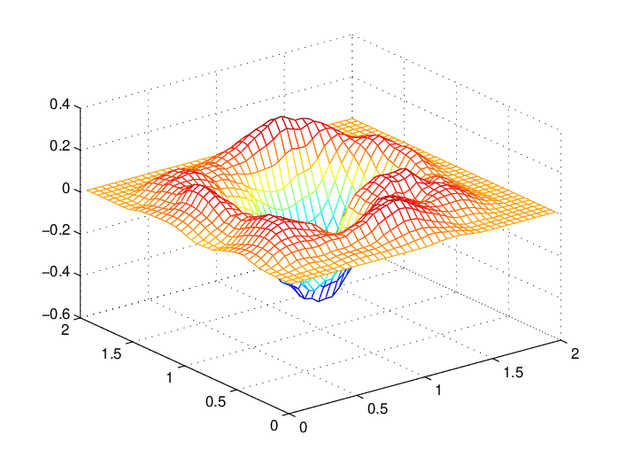
The true density $f$ and its estimate are given in Figure 2 . The difference between the true density and the estimate is plotted in Figure 3. The right plot in Figure 3 shows $f_{nh}^{+-}$ . Clearly this estimate is best in the $+-$ quadrant, as predicted by the theory.

Example 5.2

In our second example $f$ is the density of the random vector $(Y_{1},Y_{2})$ , where $Y_{1}$ and $Y_{2}$ are dependent random variables with a bimodal distribution. The distribution of the vector is a mixture of two distributions like the one in Example 5.1. The values of the $Y$ ’s are generated as follows. With $V_{1}$ and $V_{2}$ having the same distribution as in the previous example the $Y$ values are given by

\begin{pmatrix}Y_{1}\\ Y_{2}\end{pmatrix}=\left\{\begin{array}[]{ll}\begin{pmatrix}V_{1}+0.2\\ V_{2}+0.8\end{pmatrix}&\mbox{, with probability 2/5,}\\ &\\ \begin{pmatrix}V_{1}+0.8\\ V_{2}+0.2\end{pmatrix}&\mbox{, with probability 3/5.}\end{array}\right.

We have simulated 5000 values so $n=5000$ . The bandwidth $h$ , chosen by hand, is equal to $0.35$ .

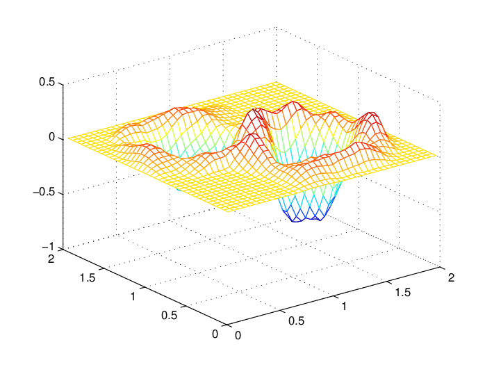
The true density $f$ and its estimate are given in Figure 4 . The difference between the true density and the estimate is plotted in Figure 5. The right plot in Figure 5 shows $f_{nh}^{-+}$ . Clearly this estimate is best in the $-+$ quadrant, as predicted by the theory.

6 Proofs

6.1 Proof of Lemma 2.1

Let us first derive the inversion formulas for $F(x_{1},x_{2})$ . We sum $g(x_{1}-i,x_{2})=F(x_{1}-i,x_{2})-F(x_{1}-i,x_{2}-1)-F(x_{1}-i-1,x_{2})+F(x_{1}-i-1,x_{2}-1)$ over the first coordinate to obtain two telescopic sums. Thus we get

		$\displaystyle\sum_{i=0}^{\infty}g(x_{1}-i,x_{2})$
		$\displaystyle=\sum_{i=0}^{\infty}\{F(x_{1}-i,x_{2})-F(x_{1}-i,x_{2}-1)-F(x_{1}-i-1,x_{2})+F(x_{1}-i-1,x_{2}-1)\}$
		$\displaystyle=\sum_{i=0}^{\infty}\{F(x_{1}-i,x_{2})-F(x_{1}-i-1,x_{2})\}-\sum_{i=0}^{\infty}\{F(x_{1}-i,x_{2}-1)-F(x_{1}-i-1,x_{2}-1)\}$
		$\displaystyle=F(x_{1},x_{2})-F(x_{1},x_{2}-1).$		(40)

Here we used that $\lim_{i\to\infty}F(x_{1}-i,x_{2})=\lim_{i\to\infty}F(x_{1}-i,x_{2}-1)=0$ , for $F$ is a bivariate distribution function. Next, we sum over the second coordinate. Because we also have $\lim_{j\to\infty}F(x_{1},x_{2}-j)=0$ , we get

\sum_{j=0}^{\infty}\sum_{i=0}^{\infty}g(x_{1}-i,x_{2}-j)=\sum_{j=0}^{\infty}\{F(x_{1},x_{2}-j)-F(x_{1},x_{2}-j-1)\}=F(x_{1},x_{2}).

(41)

Because the terms are nonnegative, the order of summation can be interchanged and we have shown (12). Thus we have found an expression for the unobservable probability distribution function $F$ in terms of the observable density function $g$ .

Above, we iterated over $-i$ , so now let us determine what happens when we iterate over $+i$ . First, we write $g(x_{1}+i,x_{2})$ as

g(x_{1}+i,x_{2})=F(x_{1}+i,x_{2})-F(x_{1}+i,x_{2}-1)-F(x_{1}+i-1,x_{2})+F(x_{1}+i-1,x_{2}-1).

(42)

Secondly, we take the sum over the first coordinate. Again we get two telescopic sums. Note that $\lim_{i\to\infty}F(x_{1}+i,x_{2})=F_{Y_{2}}(x_{2})$ and $\lim_{i\to\infty}F(x_{1}+i,x_{2}-1)=F_{Y_{2}}(x_{2}-1)$ , so we get

		$\displaystyle\sum_{i=1}^{\infty}g(x_{1}+i,x_{2})$
		$\displaystyle=\sum_{i=1}^{\infty}\{F(x_{1}+i,x_{2})-F(x_{1}+i,x_{2}-1)-F(x_{1}+i-1,x_{2})+F(x_{1}+i-1,x_{2}-1)\}$
		$\displaystyle=\sum_{i=1}^{\infty}\{F(x_{1}+i,x_{2})-F(x_{1}+i-1,x_{2})\}+\sum_{i=1}^{\infty}\{F(x_{1}+i-1,x_{2}-1)-F(x_{1}+i,x_{2}-1)\}$
		$\displaystyle=F_{Y_{2}}(x_{2})-F(x_{1},x_{2})+F(x_{1},x_{2}-1)-F_{Y_{2}}(x_{2}-1).$		(43)

Thirdly, we sum over the second coordinate. Because $\lim_{j\to\infty}F_{Y_{2}}(x_{2}-j)=0$ , this results in

		$\displaystyle\sum_{j=0}^{\infty}\sum_{i=1}^{\infty}g(x_{1}+i,x_{2}-j)$
		$\displaystyle=\sum_{j=0}^{\infty}\{F_{Y_{2}}(x_{2}-j)-F(x_{1},x_{2}-j)+F(x_{1},x_{2}-j-1)-F_{Y_{2}}(x_{2}-j-1)\}$
		$\displaystyle=\sum_{j=0}^{\infty}\{F_{Y_{2}}(x_{2}-j)-F_{Y_{2}}(x_{2}-j-1)\}-\sum_{j=0}^{\infty}\{F(x_{1},x_{2}-j)-F(x_{1},x_{2}-j-1)\}$
		$\displaystyle=F_{Y_{2}}(x_{2})-F(x_{1},x_{2})=F^{+-}(x_{1},x_{2}).$		(44)

Again, we can interchange the sums and we have shown (14). In similar fashion we can derive (13).

The last formula to recover $F(x_{1},x_{2})$ can be derived as follows. We begin with

g(x_{1}+1,x_{2}+1)=F(x_{1},x_{2})-F(x_{1},x_{2}+1)-F(x_{1}+1,x_{2})+F(x_{1}+1,x_{2}+1).

(45)

Now sum over the first coordinate to obtain

\sum_{i=1}^{\infty}g(x_{1}+i,x_{2}+1)=F(x_{1},x_{2})-F(x_{1},x_{2}+1)-F_{Y_{2}}(x_{2})+F_{Y_{2}}(x_{2}+1).

(46)

Summing over the second coordinate we get

\sum_{j=1}^{\infty}\sum_{i=1}^{\infty}g(x_{1}+i,x_{2}+j)=F(x_{1},x_{2})-F_{Y_{1}}(x_{1})-F_{Y_{2}}(x_{2})+1=F^{++}(x_{1},x_{2}).

(47)

Changing the order of summation again, we obtain $(\ref{++})$ .

The four inversion formulas for $f$ are derived in a similar fashion. From (5) we have

\frac{\partial^{2}}{\partial x_{1}\partial x_{2}}g(x_{1},x_{2})=f(x_{1},x_{2})-f(x_{1},x_{2}-1)-f(x_{1}-1,x_{2})+f(x_{1}-1,x_{2}-1).

Now, following equations (40) and (41), we obtain

\sum_{i=0}^{\infty}\sum_{j=0}^{\infty}\frac{\partial^{2}}{\partial x_{1}\partial x_{2}}g(x_{1}-i,x_{2}-j)=f(x_{1},x_{2}).

(48)

Here we have used $\lim_{x_{1}\to-\infty}f(x_{1},x_{2})=0$ and $\lim_{x_{2}\to-\infty}f(x_{1},x_{2})=0$ .

The other three inversion formulas follow similarly. $\Box$

6.2 Proof of Theorem 3.1

First we consider the estimator $f_{nh}^{++}$ . We have

$\displaystyle{\rm E\,}f_{nh}^{++}$	$\displaystyle(x_{1},x_{2})={\rm E\,}\bigg(\frac{1}{nh^{4}}\sum_{k=1}^{n}\sum_{i=1}^{\infty}\sum_{j=1}^{\infty}w^{\prime}_{1}\bigg(\frac{x_{1}+i-X_{k1}}{h}\bigg)w^{\prime}_{2}\bigg(\frac{x_{2}+j-X_{k2}}{h}\bigg)\bigg)$
	$\displaystyle=\frac{1}{h^{4}}\sum_{i=1}^{\infty}\sum_{j=1}^{\infty}{\rm E\,}w^{\prime}_{1}\bigg(\frac{x_{1}+i-X_{11}}{h}\bigg)w^{\prime}_{2}\bigg(\frac{x_{2}+j-X_{12}}{h}\bigg)$
	$\displaystyle=\frac{1}{h^{4}}\sum_{i=1}^{\infty}\sum_{j=1}^{\infty}\int_{-\infty}^{\infty}\int_{-\infty}^{\infty}w^{\prime}_{1}\Big(\frac{x_{1}+i-u_{1}}{h}\Big)w^{\prime}_{2}\Big(\frac{x_{2}+j-u_{2}}{h}\Big)g(u_{1},u_{2})du_{1}du_{2}.$	(49)

Note that interchanging integrals and sums is allowed because

\frac{1}{h^{4}}\sum_{i=1}^{\infty}\sum_{j=1}^{\infty}\int_{-\infty}^{\infty}\int_{-\infty}^{\infty}\Big|w^{\prime}_{1}\Big(\frac{x_{1}+i-u_{1}}{h}\Big)\Big|\Big|w^{\prime}_{2}\Big(\frac{x_{2}+j-u_{2}}{h}\Big)\Big|g(u_{1},u_{2})du_{1}du_{2}<\infty.

(50)

To check this, we first make the substitutions $v_{1}:=u_{1}-i$ and $v_{2}:=u_{2}-j$ . Secondly, we interchange the sums and integrals again, which is allowed because the integrand is nonnegative (Fubini). We get

		$\displaystyle\frac{1}{h^{4}}\sum_{i=1}^{\infty}\sum_{j=1}^{\infty}\int_{-\infty}^{\infty}\int_{-\infty}^{\infty}\Big\|w^{\prime}_{1}\Big(\frac{x_{1}-v_{1}}{h}\Big)\Big\|\Big\|w^{\prime}_{2}\Big(\frac{x_{2}-v_{2}}{h}\Big)\Big\|g(v_{1}+i,v_{2}+j)dv_{1}dv_{2}$
		$\displaystyle=\frac{1}{h^{4}}\int_{-\infty}^{\infty}\int_{-\infty}^{\infty}\Big\|w^{\prime}_{1}\Big(\frac{x_{1}-v_{1}}{h}\Big)\Big\|\Big\|w^{\prime}_{2}\Big(\frac{x_{2}-v_{2}}{h}\Big)\Big\|\sum_{i=1}^{\infty}\sum_{j=1}^{\infty}g(v_{1}+i,v_{2}+j)dv_{1}dv_{2}.$		(51)

Thirdly, noting that $F^{++}(v_{1},v_{2})=\sum_{i=1}^{\infty}\sum_{j=1}^{\infty}g(v_{1}+i,v_{2}+j)dv_{1}dv_{2}$ and that $F^{++}(v_{1},v_{2})\leq 1$ , we obtain

		$\displaystyle\frac{1}{h^{4}}\int_{-\infty}^{\infty}\int_{-\infty}^{\infty}\Big\|w^{\prime}_{1}\Big(\frac{x_{1}-v_{1}}{h}\Big)\Big\|\Big\|w^{\prime}_{2}\Big(\frac{x_{2}-v_{2}}{h}\Big)\Big\|F^{++}(v_{1},v_{2})dv_{1}dv_{2}$
		$\displaystyle\leq\frac{1}{h^{4}}\int_{-\infty}^{\infty}\int_{-\infty}^{\infty}\Big\|w^{\prime}_{1}\Big(\frac{x_{1}-v_{1}}{h}\Big)\Big\|\Big\|w^{\prime}_{2}\Big(\frac{x_{2}-v_{2}}{h}\Big)\Big\|dv_{1}dv_{2}<\infty.$		(52)

Because $w_{1}^{\prime}$ and $w_{2}^{\prime}$ are bounded functions, and have bounded support, this integral is finite. Thus our use of Fubini’s Theorem is justified. Next we apply partial integration twice, yielding

	$\displaystyle{\rm E\,}f_{nh}^{++}($	$\displaystyle x_{1},x_{2})=\frac{1}{h^{4}}\sum_{i=1}^{\infty}\sum_{j=1}^{\infty}\int_{-\infty}^{\infty}w^{\prime}_{2}\Big(\frac{x_{2}+j-u_{2}}{h}\Big)\Bigg(\int_{-\infty}^{\infty}w^{\prime}_{1}\Big(\frac{x_{1}+i-u_{1}}{h}\Big)g(u_{1},u_{2})du_{1}\Bigg)du_{2}$
		$\displaystyle=-\frac{1}{h^{3}}\sum_{i=1}^{\infty}\sum_{j=1}^{\infty}\int_{-\infty}^{\infty}w^{\prime}_{2}\Big(\frac{x_{2}+j-u_{2}}{h}\Big)\Bigg(\int_{-\infty}^{\infty}w_{1}\Big(\frac{x_{1}+i-u_{1}}{h}\Big)\frac{\partial}{\partial u_{1}}g(u_{1},u_{2})du_{1}\Bigg)du_{2}$
		$\displaystyle=-\frac{1}{h^{3}}\sum_{i=1}^{\infty}\sum_{j=1}^{\infty}\int_{-\infty}^{\infty}w_{1}\Big(\frac{x_{1}+i-u_{1}}{h}\Big)\Bigg(\int_{-\infty}^{\infty}w^{\prime}_{2}\Big(\frac{x_{2}+j-u_{2}}{h}\Big)\frac{\partial}{\partial u_{1}}g(u_{1},u_{2})du_{2}\Bigg)du_{1}$
		$\displaystyle=\frac{1}{h^{2}}\sum_{i=1}^{\infty}\sum_{j=1}^{\infty}\int_{-\infty}^{\infty}\int_{-\infty}^{\infty}w_{1}\Big(\frac{x_{1}+i-u_{1}}{h}\Big)w_{2}\Big(\frac{x_{2}+j-u_{2}}{h}\Big)\frac{\partial^{2}}{\partial u_{1}\partial u_{2}}g(u_{1},u_{2})du_{1}du_{2}.$

By the substitutions $v_{1}:=u_{1}-i$ and $v_{2}:=u_{2}-j$ we get

		$\displaystyle{\rm E\,}f_{nh}^{++}(x_{1},x_{2})$
		$\displaystyle=\frac{1}{h^{2}}\sum_{i=1}^{\infty}\sum_{j=1}^{\infty}\int_{-\infty}^{\infty}\int_{-\infty}^{\infty}w_{1}\Big(\frac{x_{1}-v_{1}}{h}\Big)w_{2}\Big(\frac{x_{2}-v_{2}}{h}\Big)\frac{\partial^{2}}{\partial u_{1}\partial u_{2}}g(v_{1}+i,v_{2}+j)dv_{1}dv_{2}.$		(53)

Now we need to interchange integrals and sums again. Therefore, rewrite the equation above as

		$\displaystyle\sum_{i=1}^{\infty}\sum_{j=1}^{\infty}\int_{-\infty}^{\infty}\int_{-\infty}^{\infty}w_{1}\Big(\frac{x_{1}-v_{1}}{h}\Big)w_{2}\Big(\frac{x_{2}-v_{2}}{h}\Big)\frac{\partial^{2}}{\partial v_{1}\partial v_{2}}g(v_{1}+i,v_{2}+j)dv_{1}dv_{2}$
		$\displaystyle=\lim_{M_{1}\to\infty}\lim_{M_{2}\to\infty}\sum_{i=1}^{M_{1}}\sum_{j=1}^{M_{2}}\int_{-\infty}^{\infty}\int_{-\infty}^{\infty}w_{1}\Big(\frac{x_{1}-v_{1}}{h}\Big)w_{2}\Big(\frac{x_{2}-v_{2}}{h}\Big)\frac{\partial^{2}}{\partial v_{1}\partial v_{2}}g(v_{1}+i,v_{2}+j)dv_{1}dv_{2}$
		$\displaystyle=\lim_{M_{1}\to\infty}\lim_{M_{2}\to\infty}\int_{-\infty}^{\infty}\int_{-\infty}^{\infty}w_{1}\Big(\frac{x_{1}-v_{1}}{h}\Big)w_{2}\Big(\frac{x_{2}-v_{2}}{h}\Big)\sum_{i=1}^{M_{1}}\sum_{j=1}^{M_{1}}\frac{\partial^{2}}{\partial v_{1}\partial v_{2}}g(v_{1}+i,v_{2}+j)dv_{1}dv_{2}.$		(54)

By (42) we have $g(v_{1}+i,v_{2})=F(v_{1}+i,v_{2})-F(v_{1}+i,v_{2}-1)-F(v_{1}+i-1,v_{2})+F(v_{1}+i-1,v_{2}-1)$ , so

\frac{\partial^{2}}{\partial v_{1}\partial v_{2}}g(v_{1}+i,v_{2})=f(v_{1}+i,v_{2})-f(v_{1}+i,v_{2}-1)-f(v_{1}+i-1,v_{2})+f(v_{1}+i-1,v_{2}-1).

Following the summation of (43), we find

		$\displaystyle\sum_{i=1}^{M_{1}}\frac{\partial^{2}}{\partial v_{1}\partial v_{2}}g(v_{1}+i,v_{2})$
		$\displaystyle=\sum_{i=1}^{M_{1}}\{f(v_{1}+i,v_{2})-f(v_{1}+i,v_{2}-1)-f(v_{1}+i-1,v_{2})+f(v_{1}+i-1,v_{2}-1)\}$
		$\displaystyle=\sum_{i=1}^{M_{1}}\{f(v_{1}+i,v_{2})-f(v_{1}+i-1,v_{2})\}+\sum_{i=1}^{M_{1}}\{f(v_{1}+i-1,v_{2}-1)-f(v_{1}+i,v_{2}-1)\}$
		$\displaystyle=f(v_{1}+M_{1},v_{2})-f(v_{1},v_{2})-f(v_{1},v_{2}-1)-f(v_{1}+M_{1},v_{2}-1)$		(55)

and

		$\displaystyle\sum_{j=1}^{M_{2}}\sum_{i=1}^{M_{1}}\frac{\partial^{2}}{\partial v_{1}\partial v_{2}}g(v_{1}+i,v_{2}+j)$
		$\displaystyle=\sum_{j=1}^{M_{2}}\{f(v_{1}+M_{1},v_{2}+j)-f(v_{1},v_{2}+j)-f(v_{1},v_{2}+j-1)-f(v_{1}+M_{1},v_{2}+j-1)\}$
		$\displaystyle=\sum_{j=1}^{M_{2}}\{f(v_{1}+M_{1},v_{2}+j)-f(v_{1}+M_{1},v_{2}+j-1)+\sum_{j=1}^{M_{2}}\{f(v_{1},v_{2}+j-1)-f(v_{1},v_{2}+j)\}$
		$\displaystyle=f(v_{1}+M_{1},v_{2}+M_{2})-f(v_{1}+M_{1},v_{2})+f(v_{1},v_{2})-f(v_{1},v_{2}+M_{2}).$		(56)

Note that this sum is finite for all $v_{1},v_{2}$ , because $f$ is bounded. Also note that changing the order of summation is allowed, because $M_{1},M_{2}<\infty$ . By Lemma 2.1 we have

\lim_{M_{1}\to\infty}\lim_{M_{2}\to\infty}\sum_{i=1}^{M_{1}}\sum_{j=1}^{M_{2}}\frac{\partial^{2}}{\partial v_{1}\partial v_{2}}g(v_{1}+i,v_{2}+j)=f(v_{1},v_{2})<\infty.

(57)

We have assumed that $f$ is bounded, so let $f(v_{1},v_{2})\leq\frac{1}{4}A$ for all $v_{1},v_{2}$ , where $A>0$ is a constant. Observe the following inequality

		$\displaystyle\|f(v_{1}+M_{1},v_{2}+M_{2})-f(v_{1}+M_{1},v_{2})+f(v_{1},v_{2})-f(v_{1},v_{2}+M_{2})\|$
		$\displaystyle\leq\|f(v_{1}+M_{1},v_{2}+M_{2})\|+\|f(v_{1}+M_{1},v_{2})\|+\|f(v_{1},v_{2})\|+\|f(v_{1},v_{2}+M_{2})\|$
		$\displaystyle\leq A,$		(58)

for all $v_{1},v_{2},M_{1}$ , and $M_{2}$ . Note that, because $w_{1}$ and $w_{2}$ are nonnegative, bounded and have bounded support,

\int_{-\infty}^{\infty}\int_{-\infty}^{\infty}w_{1}\Big(\frac{x_{1}-v_{1}}{h}\Big)w_{2}\Big(\frac{x_{2}-v_{2}}{h}\Big)dv_{1}dv_{2}<\infty

(59)

for all $x_{1},x_{2}$ . Thus we can apply the Lebesgue Dominated Convergenge Theorem to (53), and find

		$\displaystyle\lim_{M_{1}\to\infty}\lim_{M_{2}\to\infty}\int_{-\infty}^{\infty}\int_{-\infty}^{\infty}w_{1}\Big(\frac{x_{1}-v_{1}}{h}\Big)w_{2}\Big(\frac{x_{2}-v_{2}}{h}\Big)\sum_{i=1}^{M_{1}}\sum_{j=1}^{M_{2}}\frac{\partial^{2}}{\partial v_{1}\partial v_{2}}g(v_{1}+i,v_{2}+j)dv_{1}dv_{2}$
		$\displaystyle=\int_{-\infty}^{\infty}\int_{-\infty}^{\infty}w_{1}\Big(\frac{x_{1}-v_{1}}{h}\Big)w_{2}\Big(\frac{x_{2}-v_{2}}{h}\Big)\lim_{M_{1}\to\infty}\lim_{M_{2}\to\infty}\sum_{i=1}^{M_{1}}\sum_{j=1}^{M_{2}}\frac{\partial^{2}}{\partial v_{1}\partial v_{2}}g(v_{1}+i,v_{2}+j)dv_{1}dv_{2}$
		$\displaystyle=\int_{-\infty}^{\infty}\int_{-\infty}^{\infty}w_{1}\Big(\frac{x_{1}-v_{1}}{h}\Big)w_{2}\Big(\frac{x_{2}-v_{2}}{h}\Big)f(v_{1},v_{2})dv_{1}dv_{2}.$		(60)

Summarizing we now have

{\rm E\,}f_{nh}^{++}(x_{1},x_{2})=\frac{1}{h^{2}}\int_{-\infty}^{\infty}\int_{-\infty}^{\infty}w_{1}\Big(\frac{x_{1}-v_{1}}{h}\Big)w_{2}\Big(\frac{x_{2}-v_{2}}{h}\Big)f(v_{1},v_{2})dv_{1}dv_{2}.

(61)

Substituting $z_{1}:=\frac{x_{1}-v_{1}}{h}$ and $z_{2}:=\frac{x_{2}-v_{2}}{h}$ we get

{\rm E\,}f_{nh}^{++}(x_{1},x_{2})=\int_{-\infty}^{\infty}\int_{-\infty}^{\infty}w_{1}(z_{1})w_{2}(z_{2})f(x_{1}-hz_{1},x_{2}-hz_{2})dz_{1}dz_{2}.

(62)

Using the multivariate version of Taylor’s theorem derived in Wand and Jones (1995) for this particular application, allows us to rewrite

	$\displaystyle f(x_{1}-hz_{1},$	$\displaystyle x_{2}-hz_{2})=f(x_{1},x_{2})-h(z_{1}f_{1}+z_{2}f_{2})(x_{1},x_{2})$
		$\displaystyle+\frac{1}{2}h^{2}(z_{1}^{2}f_{11}+z_{1}z_{2}(f_{12}+f_{21})+z_{2}^{2}f_{22})(x_{1},x_{2})+o(h^{2}).$

We now obtain

	$\displaystyle{\rm E\,}f_{nh}^{++}(x_{1},x_{2})=$	$\displaystyle\int_{-\infty}^{\infty}\int_{-\infty}^{\infty}w_{1}(z_{1})w_{2}(z_{2})\Big(f(x_{1},x_{2})-h(z_{1}f_{1}+z_{2}f_{2})(x_{1},x_{2})$
		$\displaystyle+\frac{1}{2}h^{2}(z_{1}^{2}f_{11}+z_{1}z_{2}(f_{12}+f_{21})+z_{2}^{2}f_{22})(x_{1},x_{2})+o(h^{2})\Big)dz_{1}dz_{2}$
	$\displaystyle=$	$\displaystyle f(x_{1},x_{2})-hf_{1}(x_{1},x_{2})\int_{-\infty}^{\infty}\int_{-\infty}^{\infty}z_{1}w_{1}(z_{1})w_{2}(z_{2})dz_{1}dz_{2}$
		$\displaystyle-hf_{2}(x_{1},x_{2})\int_{-\infty}^{\infty}\int_{-\infty}^{\infty}z_{2}w_{1}(z_{1})w_{2}(z_{2})dz_{1}dz_{2}$
		$\displaystyle+\frac{1}{2}h^{2}f_{11}(x_{1},x_{2})\int_{-\infty}^{\infty}\int_{-\infty}^{\infty}z_{1}^{2}w_{1}(z_{1})w_{2}(z_{2})dz_{1}dz_{2}$
		$\displaystyle+\frac{1}{2}h^{2}(f_{12}+f_{21})(x_{1},x_{2})\int_{-\infty}^{\infty}\int_{-\infty}^{\infty}z_{1}z_{2}w_{1}(z_{1})w_{2}(z_{2})dz_{1}dz_{2}$
		$\displaystyle+\frac{1}{2}h^{2}f_{22}(x_{1},x_{2})\int_{-\infty}^{\infty}\int_{-\infty}^{\infty}z_{2}^{2}w_{1}(z_{1})w_{2}(z_{2})dz_{1}dz_{2}+o(h^{2})$
	$\displaystyle=$	$\displaystyle f(x_{1},x_{2})+\frac{1}{2}h^{2}\Big(\int_{-\infty}^{\infty}z^{2}w_{1}(z)dzf_{11}(x_{1},x_{2})+\int_{-\infty}^{\infty}z^{2}w_{2}(z)dzf_{22}(x_{1},x_{2})\Big)+o(h^{2}).$

This proves statement (22) of the theorem for this individual estimator.

It is easily seen that

		$\displaystyle{\rm E\,}f^{--}_{nh}(x_{1},x_{2})={\rm E\,}f^{-+}_{nh}(x_{1},x_{2})={\rm E\,}f^{+-}_{nh}(x_{1},x_{2})={\rm E\,}f^{++}_{nh}(x_{1},x_{2})$
		$\displaystyle=f(x_{1},x_{2})+\frac{1}{2}h^{2}\Big(\int_{-\infty}^{\infty}z^{2}w_{1}(z)dzf_{11}(x_{1},x_{2})+\int_{-\infty}^{\infty}z^{2}w_{2}(z)dzf_{22}(x_{1},x_{2})\Big)+o(h^{2})$

and thus

{\rm E\,}f_{nh}^{(t)}(x_{1},x_{2})=f(x_{1},x_{2})+\frac{1}{2}h^{2}\Big(\int_{-\infty}^{\infty}z^{2}w_{1}(z)dzf_{11}(x_{1},x_{2})+\int_{-\infty}^{\infty}z^{2}w_{2}(z)dzf_{22}(x_{1},x_{2})\Big)+o(h^{2}),

proving equation (22).

Next let us derive the asymptotic variance. First, define

U_{kh}^{++}(x_{1},x_{2}):=\frac{1}{h^{4}}\sum_{i=1}^{\infty}\sum_{j=1}^{\infty}w^{\prime}_{1}\bigg(\frac{x_{1}+i-X_{k1}}{h}\bigg)w^{\prime}_{2}\bigg(\frac{x_{2}+j-X_{k2}}{h}\bigg).

(63)

Then $f_{nh}^{++}(x_{1},x_{2})=\frac{1}{n}\sum_{k=1}^{n}U_{kh}^{++}(x_{1},x_{2})$ , and since the terms $U_{kh}^{++}$ are independent,

{\rm Var\,}(f_{nh}^{++}(x_{1},x_{2}))=\frac{1}{n}{\rm Var\,}(U_{1h}^{++}(x_{1},x_{2})).

(64)

Secondly, we will determine the variance of $U_{1h}^{++}(x_{1},x_{2})$ . We have

{\rm Var\,}(U_{1h}^{++}(x_{1},x_{2}))={\rm E\,}U_{1h}^{++}(x_{1},x_{2})^{2}-({\rm E\,}U_{1h}^{++}(x_{1},x_{2}))^{2}.

(65)

Let us begin with determining ${\rm E\,}U_{1h}^{++}(x_{1},x_{2})^{2}$ . Note that, if $h<\frac{1}{2}$ , we have

w^{\prime}_{1}\bigg(\frac{x_{1}+i_{1}-X_{k1}}{h}\bigg)w^{\prime}_{2}\bigg(\frac{x_{2}+i_{2}-X_{k2}}{h}\bigg)w^{\prime}_{1}\bigg(\frac{x_{1}+j_{1}-X_{k1}}{h}\bigg)w^{\prime}_{2}\bigg(\frac{x_{2}+j_{2}-X_{k2}}{h}\bigg)=0

(66)

unless $i_{1}=i_{2}$ and $j_{1}=j_{2}$ , where $i_{1},i_{2},j_{1},j_{2}\in\mathbb{Z}$ . This holds because if $i_{1}\neq i_{2}$ or $j_{1}\neq j_{2}$ , then at least two pairs of arguments in the product (66) are more than distance two apart, rendering the product equal to zero. Thus in the following equation, as $h\to 0$ , only the square products do not vanish and we can write

	$\displaystyle{\rm E\,}U_{1h}^{++}(x_{1},x_{2})^{2}$	$\displaystyle={\rm E\,}\bigg(\frac{1}{h^{4}}\sum_{i=1}^{\infty}\sum_{j=1}^{\infty}w^{\prime}_{1}\bigg(\frac{x_{1}+i-X_{11}}{h}\bigg)w^{\prime}_{2}\bigg(\frac{x_{2}+j-X_{12}}{h}\bigg)\bigg)^{2}$
		$\displaystyle=\frac{1}{h^{8}}\sum_{i=1}^{\infty}\sum_{j=1}^{\infty}{\rm E\,}\bigg(w^{\prime}_{1}\bigg(\frac{x_{1}+i-X_{11}}{h}\bigg)w^{\prime}_{2}\bigg(\frac{x_{2}+j-X_{12}}{h}\bigg)\bigg)^{2}.$

Now we use the substitutions $v_{1}:=u_{1}-i$ and $v_{2}:=u_{2}-j$ to obtain

	$\displaystyle{\rm E\,}U_{1h}^{++}(x_{1},x_{2})^{2}$	$\displaystyle=\frac{1}{h^{8}}\sum_{i=1}^{\infty}\sum_{j=1}^{\infty}\int_{-\infty}^{\infty}\int_{-\infty}^{\infty}\Big(w^{\prime}_{1}\Big(\frac{x_{1}+i-u_{1}}{h}\Big)w^{\prime}_{2}\Big(\frac{x_{2}+j-u_{2}}{h}\Big)\Big)^{2}g(u_{1},u_{2})du_{1}du_{2}$
		$\displaystyle=\frac{1}{h^{8}}\sum_{i=1}^{\infty}\sum_{j=1}^{\infty}\int_{-\infty}^{\infty}\int_{-\infty}^{\infty}\Big(w^{\prime}_{1}\bigg(\frac{x_{1}-v_{1}}{h}\Big)w^{\prime}_{2}\Big(\frac{x_{2}-v_{2}}{h}\Big)\Big)^{2}g(v_{1}+i,v_{2}+j)dv_{1}dv_{2}.$

Note that the integrand is nonnegative, thus interchanging sums and integrals is allowed (Fubini), so

	$\displaystyle{\rm E\,}U_{1h}^{++}(x_{1},x_{2})^{2}$	$\displaystyle=\frac{1}{h^{8}}\int_{-\infty}^{\infty}\int_{-\infty}^{\infty}\Big(w^{\prime}_{1}\Big(\frac{x_{1}-v_{1}}{h}\Big)w^{\prime}_{2}\Big(\frac{x_{2}-v_{2}}{h}\Big)\Big)^{2}\sum_{i=1}^{\infty}\sum_{j=1}^{\infty}g(v_{1}+i,v_{2}+j)dv_{1}dv_{2}$
		$\displaystyle=\frac{1}{h^{8}}\int_{-\infty}^{\infty}\int_{-\infty}^{\infty}w^{\prime}_{1}\Big(\frac{x_{1}-v_{1}}{h}\Big)^{2}w^{\prime}_{2}\Big(\frac{x_{2}-v_{2}}{h}\Big)^{2}F^{++}(v_{1},v_{2})dv_{1}dv_{2}.$

Now apply the substitutions $z_{1}=(x_{1}-v_{1})/h$ and $z_{2}=(x_{2}-v_{2})/h$ and recall the bounded support of $w^{\prime}_{1}$ and $w^{\prime}_{2}$ . Furthermore, because $\lim_{h\to 0}F^{++}(x_{1}-hz_{1},x_{2}-hz_{2})=F^{++}(x_{1},x_{2})\leq 1$ , we can again apply the Lebesgue dominated convergence theorem

	$\displaystyle{\rm E\,}U_{1h}^{++}(x_{1},x_{2})^{2}$	$\displaystyle=\frac{1}{h^{6}}\int_{-1}^{1}\int_{-1}^{1}w^{\prime}_{1}(z_{1})^{2}w^{\prime}_{2}(z_{2})^{2}F^{++}(x_{1}-hz_{1},x_{2}-hz_{2})dz_{1}dz_{2}$
		$\displaystyle=\frac{1}{h^{6}}F^{++}(x_{1},x_{2})\int_{-1}^{1}w^{\prime}_{1}(z_{1})^{2}dz_{1}\int_{-1}^{1}w^{\prime}_{2}(z_{2})^{2}dz_{2}+o(h^{-6}).$		(67)

Now note that ${\rm E\,}U^{++}_{1h}(x_{1},x_{2})={\rm E\,}f^{++}_{nh}(x_{1},x_{2})=f(x_{1},x_{2})+O(h^{2})$ . So

	$\displaystyle{\rm Var\,}(f_{nh}^{++}(x_{1},x_{2}))$	$\displaystyle=\frac{1}{n}{\rm Var\,}(U_{1h}^{++}(x_{1},x_{2}))$
		$\displaystyle=\frac{1}{n}\Big[{\rm E\,}U_{1h}^{++}(x_{1},x_{2})^{2}-({\rm E\,}U_{1h}^{++}(x_{1},x_{2}))^{2}\Big]$
		$\displaystyle=\frac{1}{n}\Bigg[\frac{1}{h^{6}}F^{++}(x_{1},x_{2})\int_{-1}^{1}w^{\prime}_{1}(z_{1})^{2}dz_{1}\int_{-1}^{1}w^{\prime}_{2}(z_{2})^{2}dz_{2}+o(h^{-6})-f(x_{1},x_{2})^{2}-O(h^{2})\Bigg]$
		$\displaystyle=\frac{1}{nh^{6}}F^{++}(x_{1},x_{2})\int_{-1}^{1}w^{\prime}_{1}(z_{1})^{2}dz_{1}\int_{-1}^{1}w^{\prime}_{2}(z_{2})^{2}dz_{2}+o(n^{-1}h^{-6}).$

We can follow a similar procedure to obtain the variances of the other estimators. To summarize we get

		$\displaystyle{\rm Var\,}(f_{nh}^{--}(x_{1},x_{2}))=\frac{1}{nh^{6}}F^{--}(x_{1},x_{2})\int_{-1}^{1}w^{\prime}_{1}(z_{1})^{2}dz_{1}\int_{-1}^{1}w^{\prime}_{2}(z_{2})^{2}dz_{2}+o(n^{-1}h^{-6}),$
		$\displaystyle{\rm Var\,}(f_{nh}^{-+}(x_{1},x_{2}))=\frac{1}{nh^{6}}F^{-+}(x_{1},x_{2})\int_{-1}^{1}w^{\prime}_{1}(z_{1})^{2}dz_{1}\int_{-1}^{1}w^{\prime}_{2}(z_{2})^{2}dz_{2}+o(n^{-1}h^{-6}),$
		$\displaystyle{\rm Var\,}(f_{nh}^{+-}(x_{1},x_{2}))=\frac{1}{nh^{6}}F^{+-}(x_{1},x_{2})\int_{-1}^{1}w^{\prime}_{1}(z_{1})^{2}dz_{1}\int_{-1}^{1}w^{\prime}_{2}(z_{2})^{2}dz_{2}+o(n^{-1}h^{-6}),$
		$\displaystyle{\rm Var\,}(f_{nh}^{++}(x_{1},x_{2}))=\frac{1}{nh^{6}}F^{++}(x_{1},x_{2})\int_{-1}^{1}w^{\prime}_{1}(z_{1})^{2}dz_{1}\int_{-1}^{1}w^{\prime}_{2}(z_{2})^{2}dz_{2}+o(n^{-1}h^{-6}).$

Now let us determine the variance of combinations of these estimators. We have

	$\displaystyle{\rm Var\,}$	$\displaystyle(f_{nh}^{(t)}(x_{1},x_{2}))={\rm Var\,}(t_{1}f^{--}_{nh}(x_{1},x_{2})+t_{2}f^{-+}_{nh}(x_{1},x_{2})+t_{3}f^{+-}_{nh}(x_{1},x_{2})+t_{4}f^{++}_{nh}(x_{1},x_{2}))$
	$\displaystyle=$	$\displaystyle t_{1}^{2}{\rm Var\,}(f^{--}_{nh}(x_{1},x_{2}))+t_{2}^{2}{\rm Var\,}(f^{-+}_{nh}(x_{1},x_{2}))+t_{3}^{2}{\rm Var\,}(f^{+-}_{nh}(x_{1},x_{2}))+t_{4}^{2}{\rm Var\,}(f^{++}_{nh}(x_{1},x_{2}))$
		$\displaystyle+2t_{1}t_{2}{\rm Cov\,}(f^{--}_{nh}(x_{1},x_{2}),f^{-+}_{nh}(x_{1},x_{2}))+2t_{1}t_{3}{\rm Cov\,}(f^{--}_{nh}(x_{1},x_{2}),f^{+-}_{nh}(x_{1},x_{2}))$
		$\displaystyle+2t_{1}t_{4}{\rm Cov\,}(f^{--}_{nh}(x_{1},x_{2}),f^{++}_{nh}(x_{1},x_{2}))+2t_{2}t_{3}{\rm Cov\,}(f^{-+}_{nh}(x_{1},x_{2}),f^{+-}_{nh}(x_{1},x_{2}))$
		$\displaystyle+2t_{2}t_{4}{\rm Cov\,}(f^{-+}_{nh}(x_{1},x_{2}),f^{++}_{nh}(x_{1},x_{2}))+2t_{3}t_{4}{\rm Cov\,}(f^{+-}_{nh}(x_{1},x_{2}),f^{++}_{nh}(x_{1},x_{2})).$

Let us look at ${\rm Cov\,}(f^{--}_{nh}(x_{1},x_{2}),f^{-+}_{nh}(x_{1},x_{2}))$ . In similar fashion as we determined the variance, we find

	$\displaystyle{\rm Cov\,}(f^{--}_{nh}(x_{1},x_{2}),f^{-+}_{nh}(x_{1},x_{2}))$	$\displaystyle=\frac{1}{n}{\rm Cov\,}(U_{1h}^{--}(x_{1},x_{2}),U_{1h}^{-+}(x_{1},x_{2}))$
		$\displaystyle=\frac{1}{n}\big[{\rm E\,}U_{1h}^{--}(x_{1},x_{2})U_{1h}^{-+}(x_{1},x_{2})-{\rm E\,}U_{1h}^{--}(x_{1},x_{2}){\rm E\,}U_{1h}^{-+}(x_{1},x_{2})\big]$

Let us first determine ${\rm E\,}U_{1h}^{--}(x_{1},x_{2})U_{1h}^{-+}(x_{1},x_{2})$ . Note that, if $h<\frac{1}{2}$ , we have

w^{\prime}_{1}\bigg(\frac{x_{1}-i_{1}-X_{k1}}{h}\bigg)w^{\prime}_{2}\bigg(\frac{x_{2}-i_{2}-X_{k2}}{h}\bigg)w^{\prime}_{1}\bigg(\frac{x_{1}-j_{1}-X_{k1}}{h}\bigg)w^{\prime}_{2}\bigg(\frac{x_{2}+j_{2}-X_{k2}}{h}\bigg)=0,

(68)

for all $i_{1},i_{2},j_{1}$ and $j_{2}$ . This holds because the second and fourth argument in the product (68) are always more than distance two apart, rendering the product equal to zero. Thus

{\rm E\,}U_{1h}^{--}(x_{1},x_{2})U_{1h}^{-+}(x_{1},x_{2})=0.

(69)

Secondly, because we have already determined ${\rm E\,}U_{1h}^{--}(x_{1},x_{2})$ and ${\rm E\,}U_{1h}^{-+}(x_{1},x_{2})$ earlier, we know that

{\rm E\,}U_{1h}^{--}(x_{1},x_{2}){\rm E\,}U_{1h}^{-+}(x_{1},x_{2})=f(x_{1},x_{2})^{2}+O(h^{2}).

(70)

Thus

{\rm Cov\,}(f^{--}_{nh}(x_{1},x_{2}),f^{-+}_{nh}(x_{1},x_{2}))=\frac{1}{n}[-f(x_{1},x_{2})^{2}-O(h^{2})]=o(n^{-1}h^{-6}).

(71)

This result holds for all the covariances. So we arrive at

	$\displaystyle{\rm Var\,}(f_{nh}(x_{1},x_{2}))=$	$\displaystyle(t_{1}^{2}F^{--}(x_{1},x_{2})+t_{2}^{2}F^{-+}(x_{1},x_{2})+t_{3}^{2}F^{+-}(x_{1},x_{2})+t_{4}^{2}F^{++}(x_{1},x_{2}))$
		$\displaystyle\frac{1}{nh^{6}}\int_{-1}^{1}w^{\prime}_{1}(z_{1})^{2}dz_{1}\int_{-1}^{1}w^{\prime}_{2}(z_{2})^{2}dz_{2}+o(n^{-1}h^{-6})$
	$\displaystyle=$	$\displaystyle B(x_{1},x_{2},t_{1},t_{2},t_{3},t_{4})\frac{1}{nh^{6}}\int_{-1}^{1}w^{\prime}_{1}(z_{1})^{2}dz_{1}\int_{-1}^{1}w^{\prime}_{2}(z_{2})^{2}dz_{2}+o(n^{-1}h^{-6}).$

This proves statement (23) of the theorem. $\Box$

6.3 Proof of Theorem 4.1

The convex combination of the four density estimators is given by

f_{nh}^{(t)}(x_{1},x_{2})=t_{1}f^{--}_{nh}(x_{1},x_{2})+t_{2}f^{-+}_{nh}(x_{1},x_{2})+t_{3}f^{+-}_{nh}(x_{1},x_{2})+t_{4}f^{++}_{nh}(x_{1},x_{2}),

(72)

where $t_{1}+t_{2}+t_{3}+t_{4}=1$ . Now define

		$\displaystyle S_{1nh}(x_{1},x_{2})=f^{--}_{nh}(x_{1},x_{2})-f^{+-}_{nh}(x_{1},x_{2}),$
		$\displaystyle S_{2nh}(x_{1},x_{2})=-f^{-+}_{nh}(x_{1},x_{2})+f^{++}_{nh}(x_{1},x_{2}),$
		$\displaystyle S_{3nh}(x_{1},x_{2})=f^{--}_{nh}(x_{1},x_{2})-f^{-+}_{nh}(x_{1},x_{2}),$
		$\displaystyle S_{4nh}(x_{1},x_{2})=-f^{+-}_{nh}(x_{1},x_{2})+f^{++}_{nh}(x_{1},x_{2}).$

We can rewrite (72) as

f_{nh}^{(t)}(x_{1},x_{2})=f^{--}_{nh}(x_{1},x_{2})-(t_{3}+t_{4})S_{1nh}(x_{1},x_{2})-t_{2}S_{3nh}(x_{1},x_{2})+t_{4}S_{4nh}(x_{1},x_{2}),

(73)

Lemma 6.1

Under the conditions of Theorem 4.1 we have, for $i=1,\ldots,4$ ,

		$\displaystyle{\rm E\,}S_{inh}(x_{1},x_{2})=0,$		(74)
		$\displaystyle{\rm E\,}S_{inh}(x_{1},x_{2})^{2}=O\Big(\frac{1}{nh^{6}}\Big),$		(75)
		$\displaystyle{\rm E\,}S_{inh}(x_{1},x_{2})^{4}=O\Big(\frac{1}{n^{2}h^{12}}\Big).$		(76)

Proof

We give the proof for $S_{1nh}(x_{1},x_{2})$ . The other claims can be proved similarly.

Note that

	$\displaystyle S_{1nh}(x_{1},x_{2})$	$\displaystyle=f^{--}_{nh}(x_{1},x_{2})-f^{+-}_{nh}(x_{1},x_{2})$
		$\displaystyle=\frac{1}{nh^{4}}\sum_{k=1}^{n}\sum_{i=0}^{\infty}\sum_{j=0}^{\infty}w^{\prime}_{1}(\frac{x_{1}-i-X_{k1}}{h})w^{\prime}_{2}(\frac{x_{2}-j-X_{k2}}{h})$
		$\displaystyle\quad\quad+\frac{1}{nh^{4}}\sum_{k=1}^{n}\sum_{i=1}^{\infty}\sum_{j=0}^{\infty}w^{\prime}_{1}(\frac{x_{1}+i-X_{k1}}{h})w^{\prime}_{2}(\frac{x_{2}-j-X_{k2}}{h})$
		$\displaystyle=\frac{1}{nh^{4}}\sum_{k=1}^{n}\sum_{i=-\infty}^{\infty}\sum_{j=0}^{\infty}w^{\prime}_{1}(\frac{x_{1}-i-X_{k1}}{h})w^{\prime}_{2}(\frac{x_{2}-j-X_{k2}}{h}).$

Define

U_{1kh}(x_{1},x_{2}):=\frac{1}{h^{4}}\sum_{i=-\infty}^{\infty}\sum_{j=1}^{\infty}w^{\prime}_{1}\bigg(\frac{x_{1}+i-X_{k1}}{h}\bigg)w^{\prime}_{2}\bigg(\frac{x_{2}+j-X_{k2}}{h}\bigg).

(77)

Then $S_{1nh}(x_{1},x_{2})=\frac{1}{n}\sum_{k=1}^{n}U_{1kh}(x_{1},x_{2})$ and the terms in the sum are independent.

Following similar steps as in the proof of Theorem 3.1 we get

	$\displaystyle{\rm E\,}U_{1kh}$	$\displaystyle(x_{1},x_{2})=\int_{-\infty}^{\infty}\int_{-\infty}^{\infty}w_{1}\Big(\frac{x_{1}-v_{1}}{h}\Big)w_{2}\Big(\frac{x_{2}-v_{2}}{h}\Big)\frac{\partial^{2}}{\partial v_{1}\partial v_{2}}\sum_{i=-\infty}^{\infty}\sum_{j=1}^{\infty}g(v_{1}+i,v_{2}+j)dv_{1}dv_{2}$
		$\displaystyle=\int_{-\infty}^{\infty}\int_{-\infty}^{\infty}w_{1}\Big(\frac{x_{1}-v_{1}}{h}\Big)w_{2}\Big(\frac{x_{2}-v_{2}}{h}\Big)\frac{\partial^{2}}{\partial v_{1}\partial v_{2}}(1-F_{Y_{2}}(v_{2}))dv_{1}dv_{2}=0.$

We also have, as in the same proof,

{\rm E\,}S_{1nh}(x_{1},x_{2})^{2}=\mathop{\rm Var}\nolimits(S_{1nh}(x_{1},x_{2}))=\frac{1}{n}\,\mathop{\rm Var}\nolimits(U_{11h}(x_{1},x_{2}))=O\Big(\frac{1}{nh^{6}}\Big).

Finally we consider the fourth moment of $S_{1nh}(x_{1},x_{2})=\frac{1}{n}\sum_{k=1}^{n}U_{1kh}(x_{1},x_{2})$ . By independence of the terms we have

	$\displaystyle{\rm E\,}S_{1nh}$	$\displaystyle(x_{1},x_{2})^{4}=\frac{1}{n^{3}}\,{\rm E\,}U_{11h}(x_{1},x_{2})^{4}+\frac{3(n-1)}{n^{3}}\,\Big({\rm E\,}U_{11h}(x_{1},x_{2})^{2}\Big)^{2}$
		$\displaystyle=\frac{1}{n^{3}}\,O\Big(\frac{1}{h^{14}}\Big)+\frac{3(n-1)}{n^{3}}\,\Big(O\Big(\frac{1}{h^{6}}\Big)\Big)^{2}=O\Big(\frac{1}{n^{2}h^{12}}\Big).$

This completes the proof of the lemma. $\Box$

From (73) we get, omitting the arguments $(x_{1},x_{2})$ ,

f_{nh}^{(\hat{t}_{n})}-f_{nh}^{(\bar{t})}=-(\hat{t}_{n3}-\bar{t}_{3})S_{1nh}-(\hat{t}_{n4}-\bar{t}_{4})S_{1nh}-(\hat{t}_{n2}-\bar{t}_{2})S_{3nh}+(\hat{t}_{n4}-\bar{t}_{4})S_{4nh}.

(78)

Hence, under the assumptions of the theorem and by the Cauchy Schwarz inequality, we have

	$\displaystyle{\rm E\,}\|f_{nh}^{(\hat{t}_{n})}$	$\displaystyle-f_{nh}^{(\bar{t})}\|\leq{\rm E\,}\|\hat{t}_{n3}-\bar{t}_{3}\|\|S_{1nh}\|+{\rm E\,}\|\hat{t}_{n4}-\bar{t}_{4}\|\|S_{1nh}\|+{\rm E\,}\|\hat{t}_{n2}-\bar{t}_{2}\|\|S_{3nh}\|+{\rm E\,}\|\hat{t}_{n4}-\bar{t}_{4}\|\|S_{4nh}\|$
		$\displaystyle\leq\Big({\rm E\,}(\hat{t}_{n3}-\bar{t}_{3})^{2}\Big)^{1/2}\Big({\rm E\,}S_{1nh}^{2}\Big)^{1/2}+\Big({\rm E\,}(\hat{t}_{n4}-\bar{t}_{4})^{2}\Big)^{1/2}\Big({\rm E\,}S_{1nh}^{2}\Big)^{1/2}$
		$\displaystyle+\Big({\rm E\,}(\hat{t}_{n2}-\bar{t}_{2})^{2}\Big)^{1/2}\Big({\rm E\,}S_{3nh}^{2}\Big)^{1/2}+\Big({\rm E\,}(\hat{t}_{n4}-\bar{t}_{4})^{2}\Big)^{1/2}\Big({\rm E\,}S_{4nh}^{2}\Big)^{1/2}$
		$\displaystyle=\Big(o(nh^{10})O\Big(\frac{1}{nh^{6}}\Big)\Big)^{1/2}=o(h^{2}).$

Similarly we have, since $(y_{1}+y_{2}+y_{3}+y_{4})^{2}\leq 4(y_{1}^{2}+y_{2}^{2}+y_{3}^{2}+y_{4}^{2})$ ,

	$\displaystyle\mathop{\rm Var}\nolimits(f_{nh}^{(\hat{t}_{n})}$	$\displaystyle-f_{nh}^{(\bar{t})})\leq{\rm E\,}(f_{nh}^{(\hat{t}_{n})}-f_{nh}^{(\bar{t})})^{2}$
		$\displaystyle\leq 4{\rm E\,}(\hat{t}_{n3}-\bar{t}_{3})^{2}S_{1nh}^{2}+4{\rm E\,}(\hat{t}_{n4}-\bar{t}_{4})^{2}S_{1nh}^{2}+4{\rm E\,}(\hat{t}_{n2}-\bar{t}_{2})^{2}S_{3nh}^{2}+4{\rm E\,}(\hat{t}_{n4}-\bar{t}_{4})^{2}S_{4nh}^{2}$
		$\displaystyle\leq 4\Big({\rm E\,}(\hat{t}_{n3}-\bar{t}_{3})^{4}\Big)^{1/2}\Big({\rm E\,}S_{1nh}^{4}\Big)^{1/2}+4\Big({\rm E\,}(\hat{t}_{n4}-\bar{t}_{4})^{4}\Big)^{1/2}\Big({\rm E\,}S_{1nh}^{4}\Big)^{1/2}$
		$\displaystyle+4\Big({\rm E\,}(\hat{t}_{n2}-\bar{t}_{2})^{4}\Big)^{1/2}\Big({\rm E\,}S_{3nh}^{4}\Big)^{1/2}+4\Big({\rm E\,}(\hat{t}_{n4}-\bar{t}_{4})^{4}\Big)^{1/2}\Big({\rm E\,}S_{4nh}^{4}\Big)^{1/2}$
		$\displaystyle=o(1)\Big(O\Big(\frac{1}{n^{2}h^{12}}\Big)\Big)^{1/2}=o\Big(\frac{1}{nh^{6}}\Big).$

Since the two bounds above are negligible compared to the order of the bias and variance in Theorem 3.1 it follows that this theorem also holds for the estimator with estimated weights.

In order to prove asymptotic normality note that by Lemma 6.1 and condition (34) it follows that $\sqrt{n}h^{3}$ times each of the terms in the representation (78) vanish in probability. Also it follows that $\sqrt{n}h^{3}$ times the expectation of (78) vanishes asymptotically. Hence the limit distributions of of $\sqrt{n}h^{3}(f_{nh}^{(\hat{t}_{n})}-{\rm E\,}f_{nh}^{(\hat{t}_{n})})$ and $\sqrt{n}h^{3}(f_{nh}^{(\bar{t})}-{\rm E\,}f_{nh}^{(\bar{t})})$ coincide. The limit distribution of the latter follows by checking the Lyapounov condition for asymptotic normality.

$\Box$

6.4 Proof of lemma 4.3

Proof Let us first introduce some notation. Define the vectors ${\mathbf{v}}(x_{1},x_{2})$ and ${\mathbf{\tilde{v}}}_{n\tilde{h}}(x_{1},x_{2})$ by

		$\displaystyle{\mathbf{v}}(x_{1},x_{2})=(F^{--}(x_{1},x_{2}),F^{-+}(x_{1},x_{2}),F^{+-}(x_{1},x_{2}),F^{++}(x_{1},x_{2})),$
		$\displaystyle{\mathbf{\tilde{v}}}_{n\tilde{h}}(x_{1},x_{2})=({\tilde{F}}_{n\tilde{h}}^{--}(x_{1},x_{2}),{\tilde{F}}_{n\tilde{h}}^{-+}(x_{1},x_{2}),{\tilde{F}}_{n\tilde{h}}^{+-}(x_{1},x_{2}),{\tilde{F}}_{n\tilde{h}}^{++}(x_{1},x_{2})).$

Note that, for $n$ large enough, the components of these vectors are all at least $\epsilon_{n}$ and that they are at most one.

We will only check (29) and (31) for $i$ equal to one. The other cases can be treated similarly. Then we also need the vector of partial derivatives of the the function $\tilde{t}_{1}(y_{1},y_{2},,y_{3},y_{4})$ . Note that on the line segment between ${\mathbf{\tilde{v}}}_{n\tilde{h}}(x_{1},x_{2})$ and ${\mathbf{v}}(x_{1},x_{2})$ all the components are all at least $\epsilon_{n}$ and that they are at most one. This implies after some computation

\|\nabla\tilde{t}_{1}(y_{1},y_{2},,y_{3},y_{4})\|^{2}\leq\frac{B}{\epsilon_{n}^{6}},

for some constant $B$ , for all points $(y_{1},y_{2},,y_{3},y_{4})$ on this line segment.

We can now apply the multivariate mean value theorem and the Cauchy Schwarz inequality to get

	$\displaystyle(\hat{t}_{n1}(x_{1},x_{2})$	$\displaystyle-\bar{t}_{1}(x_{1},x_{2}))^{2}=(\tilde{t}_{1}({\mathbf{\tilde{v}}}_{n\tilde{h}}(x_{1},x_{2}))-\tilde{t}_{1}({\mathbf{v}}(x_{1},x_{2})))^{2}$
		$\displaystyle=({\mathbf{\tilde{v}}}_{n\tilde{h}}(x_{1},x_{2})-{\mathbf{v}}(x_{1},x_{2}))\cdot\nabla\tilde{t}_{1}(y_{1},y_{2},,y_{3},y_{4}))^{2}$
		$\displaystyle\leq\\|{\mathbf{\tilde{v}}}_{n\tilde{h}}(x_{1},x_{2})-{\mathbf{v}}(x_{1},x_{2})\\|^{2}\\|\nabla\tilde{t}_{1}(y_{1},y_{2},,y_{3},y_{4}))\\|^{2}$
		$\displaystyle\leq\frac{B}{\epsilon_{n}^{6}}\,\\|{\mathbf{\tilde{v}}}_{n\tilde{h}}(x_{1},x_{2})-{\mathbf{v}}(x_{1},x_{2})\\|^{2},$

where $(y_{1},y_{2},,y_{3},y_{4})$ is a point on the line segment between ${\mathbf{\tilde{v}}}(x_{1},x_{2})_{n\tilde{h}}$ and ${\mathbf{v}}(x_{1},x_{2})$ . Note that $\|{\mathbf{\tilde{v}}}_{n\tilde{h}}(x_{1},x_{2})-{\mathbf{v}}(x_{1},x_{2})\|^{2}$ is a sum of four terms like $({\tilde{F}}_{n\tilde{h}}^{--}(x_{1},x_{2})-F^{--}(x_{1},x_{2}))^{2}$ , which is smaller than $(F_{n\tilde{h}}^{--}(x_{1},x_{2})-F^{--}(x_{1},x_{2}))^{2}$ , and that ${\rm E\,}(F_{n\tilde{h}}^{--}(x_{1},x_{2})-F^{--}(x_{1},x_{2}))^{2}$ equals the variance plus the squared bias of $F_{n\tilde{h}}^{--}(x_{1},x_{2})$ . By Theorem 4.2 we can bound these to get

{\rm E\,}(\hat{t}_{n1}(x_{1},x_{2})-\bar{t}_{1}(x_{1},x_{2}))^{2}\leq\frac{B}{\epsilon_{n}^{6}}\Big(O\Big(\frac{1}{n\tilde{h}^{2}}\Big)+O(\tilde{h}^{4})\Big)=O(n^{-2/3}(\log n)^{6}),

for a bandwidth $h$ of order $n^{-1/6}$ . This implies that (29) is satisfied.

Let us now check that (31) is satisfied. By an argument similar to the one above it suffices to check if terms like ${\rm E\,}(F_{n\tilde{h}}^{--}(x_{1},x_{2})-F^{--}(x_{1},x_{2}))^{4}$ vanish asymptotically. Write

F_{n\tilde{h}}^{--}(x_{1},x_{2})-F^{--}(x_{1},x_{2})=F_{n\tilde{h}}^{--}(x_{1},x_{2})-{\rm E\,}F_{n\tilde{h}}^{--}(x_{1},x_{2})+{\rm E\,}F_{n\tilde{h}}^{--}(x_{1},x_{2})-F^{--}(x_{1},x_{2}).

By the triangle inequality we have

	$\displaystyle\Big({\rm E\,}(F_{n\tilde{h}}^{--}$	$\displaystyle(x_{1},x_{2})-F^{--}(x_{1},x_{2}))^{4}\Big)^{1/4}\leq$
		$\displaystyle\leq\Big({\rm E\,}(F_{n\tilde{h}}^{--}(x_{1},x_{2})-{\rm E\,}F_{n\tilde{h}}^{--}(x_{1},x_{2}))^{4}\Big)^{1/4}+\Big({\rm E\,}F_{n\tilde{h}}^{--}(x_{1},x_{2})-F^{--}(x_{1},x_{2})\Big).$

So, by $(a+b)^{4}\leq 8(a^{4}+b^{4}),a,b\geq 0$ , we also have

	$\displaystyle{\rm E\,}(F_{n\tilde{h}}^{--}$	$\displaystyle(x_{1},x_{2})-F^{--}(x_{1},x_{2}))^{4}\leq$
		$\displaystyle\leq 8{\rm E\,}(F_{n\tilde{h}}^{--}(x_{1},x_{2})-{\rm E\,}F_{n\tilde{h}}^{--}(x_{1},x_{2}))^{4}+8\Big({\rm E\,}F_{n\tilde{h}}^{--}(x_{1},x_{2})-F^{--}(x_{1},x_{2})\Big)^{4}.$

Since the bias vanishes by Theorem 4.2 it suffices to prove the bound of the lemma for the fourth power of the error.

Recall from the proof of Theorem 4.2 that $F_{n\tilde{h}}^{--}(x_{1},x_{2})=\frac{1}{n}\sum_{k=1}^{n}U_{kh}^{--}(x_{1},x_{2})$ , where

U_{k\tilde{h}}^{--}(x_{1},x_{2}):=\frac{1}{\tilde{h}^{2}}\sum_{i=0}^{\infty}\sum_{j=0}^{\infty}w_{1}\bigg(\frac{x_{1}-i-X_{k1}}{\tilde{h}}\bigg)w_{2}\bigg(\frac{x_{2}-j-X_{k2}}{\tilde{h}}\bigg).

Note that the $U_{k\tilde{h}}^{--}$ are independent. Now write

F_{n\tilde{h}}^{--}(x_{1},x_{2})-{\rm E\,}F_{n\tilde{h}}^{--}(x_{1},x_{2})=\frac{1}{n}\sum_{k=1}^{n}\tilde{U}_{k\tilde{h}}^{--}(x_{1},x_{2}),

where $\tilde{U}_{k\tilde{h}}^{--}(x_{1},x_{2})=U_{k\tilde{h}}^{--}(x_{1},x_{2})-{\rm E\,}U_{k\tilde{h}}^{--}(x_{1},x_{2})$ . Since ${\rm E\,}\tilde{U}_{kh}^{--}(x_{1},x_{2})$ equals zero we have

{\rm E\,}\Big(\frac{1}{n}\sum_{i=1}^{n}\tilde{U}_{k\tilde{h}}^{--}(x_{1},x_{2})\Big)^{4}=\frac{1}{n^{3}}{\rm E\,}\Big(\tilde{U}_{k\tilde{h}}^{--}(x_{1},x_{2})^{4}\Big)+3\,\frac{n-1}{n^{3}}\Big({\rm E\,}\Big(\tilde{U}_{k\tilde{h}}^{--}(x_{1},x_{2})^{2}\Big)\Big)^{2}.

Similar to the derivation of (67) we get

\frac{1}{n^{3}}{\rm E\,}\Big(\tilde{U}_{k\tilde{h}}^{--}(x_{1},x_{2})^{4}\Big)\sim\frac{1}{n^{3}}{\rm E\,}\Big(U_{k\tilde{h}}^{--}(x_{1},x_{2})^{2}\Big)\sim O\Big(\frac{1}{n^{3}\tilde{h}^{4}}\Big)

and

3\,\frac{n-1}{n^{3}}\big({\rm E\,}\Big(\tilde{U}_{k\tilde{h}}^{--}(x_{1},x_{2})^{2}\Big)\Big)^{2}=3\,\frac{n-1}{n^{3}}\big(\mathop{\rm Var}\nolimits(U_{k\tilde{h}}^{--}(x_{1},x_{2}))\Big)^{2}\sim O\Big(\frac{1}{n^{2}\tilde{h}^{4}}\Big).

Under the condition on $\tilde{h}$ in the lemma both terms vanish. This shows that (31) is satisfied as well. Condition (34) follows from condition (31) by the Cauchy-Schwarz inequality. $\Box$

6.5 An inequality

The next lemma can be used to derive the weights that minimize the asymptotic variance of the convex combination of the original for estimators of the density $f$ .

Lemma 6.2

Let $a_{1},\ldots,a_{m}$ be $m$ positive numbers. Then for all positive $t_{1},\ldots,t_{m}$ with $t_{1}+\ldots+t_{m}=1$ we have

a_{1}t_{1}^{2}+\ldots+a_{m}t_{m}^{2}\geq\frac{a_{1}a_{2}\dots a_{m}}{s_{m}(a_{1},\ldots,a_{m})},

(79)

where $s_{m}(a_{1},\ldots,a_{m})$ is defined by

s_{m}(a_{1},\ldots,a_{m})=a_{2}a_{3}\dots a_{m}+\sum_{j=2}^{m-1}a_{1}\dots a_{j-1}a_{j+1}\dots a_{m}+a_{1}a_{2}\dots a_{m-1},

(80)

the sum of the $m$ products of length $m-1$ obtained by skipping one term in the full product.

The minimum is attained at the $t$ vector given by $t_{1}=a_{2}a_{3}\cdots a_{m}/s_{m}(a_{1},\ldots,a_{m})$ and $t_{m}=a_{1}a_{2}\cdots a_{m-1}/s_{m}(a_{1},\ldots,a_{m})$ and

t_{i}=\frac{a_{1}a_{2}\cdots a_{i-1}a_{i+1}\cdots a_{m}}{s_{m}(a_{1},\ldots,a_{m})},\quad i=2,\ldots,m-1.

Proof Introduce the inner product $<\cdot,\cdot>_{a}$ and corresponding norm $\|\cdot\|_{a}$ by

	$\displaystyle<x,y>_{a}$	$\displaystyle=a_{2}a_{3}\dots a_{m}\,x_{1}y_{1}+a_{1}a_{3}\dots a_{m}\,x_{2}y_{2}+\ldots+a_{1}a_{2}\dots a_{m-1}\,x_{m}y_{m},$		(81)
	$\displaystyle\\|x\\|_{a}$	$\displaystyle=\Big(a_{2}a_{3}\dots a_{m}\,x_{1}^{2}+a_{1}a_{3}\dots a_{m}\,x_{2}^{2}+\ldots+a_{1}a_{2}\dots a_{m-1}\,x_{m}^{2}\Big)^{1/2}.$		(82)

Then, with $\mathbf{1}$ equal to the vector of $m$ ones, the Cauchy-Schwarz inequality implies

		$\displaystyle a_{1}a_{2}\dots a_{m}=(a_{1}a_{2}\dots a_{m})(t_{1}+t_{2}+\ldots+t_{m})$
		$\displaystyle=<{\mathbf{1}},(a_{1}t_{1},a_{2}t_{2},\ldots,a_{m}t_{m})>_{a}\ \leq\ \\|1\\|_{a}\\|(a_{1}t_{1},a_{2}t_{2},\ldots,a_{m}t_{m})\\|_{a}$
		$\displaystyle=\sqrt{s(a_{1},\ldots,a_{m})}\Big(a_{2}a_{3}\dots a_{m}\,(a_{1}t_{1})^{2}+a_{1}a_{3}\dots a_{m}\,(a_{2}t_{2})^{2}+\ldots+a_{1}a_{2}\dots a_{m-1}\,(a_{m}t_{m})^{2}\Big)^{1/2}$
		$\displaystyle=\sqrt{s(a_{1},\ldots,a_{m})}\Big((a_{1}a_{2}\dots a_{m})(a_{1}t_{1}^{2}+a_{2}t_{2}^{2}+\ldots+a_{m}t_{m}^{2})\Big)^{1/2},$

which implies the inequality after some rewriting. $\Box$

References

[1] M. Benešová, B. van Es and P. Tegelaar. Bivariate uniform deconvolution. Preprint, ArXiv:1101.0935, 2011.
[2] A. Delaigle and A. Meister. Nonparametric function estimation under Fourier-oscillating noise. Statistica Sinica. To appear, 2011.
[3] S. Donauer, P. Groeneboom and G. Jongbloed. Global rate results for the MLE in a class of deconvolution models. Statist. Probab. Lett. 79: 519–524, 2009.
[4] B. van Es. Combining kernel estimators in the uniform deconvolution model. To appear in Statist. Neerlandica, 2011.
[5] A.J. van Es and A.R. Kok. Simple kernel estimators for certain nonparametric deconvolution problems. Statist. Probab. Lett., 39:151–160, 1998.
[6] A.J. van Es and M.C.A. van Zuijlen. Convex minorant estimators in nonparametric deconvolution problems. Scand. J. Statist. 23: 85–104, 1996.
[7] A. Feuerverger, P.T. Kim and J. Sun. On optimal uniform deconvolution. J. Stat. Theory Pract. 3: 433–451, 2008.
[8] P. Groeneboom and G. Jongbloed. Density estimation in the uniform deconvolution model. Statist. Neerlandica 57: 136–157, 2003.
[9] P. Groeneboom and J.A. Wellner. Information Bounds and Nonparametric Maximum Likelihood. Birkhäuser, Basel, 1992.
[10] P. Hall and A. Meister. A ridge-parameter approach to deconvolution. Ann. Statist., 35: 1535–1558, 2007.
[11] Y. Hu and G. Ridder. Estimation of nonlinear models with measurement error using marginal information. Econometric Society North American Summer Meetings 21, Econometric Society. available at http://ideas.repec.org/p/ecm/nasm04/21.html, 2004.
[12] A. Meister. Deconvolution from Fourier-oscillating error densities under decay and smoothness conditions. Inverse Problems., 24: 015003, 2008.
[13] B.W. Silverman. Density Estimation for Statistics and Data Analysis. Chapman and Hall, London, 1986.
[14] M.P. Wand. Fast computation of multivariate kernel estimators. J. Comput. Graph. Statist., 3: 433–445, 1994.
[15] M.P. Wand and M.C. Jones. Kernel Smoothing. Chapman and Hall, London, 1995.
[16] E. Youndjé and M. Wells. Optimal bandwidth selection for multivariate kernel deconvolution density estimation. Test, 17: 138–162, 2008.