Bending Fuchsian representations of fundamental groups of cusped surfaces in PU(2,1).

Pierre WILL Affiliation: Institut Fourier Affiliation: 100 rue des Maths Affiliation: 38402 St Martin d’Hères Affiliation: France Email: pierre.will@ujf-grenoble.fr

Abstract

We describe a new family of representations of $\pi_{1}(\Sigma)$ in PU(2,1), where $\Sigma$ is a hyperbolic Riemann surface with at least one deleted point. This family is obtained by a bending process associated to an ideal triangulation of $\Sigma$ . We give an explicit description of this family by describing a coordinates system in the spirit of shear coordinates on the Teichmüller space. We identify within this family new examples of discrete, faithful and type-preserving representations of $\pi_{1}(\Sigma)$ . In turn, we obtain a 1-parameter family of embeddings of the Teichmüller space of $\Sigma$ in the PU(2,1)-representation variety of $\pi_{1}(\Sigma)$ . These results generalise to arbitrary $\Sigma$ the results obtained in [42] for the 1-punctured torus.

Key words: Complex hyperbolic geometry, representations of surface groups, Teichmüller space, deformation.

AMS classification 51M10, 32M15, 22E40

1 Introduction

Let $\Sigma$ be an oriented surface with negative Euler characteristic. Describing the representation variety of the fundamental group $\pi_{1}(\Sigma)$ in a given Lie group $G$ has been a major problem during the last two decades. The central object in this field is the character variety

\mbox{Rep${}_{\pi_{1}(\Sigma),G}$ }={\rm Hom}(\pi_{1}(\Sigma),G)//G.

(1)

This problem finds its source in the study of the Teichmüller space of $\Sigma$ , which classifies hyperbolic metrics or complex structures on $\Sigma$ . Riemann’s uniformization theorem implies that the Teichmüller space of $\Sigma$ may be seen as the subset of Rep ${}_{\pi_{1}(\Sigma),{\rm PSL}(2,\mathbb{R})}$ consisting of conjugacy classes of discrete, faithful and type-preserving representations. In the case where $\Sigma$ is closed without boundary, Goldman classified in [17] the connected components of Rep ${}_{\pi_{1}(\Sigma),{\rm PSL}(2,\mathbb{R})}$ using the Euler number of a representation. It turns out that the extremal values of the Euler number correspond to two connected components of Rep ${}_{\pi_{1}(\Sigma),{\rm PSL}(2,\mathbb{R})}$ which are copies of the Teichmüller space of $\Sigma$ . Since then, the question of classifying the connected components of Rep ${}_{\pi_{1}(\Sigma),G}$ , and understanding the situation of dicrete and faithful representations has been addressed for many Lie groups (see for instance [5, 6, 14, 25, 29]). This led to what is sometimes called higher Teichmüller theory. The goal of this work is to present an explicit family of geometrically well-understood representations of the fundamental group of a cusped surface in PU(2,1), the group of holomorphic isometries of the complex hyperbolic plane $\mathbb{H}^{2}_{\mathbb{C}}$ .

In the specific context of PU( $n$ ,1) and complex hyperbolic geometry, the study of representations of surface groups has been initiated by Goldman and Toledo among others ([20, 16, 40]). Since then, the question of the classification of connected components of Rep ${}_{\pi_{1}(\Sigma),{\rm PU(2,1)}}$ has been answered thanks to Toledo’s invariant (see [40, 44]). This invariant is defined as the integral over $\Sigma$ of the pull-back of the Kähler form on $\mathbb{H}^{2}_{\mathbb{C}}$ by a $\rho$ -equivariant embedding of $\tilde{\Sigma}$ into $\mathbb{H}^{2}_{\mathbb{C}}$ . We will denote it by $\textbf{tol}(\rho)$ . If $\Sigma$ is compact without boundary, the Toledo invariant enjoys the following properties.

•

tol is a continuous function of $\rho$ .
•

$\forall\rho\in\,$ Rep ${}_{\pi_{1}(\Sigma),{\rm PU(2,1)}}$ , $\textbf{tol}(\rho)\in 2/3\mathbb{Z}$ .
•

tol satisfies a Milnor-Wood inequality: $|\textbf{tol}(\rho)|\leqslant-4\pi\chi(\Sigma)$ .

Xia proved in [44] that two representations having the same Toledo invariant lie in the same connected component of Rep ${}_{\pi_{1}(\Sigma),{\rm PU(2,1)}}$ , and thus the Toledo invariant classifies connected components of Rep ${}_{\pi_{1}(\Sigma),{\rm PU(2,1)}}$ . Extremal values of the Toledo invariant characterizes those representations preserving a complex line on which they act properly discontinuously (see [20, 40]). These results gave rise to considerable generalisations, from the context of complex hyperbolic space to the wider frame of Hermitian symmetric spaces (see for instance [5, 6, 27, 28]).

The question of discreteness of representations of surface groups in PU( $n$ ,1) is still far from being given a complete answer. It is known for instance that contrary to the case of PSL(2, $\mathbb{R}$ ), discrete and faithful representations are not contained in specific components of Rep_Σ,PU(2,1), as shown for instance in [19] or [1, 2, 15].

This work is concerned with representations of fundamental groups of cusped surfaces. In this case, the Toledo invariant is defined for type-preserving representation (that is, representations mapping classes of loops around punctures to parabolics), but it does not classify the topological components of Rep ${}_{\pi_{1}(\Sigma),{\rm PU(2,1)}}$ , as shown in [24]. The question of the discreteness for such groups has been addressed in several works, see for example [9, 10, 21, 23, 24, 36, 37, 38, 42].

A classical way to produce non-trivial examples of representations of surface groups in PU(2,1) is to start with a representation $\rho_{0}$ preserving a totally geodesic subspace $V$ of $\mathbb{H}^{2}_{\mathbb{C}}$ and to deform it. There are a priori two ways to do so in our case since there are two kinds of maximal totally geodesic subspaces in $\mathbb{H}^{2}_{\mathbb{C}}$ , namely complex lines and totally geodesic Lagrangian planes, or real planes. Complex lines are embeddings of $\mathbb{H}^{1}_{\mathbb{C}}$ with sectional curvature $-1$ , and real planes are embeddings of $\mathbb{H}^{2}_{\mathbb{R}}$ with sectional curvature $-1/4$ . Their respective stabilisers are P(U(1,1) $\times$ U(1)) and PO(2,1) (see for instance [18]). A discrete and faithful representation preserving a complex line (resp. a real plane) is called $\mathbb{C}$ -Fuchsian (resp. $\mathbb{R}$ -Fuchsian). The rigidity results for $\mathbb{C}$ -Fuchsian representations in the case of compact surfaces are no longer true for $\mathbb{R}$ -Fuchsian representation see [22, 32].

The purpose of this work is twofold.

1.

We first describe a family of representations obtained by a bending process. They arise as holonomies of equivariant mappings from the Farey set of a surface $\Sigma$ to the boundary of $\mathbb{H}^{2}_{\mathbb{C}}$ . Roughly speaking, we are bending along the edges of an ideal triangulation of $\Sigma$ , and the case were the representation is $\mathbb{R}$ -Fuchsian corresponds to vanishing bending angles (Theorem 1).
2.

We identify within this family of examples a subfamily of discrete, faithful, and type-preserving representations (Theorem 2). The proof of discreteness is done by showing that the action of $\rho(\pi_{1})$ on $\mathbb{H}^{2}_{\mathbb{C}}$ is discontinuous. We obtain in turn a 1-parameter family of embeddings of the Teichmüller space of $\Sigma$ into Rep ${}_{\pi_{1}(\Sigma),{\rm PU(2,1)}}$ containing only classes of discrete, faithful representations with unipotent boundary holonomy (Theorem 4).

In the context of $\mathbb{H}^{2}_{\mathbb{C}}$ , deformations by bending were first described by Apanasov in [3]. More recently, in [35], Platis has described a complex hyperbolic version of Thurston’s quakebending deformations for deformations of $\mathbb{R}$ -Fuchsian representations of groups in the case of closed surfaces without boundary. If $\rho_{0}$ is an $\mathbb{R}$ -Fuchsian representation of $\pi_{1}(\Sigma)$ and $\Lambda$ is a finite geodesic lamination with a complex transverse measure $\mu$ , Platis shows that there exists $\epsilon>0$ such that any quakebend deformation $\rho_{t\mu}$ of $\rho_{0}$ is complex hyperbolic quasi-Fuchsian for all $t<\epsilon$ . The proof of discreteness in [35] rests on the main result in [32] where the proof of discreteness is done by building a fundamental domain.

In order to sum up our work, let us introduce a little notation.

Throughout this work, we denote by $\Sigma$ a oriented surface of genus $g$ with $n>0$ deleted points, which we denote by $x_{1},\cdots x_{n}$ . We assume that $\Sigma$ has negative Euler characteristic, that is, $2-2g-n<0$ . We denote by $\pi_{1}(\Sigma)$ the fundamental group of $\Sigma$ . It admits the following presentation

\pi_{1}(\Sigma)\sim\langle a_{1},b_{2},\cdots a_{g},b_{g},c_{1}\cdots c_{n}\lvert\prod[a_{i},b_{i}]\prod c_{j}=1\rangle,

where the $c_{j}$ ’s are the homotopy classes of simple loops enclosing the punctures $x_{j}$ of $\Sigma$ . The universal cover of $\Sigma$ is an open disc $\tilde{\Sigma}$ , with a $\pi_{1}$ -invariant family of points on its boundary corresponding to the deleted points of $\Sigma$ . This set of boundary points is called the Farey set of $\Sigma$ , and denoted by $\mathcal{F}_{\infty}$ . If one fixes a finite area hyperbolic structure on $\Sigma$ , the Farey set consists of the fixed points of parabolic elements representing homotopy classes of loops around punctures. In particular, if the holonomy of this hyperbolic structure has its image in PSL(2, $\mathbb{Z}$ ), one recovers this way the usual Farey set $\mathbb{Q}\cup\infty$ .

The idea of shear coordinates on the Teichmüller space of a cusped surface goes back to the eighties with Thurston [39], Bonahon [4] and Penner [34]. The principle is the following. In order to build a hyperbolic structure on a cusped surface $\Sigma$ , it suffices to glue together ideal triangles in the upper half plane. Since there is a unique ideal triangle up to the action of PSL(2, $\mathbb{R}$ ), the only gluing invariant is the cross ratio of the four boundary points associated to a pair of adjacent triangles, which measures the shearing of the two triangles. It is therefore very natural to parametrize structures by decorating triangulations, using (positive) real numbers that should be interpreted as cross ratios. In particular, Penner defined the decorated Teichmüller space of a punctured surface in [34], and gave a description of it in this way. Later, these ideas were successfully exploited and generalised by Fock and Goncharov to study representations of cusped surfaces in real split Lie groups (see [14, 13, 12]). It is possible to give an efficient combinatorial description of a representant of the class of representation of $\pi_{1}(\Sigma)$ associated to a given decoration (see for instance [13]), which we are going to adapt to our context (section 4.3).

As shown in [30], it is possible to describe a similar system of explicit coordinates on an open subset of Rep ${}_{\pi_{1}(\Sigma),{\rm PU(2,1)}}$ which contains all the classes of discrete and faithful representations. However, identifying those classes of representations that are indeed discrete remains out of reach. Therefore, we restrict ourselves to a family of representations obtained by making an additional geometric assumption. More precisely, our first goal is to classify what we call $T$ -bent realizations of $\mathcal{F}_{\infty}$ in $\mathbb{H}^{2}_{\mathbb{C}}$ , where $T$ is an ideal triangulation of $\Sigma$ , that is pairs $(\phi,\rho)$ , where

•

$\rho$ is a representation $\pi_{1}(\Sigma)\longrightarrow$ Isom( $\mathbb{H}^{2}_{\mathbb{C}}$ ),
•

$\phi:\mathcal{F}_{\infty}\longrightarrow\partial\mathbb{H}^{2}_{\mathbb{C}}$ is a $(\pi_{1},\rho)$ -equivariant mapping,
•

for any face $\Delta$ of $\hat{T}$ with vertices $a,b,c\in\mathcal{F}_{\infty}$ , the three points $\phi(a)$ , $\phi(b)$ and $\phi(c)$ form a real ideal triangle of $\mathbb{H}^{2}_{\mathbb{C}}$ , that is, they belong to the boundary of a real plane of $\mathbb{H}^{2}_{\mathbb{C}}$ .

It is natural to use this formalism because of the following remark. Consider a hyperbolic structure on $\Sigma$ with holonomy $\Gamma$ a subgroup of PSL(2, $\mathbb{Z}$ ). Each point of the Farey set $\mathbb{Q}\cup\infty$ is the fixed point of a unique primitive parabolic element of $\Gamma$ , corresponding to a peripheral loop. Now taking $\Gamma$ as a Fuchsian model for $\pi_{1}(\Sigma)$ , any other finite area hyperbolic structure on $\Sigma$ gives rise to a discrete, faithful and type preserving representation $\rho:\Gamma\longrightarrow\mbox{\rm PSL(2,$\mathbb{R}$)}$ . One associates to $\rho$ an equivariant mapping $\phi:\mathcal{F}_{\infty}\longrightarrow\partial\mathbb{H}^{1}_{\mathbb{C}}$ by sending any point $m$ in the Farey set corresponding to the fixed point of the primitive parabolic $p$ to the fixed point of $\rho(p)$ (see also section 6.2).

In order to parametrize these bent realizations, we need a gluing invariant for pairs of real ideal triangles in $\mathbb{H}^{2}_{\mathbb{C}}$ . In the context of PSL(2, $\mathbb{R}$ ), this invariant is the cross-ratio: the unique invariant of a pair of ideal triangles of $\mathbb{H}^{1}_{\mathbb{C}}$ sharing an edge. In the complex hyperbolic context, a pair of real ideal triangles sharing an edge in $\mathbb{H}^{2}_{\mathbb{C}}$ is determined up to holomorphic isometry by a single complex number $\texttt{Z}(\tau_{1},\tau_{2})\in\mathbb{C}\setminus\{-1,0\}$ . This Z-invariant is similar to the Korányi-Reimann cross-ratio on the Heisenberg group (see [18, 26, 43] and remark 9 in section 3.2). Note that Z is an invariant of ordered pairs of real ideal triangles, in the sense that

\texttt{Z}(\tau_{2},\tau_{1})=\overline{\texttt{Z}(\tau_{1},\tau_{2})}.

(2)

This invariant was first used by Falbel in [8] to glue ideal tetrahedra in $\mathbb{H}^{2}_{\mathbb{C}}$ . Falbel needs two such parameters to describe the isometry class of an ideal tetrahedron. We only need one since we only consider pairs of real ideal triangles, which correspond in his terminology to the particular case of symmetric tetrahedra (see section 4.3 of [8]).

The modulus of Z is similar to the cross-ratio in $\mathbb{H}^{1}_{\mathbb{C}}$ : it measures the shearing between two real ideal triangles. Its argument is the bending parameter, which can be seen as the measure of an angle between real planes. In particular, if Z is real, the two adjacent real ideal triangles are contained in a common real plane. We will therefore call a bending decoration of $T$ any application ${\tt D}:e(T)\longrightarrow\mathbb{C}\setminus\{-1,0\}$ (the two cases where $z=0$ or $z=-1$ correspond to degenerate triangles).

As in the case of PSL(2, $\mathbb{R}$ ), it is possible to associate $T$ -bent realizations to bending decorations and we obtain an explicit expression for the images of classes of loops by $\rho$ . We do this in the same spirit as in [13]. Once an ideal triangulation of $\Sigma$ is chosen, any element $\gamma$ of $\pi_{1}(\Sigma)$ can be represented by a sequence of edges of the modified dual graph (see Definition 8). Using the decoration, we associate to each edge of this graph an elementary isometry, and the image of $\gamma$ by $\rho$ is the product of the corresponding elementary isometry. These elementary isometries are either elliptic elements of order 3, or antiholomorphic involutions. The latter appear as the unique isometries exchanging two real ideal triangles with a common edge. They have to be antiholomorphic because of relation (2). As a consequence the image of a homotopy class by $\rho$ is not always holomorphic. This is why the representation $\rho$ is taken in Isom( $\mathbb{H}^{2}_{\mathbb{C}}$ ) rather than in PU(2,1), which is the index two subgroup of Isom( $\mathbb{H}^{2}_{\mathbb{C}}$ ) containing holomorphic isometries. However, for some special triangulations, the image of the representation is in fact contained in PU(2,1). Namely, we show in section 4.4, that the representation $\rho$ associated to a $T$ -bent realization of $\mathcal{F}_{\infty}$ is holomorphic if and only if $T$ is bipartite, that is if its dual graph is bipartite . Now, any cusped surface $\Sigma$ admits a bipartite ideal triangulation (Proposition 11). This bending process produces thus representations of $\pi_{1}(\Sigma)$ in PU(2,1) for any non compact $\Sigma$ . Let us denote by $\mathcal{BD}_{T}$ the set of bending decorations of an ideal triangulation $T$ and by $\mathcal{BR}^{*}_{T}$ the quotient of $\mathcal{BD}_{T}$ by the action of complex conjugation. The first result of our work is the following.

Theorem 1 (Bending Theorem).

There is a bijection between $\mathcal{BD}^{*}_{T}$ and $\mathcal{BR}_{T}$ .

More precisely, we associate to any bending decoration a pair $(r_{1},r_{2})$ of PU(2,1)-classes of bent realizations of $\mathcal{F}_{\infty}$ , which represent the same Isom( $\mathbb{H}^{2}_{\mathbb{C}}$ )-class of realization. The complex conjugation of bending representations corresponds to the permutation $(r_{1},r_{2})\longrightarrow(r_{2},r_{1})$ . This result is proved in section 4.2.

After having classified $T$ -bent realizations, we focus on a special kind: those $T$ -bent realizations corresponding to regular bending decorations, that is decorations of the form ${\tt D}={\tt d}e^{i\theta}$ , where ${\tt d}$ is a positive decoration of $T$ , and $\theta\in]-\pi,\pi]$ is a fixed real number. When $\theta=0$ , we obtain $T$ -bent realizations where all the images of the points of $\mathcal{F}_{\infty}$ are contained in a real plane. The corresponding representations are $\mathbb{R}$ -Fuchsian.

If $c$ is a class of peripheral loop on $\Sigma$ the parabolicity of $\rho(c)$ is simply expressed in terms of the decoration. If $x$ is the puncture of $\Sigma$ surrounded by $c$ , and $e_{1},\cdots,e_{n}$ are the edges of $T$ adjacent to $x$ , the isometry $\rho(c)$ is parabolic if and only if the product $\prod{\tt D}(e_{i})$ has modulus 1. Such a decoration ${\tt D}$ is said to be balanced at $x$ (see section 4.5).

We now state the main result of our work.

Theorem 2 (Discreteness Theorem).

Let $T$ be a bipartite ideal triangulation of $\Sigma$ , $\theta\in]-\pi,\pi[$ be a real number and ${\tt D}$ be a regular bending decoration of $T$ with angular part equal to $\theta$ . Let $\rho$ be a representative of the (unique) Isom( $\mathbb{H}^{2}_{\mathbb{C}}$ )-class of representations associated to ${\tt D}$ . Then

1.

For any index $i$ , $\rho(c_{i})$ is parabolic if and only if ${\tt D}$ is balanced at $x_{i}$ .
2.

The representation $\rho$ does not preserve any totally geodesic subspace of $\mathbb{H}^{2}_{\mathbb{C}}$ , unless $\theta=0$ , in which case it is $\mathbb{R}$ -Fuchsian.
3.

As long as $\theta\in[-\pi/2,\pi/2]$ , the representation $\rho$ is discrete and faithful.

The bending and discreteness theorems are generalisations to the case of any punctured surface of results obtained in [42] in the case of the punctured torus.

If we restrict this result to those decorations ${\tt D}$ which are balanced at every puncture, we obtain a 1-parameter family of embeddings of the Teichmüller space of $\Sigma$ in Rep ${}_{\pi_{1}(\Sigma),{\rm PU(2,1)}}$ $\pi_{1}(\Sigma)$ . The images of these embedding contain only classes of discrete, faithful and type-preserving representations, parametrised by $\theta\in[-\pi/2,\pi/2]$ . Note that the family of embeddings obtained depends on the initial choice of the triangulation.

The proof of Theorem 2 goes as follows. From a bending decoration, we construct a family of real ideal triangles on which $\rho(\pi_{1})$ acts because of the equivariance condition. Under the hypotheses of Theorem 2,we are able to define for each pair $(\tau,\tau^{\prime})$ of real ideal triangles a canonical real hypersurface of $\mathbb{H}^{2}_{\mathbb{C}}$ called the splitting surface of $\tau$ and $\tau^{\prime}$ and denoted by Spl $(\tau,\tau^{\prime})$ . The main steps of the proof consist in proving the following properties for these hypersurfaces.

1.

The splitting surface Spl $(\tau,\tau^{\prime})$ separates $\mathbb{H}^{2}_{\mathbb{C}}$ in two connected components, each of which contains one of $\tau$ and $\tau^{\prime}$ (Proposition 16).
2.

If $\tau$ is surrounded by three real ideal triangles $\tau_{1}$ , $\tau_{2}$ and $\tau_{3}$ , the three splitting surfaces Spl $(\tau,\tau_{i})$ are mutually disjoint (Theorem 3).

It is a direct consequence of these facts that all the constructed triangles are disjoint, and $\rho(\pi_{1}(\Sigma))$ acts discontinuously on their union, and is therefore discrete. The union of all the triangles constructed is a piecewise totally geodesic disc.

Splitting surfaces are examples of spinal $\mathbb{R}$ -surfaces (see section 5.2), which are the inverse images of geodesics by the orthogonal projection on real planes. This terminology refers to Mostow’s spinal surfaces, defined in [31], which are the inverse images of geodesic by the orthogonal projection on a complex line (spinal surfaces are often called bisectors, see [18]). Spinal $\mathbb{R}$ -surfaces appeared first in [42] under the name of $\mathbb{R}$ -balls. They were generalised and used by Parker and Platis in [32] (see also [33]) under the name of packs. In their terminology, spinal $\mathbb{R}$ -surfaces are flat packs. In particular, the characterisation of spinal $\mathbb{R}$ -surfaces given in the Lemma 5 is similar to their definition of packs.

If $\Sigma$ has genus $g$ and $n$ punctures, any ideal triangulation of $\Sigma$ has $6g-6+3n$ edges. The set of conjugacy classes discrete and faithul representations of $\pi_{1}(\Sigma)$ (resp. the Teichmüller space of $\Sigma$ ) has (real) dimension $6g-6+3n$ (resp. $6g-6+2n$ ). The representation variety Rep ${}_{\pi_{1}(\Sigma),{\rm PU(2,1)}}$ has real dimension $16g-16+8n$ , and its subset containing the classes of type preserving representations has real dimension $16g-16+7n$ . If $T$ is an ideal triangulation of $\Sigma$ , $\mathcal{BR}_{T}$ and $\mathcal{BR}^{*}_{T}$ have real dimension $12g-12+6n$ , and may be seen respectively as $\left(\mathbb{C}\setminus\{-1,0\}\right)^{6g-6+3n}$ and its quotient by the action of the complex conjugation. The real dimension of the family of the classes of discrete and faithful representations obtained by examining regular bending decorations of $T$ is $6g-6+3n+1$ and falls to $6g-6+2n+1$ if we add the condition of type-preservation. The Toledo invariant ${\bf tol}$ (see [24, 40]) of a representation is defined for representations of fundamental groups of compact surfaces, and for type preserving representations of surfaces with deleted points. All type-preserving representations we obtain here have vanishing Toledo invariant. This follows from the fact that the representations are constructed from families of real ideal triangles (see section 6).

Our work is organised as follows. We provide in section 2 the necessary background about the complex hyperbolic plane and its isometries. The invariant of a pair of real ideal triangles is described in section 3. Section 4 is devoted to the proof of Theorem 1.We provide in 4.3 the explicit form of the corresponding representations. The characterisation of bent realization giving representations in PU(2,1) in terms of bipartite triangulations is given in 4.4, and we study the holonomy of loops around deleted points in 4.5. We turn then to the proof of Theorem 5. Spinal $\mathbb{R}$ -surfaces and splitting surfaces surfaces are defined and studied in 5.2, and we prove the discreteness part of Theorem 2 in 5.3. Section 6 is devoted to some remarks and comments. In particular, give a quick presentation of the similar classical construction for PSL(2, $\mathbb{R}$ ), and prove Theorem 4.We draw the connection between our work and the previously known families of examples studied in [9, 24, 42].

Acknowledgements

I would like to thank Nicolas Bergeron, Julien Marché and Anne Parreau for fruitful discussions, and John Parker for a useful hint about Proposition 11. Part of this work was carried out during a stay at the Max Planck Institut für Mathematik in Bonn, and I would like to thank the institution for the wonderful working conditions I had there. I thank the referees for their help to improve this work. Last but not least, I thank Elisha Falbel for his constant interest and support.

2 The complex hyperbolic 2-space

We refer the reader to [7, 18] for more precise information and more references about the material exposed in this section.

2.1 $\mathbb{H}^{2}_{\mathbb{C}}$ and its isometries

Let $\mathbb{C}^{2,1}$ denote the vector space $\mathbb{C}^{3}$ equipped with the Hermitian form of signature (2,1) given by the matrix

J=\begin{bmatrix}0&0&1\\ 0&1&0\\ 1&0&0\end{bmatrix}.

(3)

The hermitian product of two vectors $X$ and $Y$ is given by $\langle X,Y\rangle=X^{T}J\bar{Y}$ , where $X^{T}$ denotes the transposed of $X$ . We denote by $V^{-}$ (resp. $V^{0}$ ) the negative (resp. null) cone associated to the hermitian form, and by $P$ the projectivisation $P:\mathbb{C}^{2,1}\longrightarrow\mathbb{C}P^{2}$ .

In the rest of the paper, whenever $m$ is a point in $\mathbb{C}P^{2}$ , we will denote by m a lift of it to $\mathbb{C}^{2,1}$ .

Definition 1.

The complex hyperbolic 2-space $\mathbb{H}^{2}_{\mathbb{C}}$ is the projectivisation of $V^{-}$ equipped with the distance function $d$ given by

\cosh^{2}{d\left(\dfrac{m,n}{2}\right)}=\dfrac{\langle{\bf m},{\bf n}\rangle\langle{\bf n},{\bf m}\rangle}{\langle{\bf m},{\bf m}\rangle\langle{\bf n},{\bf n}\rangle}\quad\forall(m,n)\in P(V^{�})^{2}

(4)

Proposition 1.

The isometry group of $\mathbb{H}^{2}_{\mathbb{C}}$ is generated by PU(2,1), the projective unitary group associated to $J$ and the complex conjugation.

The group PU(2,1) is the group of holomorphic isometries of $\mathbb{H}^{2}_{\mathbb{C}}$ , and is the identity component of Isom( $\mathbb{H}^{2}_{\mathbb{C}}$ ). The other component contains the antiholomorphic isometries, all of which may be written in the form $\phi\circ\sigma$ , where $\phi$ is a holomorphic isometry and $\sigma$ is the complex conjugation.

Horospherical coordinates

The complex hyperbolic 2-space is biholomorphic to the unit ball of $\mathbb{C}^{2}$ , and its boundary is diffeomorphic to the 3-sphere $S^{3}$ . The projective model of $\mathbb{H}^{2}_{\mathbb{C}}$ associated to the matrix $J$ given by (3) is often referred to as the Siegel model of $\mathbb{H}^{2}_{\mathbb{C}}$ . In this model, any point $m$ of $\mathbb{H}^{2}_{\mathbb{C}}$ admits a unique lift to $\mathbb{C}^{3}$ given by

{\bf m}=\begin{bmatrix}-|z|^{2}-u+it\\ z\sqrt{2}\\ 1\end{bmatrix}\mbox{, with }z\in\mathbb{C},\,t\in\mathbb{R}\mbox{ and }u>0.

(5)

The boundary of $\mathbb{H}^{2}_{\mathbb{C}}$ corresponds to those vectors for which $u$ vanishes together with the point of $\mathbb{C}\bf P^{2}$ corresponding to the vector $\begin{bmatrix}1&0&0\end{bmatrix}^{T}$ . It may this be seen as the the one point compactification of $\mathbb{R}^{3}$ . The triple $(z,t,u)$ given by (5) is called the horospherical coordinates of $m$ (the hypersurfaces $\{u=u_{0}\}$ are the horospheres centred at the point $\infty$ of $\partial\mathbb{H}^{2}_{\mathbb{C}}$ , which corresponds to the vector $\begin{bmatrix}1&0&0\end{bmatrix}^{T}$ ).

The boundary of $\mathbb{H}^{2}_{\mathbb{C}}$ has naturally the structure of the 3-dimensional Heisenberg group, seen as the maximal unipotent subgroup of PU(2,1) fixing $\infty$ . We will call Heisenberg coordinates of the boundary point with horospherical coordinates $(z,t,0)$ the pair $[z,t]$ . In these coordinates the group structure is given by

[z,t]\cdot[w,s]=[z+w,s+t+2\mbox{\rm Im}\,(z\bar{w})]

The ball model of $\mathbb{H}^{2}_{\mathbb{C}}$

The same construction can be done using a different hermitian form of signature $(2,1)$ on $\mathbb{C}^{3}$ . Using the special form associated to the matrix $J_{0}=\mbox{diag}(1,1,-1)$ , we would obtain the so-called ball model of the complex hyperbolic 2-space, which lead to a description of $\mathbb{H}^{2}_{\mathbb{C}}$ as the unit ball $\mathbb{C}^{2}$ .

2.2 Totally geodesic subspaces

The maximal totally geodesic subspaces of $\mathbb{H}^{2}_{\mathbb{C}}$ have real dimension 2. There are two types of such subspaces: the complex lines, and the real planes.

The complex lines.

These subspaces are the images under projectivisation of those complex planes of $\mathbb{C}^{3}$ intersecting the negative cone $V^{-}$ . The standard example is the subset $C_{0}$ of $\mathbb{H}^{2}_{\mathbb{C}}$ containing points of horospherical coordinates $(0,t,u)$ with $t\in\mathbb{R}$ and $u>0$ . This is an embedded copy of the usual Poincaré upper half-plane. We will refer to this particular complex line as $\mathbb{H}^{1}_{\mathbb{C}}\subset\mathbb{H}^{2}_{\mathbb{C}}$ . All the other complex lines are the images of $\mathbb{H}^{1}_{\mathbb{C}}$ by an element of PU(2,1). Note that any complex line $C$ is fixed pointwise by a unique holomorphic involutive isometry, called the complex symmetry about $C$ .

The real planes.

These subspaces are the images of the Lagrangian vector subspaces of $\mathbb{C}^{2,1}$ under projectivisation. The standard example is the subset containing points of horospherical coordinates $(x,0,u)$ with $x\in\mathbb{R}$ and $u>0$ . The image of the mapping

x+iu\longmapsto(x,0,u)

(6)

is again an embedded copy of the usual Poincaré upper half-plane and we will refer to this particular real plane as $\mathbb{H}^{2}_{\mathbb{R}}\subset\mathbb{H}^{2}_{\mathbb{C}}$ . All other real planes are images of the standard one by an element of PU(2,1). There is also a unique involution fixing pointwise a real plane $R$ which is called the real symmetry about $R$ . It is antiholomorphic, and, in the case of $\mathbb{H}^{2}_{\mathbb{R}}$ , is complex conjugation. If $\sigma$ is a real symmetry, we will call the real plane which is its fixed point set its mirror.

Remark 1.

In the ball model, the standard complex line is the first axis of coordinates $\{(z,0),|z|<1\}$ . The standard real plane $\mathbb{H}^{2}_{\mathbb{R}}$ is the set of points with real coordinates $\{(x_{1},x_{2}),x_{1}^{2}+x_{2}^{2}<1\}$ .

Computing with real symmetries

The following proposition is of great use to work with real symmetries.

Proposition 2.

Let $Q$ be an $\mathbb{R}$ -plane, and $\sigma_{Q}$ be the symmetry about $Q$ . There exists a matrix $M_{Q}\in{\rm SU(2,1)}$ such that

M_{Q}\overline{M_{Q}}=1\mbox{ and }\sigma_{Q}(m)={\bf P}(M_{Q}.\bar{\bf m})\mbox{ for any $m\in\mathbb{H}^{2}_{\mathbb{C}}$ with lift ${\bf m}$,}

(7)

where P : $\mathbb{C}^{3}\longrightarrow\mathbb{C}P^{2}$ is the projectivisation map.

Proof.

In the special case where $Q=\mathbb{H}^{2}_{\mathbb{R}}$ , the identity matrix satisfy these conditions. In general, let ${\bf Q}$ be a lift to $\mathbb{C}^{2,1}$ of $Q$ , and $A$ be a matrix of SU(2,1) mapping $\mathbb{R}^{3}$ to ${\bf Q}$ . The matrix $A{\bar{A}}^{-1}$ satisfies the above conditions. ∎

Remark 2.

Let $\sigma_{1}$ and $\sigma_{2}$ be real symmetries, with lifts $M_{1}$ and $M_{2}$ given by Proposition 2. The product $\sigma_{1}\sigma_{2}$ is a holomorphic isometry, and lifts to the matrix $M_{1}\overline{M}_{2}$ . Similarly, if $h$ is a holomorphic isometry lifting to $H$ , the conjugation $h\sigma_{1}h^{-1}$ lifts to $HM_{1}\overline{H^{-1}}$ .

The isometry type of the product of two real symmetries is directly related to the relative position of their mirrors. The following Lemma is due to Falbel and Zocca in [11] (see the next section for information about the different isometry types).

Lemma 1.

Let $P_{1}$ and $P_{2}$ be two real planes, with respective symmetries $\sigma_{1}$ and $\sigma_{2}$ . Then

•

The closures in $\mathbb{H}^{2}_{\mathbb{C}}\cup\partial\mathbb{H}^{2}_{\mathbb{C}}$ of $P_{1}$ and $P_{2}$ are disjoint if and only if the isometry $\sigma_{1}\sigma_{2}$ is loxodromic.
•

The intersection of the closures in $\mathbb{H}^{2}_{\mathbb{C}}\cup\partial\mathbb{H}^{2}_{\mathbb{C}}$ of $P_{1}$ and $P_{2}$ contains exactly one boundary point if and only if $\sigma_{1}\sigma_{2}$ is parabolic.
•

The intersection of the closures in $\mathbb{H}^{2}_{\mathbb{C}}\cup\partial\mathbb{H}^{2}_{\mathbb{C}}$ of $P_{1}$ and $P_{2}$ contains at least one point of $\mathbb{H}^{2}_{\mathbb{C}}$ if and only if $\sigma_{1}\sigma_{2}$ is elliptic.

2.3 Classification of isometries.

Let $A$ be a holomorphic isometry of $\mathbb{H}^{2}_{\mathbb{C}}$ . It is said to be elliptic (resp. parabolic, resp. loxodromic) if it has a fixed point inside $\mathbb{H}^{2}_{\mathbb{C}}$ (resp. a unique fixed point on $\partial\mathbb{H}^{2}_{\mathbb{C}}$ , resp. exactly two fixed points on $\partial\mathbb{H}^{2}_{\mathbb{C}}$ ). This exhausts all the possibilities.

Note that there is still a small ambiguity among elliptic elements. An elliptic isometry will be called a complex reflection if one of its lifts to SU(2,1) has two equal eigenvalues, else, it will be said to be regular elliptic.

As in the case of PSL(2, $\mathbb{R}$ ), there is an algebraic criterion to determine the type of an isometry according to the trace of one of its lifts to SU(2,1). An element of PU(2,1) admits three lifts to SU(2,1) which are obtained one from another by multiplication by a cube root of 1. Therefore its trace is well-defined up to multiplication by a cube root of 1.

Proposition 3.

Let $f$ be the polynomial given by $f(z)=|z|^{4}-8\mbox{Re}(z^{3})+18|z|^{2}-27$ , and $h$ be a holomorphic isometry of $\mathbb{H}^{2}_{\mathbb{C}}$ .

•

The isometry $h$ is loxodromic if and only if $f(\mbox{\rm tr}\,h)$ is positive.
•

The isometry $h$ is regular elliptic if and only $f(\mbox{\rm tr}\,h)$ is negative.
•

If $f(h)=0$ , then $h$ is either parabolic or a complex reflection.

Proof.

Note that $f$ is invariant under multiplication of $z$ by a cube root of $1$ . The polynomial $f$ is the resultant of $\chi$ and $\chi^{\prime}$ , where $\chi$ is the characteristic polynomial of a lift of $h$ to SU(2,1). See [18] (chapter 6) for details. ∎

Remark 3.

The function $f$ given in Proposition 3 can be written in real coordinates as

f(x+iy)=y^{4}+y^{2}\left(x+6-3\sqrt{3}\right)\left(x+6+3\sqrt{2}\right)+\left(x+1\right)\left(x-3\right)^{3},

with $x,y\in\mathbb{R}$ . From this writing of $f$ , it follows that then $h$ is loxodromic whenever $\mbox{Re}(\mbox{\rm tr}(h))>3$ .

Remark 4.

It is a direct consequence of the definition of SU(2,1) that the set of eigenvalues of a matrix $A\in$ SU(2,1) is invariant under the transformation $z\longmapsto 1/\bar{z}$ . We again refer the reader to [18] (chapter 6).

Loxodromic isometries

The following facts about loxodromic isometries will be needed later.

Proposition 4.

Let $h\in$ PU(2,1) be a loxodomic isometry. Then $h$ is conjugate in PU(2,1) to an isometry given by the matrix in SU(2,1)

{\bf D}_{\lambda}=\begin{bmatrix}\lambda&0&0\\ 0&\bar{\lambda}/\lambda&0\\ 0&0&1/\bar{\lambda}\end{bmatrix}\mbox{ with }\lambda\in\mathbb{C},|\lambda|\neq 1.

(8)

Proof.

Since PU(2,1) acts doubly transitively on the boundary of $\mathbb{H}^{2}_{\mathbb{C}}$ , the isometry $h$ is conjugate to a loxodromic isometry fixing the two points $\infty$ , and $[0,0]$ . These two points lift respectively to the vectors $\begin{bmatrix}1&0&0\end{bmatrix}^{T}$ and $\begin{bmatrix}0&0&1\end{bmatrix}^{T}$ .As a consequence of this, any lift of $h$ tu SU(2,1) (written in the canonical basis) must be diagonal, and as a consequence of Remark 4, has the form given above. ∎

The family $\{{\bf D}_{t},t\in\mathbb{R}_{>0}\}$ defines a 1-parameter subgroup of PU(2,1) containing only matrices with real trace greater or equal to 3.

Definition 2.

Let $R_{\gamma}$ the 1-parameter subgroup of PU(2,1) given by $g_{\gamma}^{-1}\{{\bf D}_{t},t>0\}g_{\gamma}$ , where $\gamma$ is a geodesic in $\mathbb{H}^{2}_{\mathbb{C}}$ and $g_{\gamma}$ is an isometry mapping the geodesic $\gamma$ to the geodesic connecting $\infty$ and $[0,0]$ .

The subgroup $R_{\gamma}$ does not depend on the choice of $g_{\gamma}$ . However, the parametrisation of $R_{\gamma}$ depends on this choice. This small ambiguity will not be important in the rest of the paper.

Remark 5.

Let us give another characterisation of $R_{\gamma}$ . An isometry $A$ belongs to $R_{\gamma}$ if and only if for any real plane $P$ containing $\gamma$ , $A$ preserves $P$ and the two connected components of $P\setminus\gamma$ . Indeed, we may normalise the situation in such a way that $P$ is $\mathbb{H}^{2}_{\mathbb{R}}$ and $\gamma$ is the geodesic connecting the two points with Heisenberg coordinates $[0,0]$ and $\infty$ , in which case $R_{\gamma}=({\bf D}_{t})_{t>0}$ . The two connected components of $\mathbb{H}^{2}_{\mathbb{R}}\setminus\gamma$ are $C^{+}$ and $C^{-}$ , where, in horospherical coordinates, $C^{+}=\{(x,0,u),x>0\mbox{ and }u>0\}$ and $C^{-}=\{(x,0,u),x<0\mbox{ and }u>0\}$ . Now, any isometry preserving $\mathbb{H}^{2}_{\mathbb{R}}$ , and fixing both $[0,0]$ and $\infty$ lifts to SU(2,1) as the diagonal matrix diag $(t,1,1/t)$ with real $t$ . It is then a straightforward computation to check that such an isometry preserves the connected components $C^{+}$ and $C^{-}$ if and only if $t$ is positive, that is, if it belongs to $({\bf D}_{t})_{t>0}$ .

Parabolic isometries.

There are two main types of parabolic isometries: they can be either unipotent or screw-parabolic.

Heisenberg translations are unipotent parabolics. They are conjugate to isometries associated to one of the above matrices $T_{[z,t]}$ in SU(2,1), that correspond to those unipotent parabolics fixing $\infty\in\partial\mathbb{H}^{2}_{\mathbb{C}}$ .

T_{[z,t]}=\begin{bmatrix}1&-\bar{z}\sqrt{2}&-|z|^{2}+it\\ 0&1&z\sqrt{2}\\ 0&0&1\end{bmatrix}\mbox{, with }z\in\mathbb{C},t\in\mathbb{R}.

There are two PU(2,1)-conjugacy classes of Heisenberg translations. The first one contains vertical translations, which correspond to $z=0$ . In this case $T_{[0,t]}-Id$ is nilpotent of order 2. These isometries preserve a complex line. The parabolic elements $T_{[0,t]}$ preserves the complex line $\mathbb{H}^{1}_{\mathbb{C}}$ . The second conjugacy class contains horizontal translation. This is when $z\neq 0$ , in which case $T_{[z,t]}-Id$ is nilpotent of order 3. These isometries preserve a real plane, which is $\mathbb{H}^{2}_{\mathbb{R}}$ in the case where $z$ is real and $t$ vanishes.

2.

Screw-parabolic isometries are conjugate to a product $h\circ r$ , where $h$ is a vertical Heisenberg translation and $r$ a complex reflection about the invariant complex line of $h$ .

3 Real ideal triangles.

3.1 Ideal triangles

An ideal triangle is an oriented triple of boundary points of $\mathbb{H}^{2}_{\mathbb{C}}$ .

Definition 3.

Let $(p_{1},p_{2},p_{3})$ be an ideal triangle. The quantity

\mathbb{A}\left(p_{1},p_{2},p_{3}\right)=\mbox{arg}\left(-\langle{\bf p}_{1},{\bf p}_{2}\rangle\langle{\bf p}_{2},{\bf p}_{3}\rangle\langle{\bf p}_{3},{\bf p}_{1}\rangle\right)

(9)

does not depends on the choice of the lifts of the $p_{i}$ ’s, and is called the Cartan invariant of the ideal triangle $(p_{1},p_{2},p_{3})$ .

The Cartan invariant classifies the ideal triangles, as stated in the following Proposition (see [18] chapter 7 for a proof).

Proposition 5.

The Cartan invariant enjoys the following properties

1.

Two ideal triangles are identified by an element of PU(2,1) (resp. an antiholomorphic isometry) if and only if they have the same Cartan invariant (resp. opposite Cartan invariants).
2.

An ideal triangle has Cartan invariant $\pm\pi/2$ (resp. $0$ ) if and only if it is contained in a complex line (resp. a real plane).

Definition 4.

We will call any ideal triangle contained in a real plane a real ideal triangle.

Since the three points are contained in a real plane we will as well refer to the 2-simplex determined by three points on the boundary of a real plane as a real ideal triangle.

Remark 6.

Up to isometry, there is a unique real ideal triangle, as shown by Proposition 5. If $\tau$ and $\tau^{\prime}$ are two real ideal triangles, there are exactly two isometries mapping $\tau$ to $\tau^{\prime}$ , $\varphi$ and $\psi$ . One of them (say $\varphi$ ) is holomorphic and the other antiholomorphic. More precisely, denoting by $\sigma$ the real symmetry about the real plane containing $\tau$ , $\psi=\varphi\circ\sigma$ .

3.2 The invariant of a pair of adjacent ideal real triangles.

We say that two real ideal triangles are adjacent if they have a common edge. All the pairs of real ideal triangles we consider are ordered.

Lemma 2.

Let $\tau_{1}$ and $\tau_{2}$ be two adjacent ideal real triangles, sharing a geodesic $\gamma$ as an edge. There exists a unique complex number $z\in\mathbb{C}\setminus\{-1,0\}$ such that the ordered pair of real triangles $(\tau_{1},\tau_{2})$ is PU(2,1)-equivalent to the ordered pair of ideal real triangles $(\tau_{0},\tau_{z})$ given by the Heisenberg coordinates of its vertices by

\tau_{0}=\left(\infty,[-1,0],[0,0]\right)\mbox{ and }\tau_{z}=\left(\infty,[0,0],[z,0]\right)

(10)

Proof.

As shown by Proposition 5 and Remark 6, there exists a unique holomorphic isometry $h$ mapping $\tau_{1}$ to $\tau_{0}$ and $\gamma$ to the geodesic connecting $\infty$ to $[0,0]$ . The isometry $h$ maps the triangle $\tau_{2}$ to an ideal triangle of which vertices are a priori given in Heisenberg coordinates by $\infty$ , $[0,0]$ and $[z,t]$ with $z\in\mathbb{C}$ and $t\in\mathbb{R}$ . Using relation (5), where $u=0$ sinve we are on the boundary, we lift the latter three points to the three vectors

{\bf m}_{\infty}=\begin{bmatrix}1\\ 0\\ 0\end{bmatrix},\,{\bf m}_{0,0}=\begin{bmatrix}0\\ 0\\ 1\end{bmatrix}\mbox{ and }{\bf m}_{z,t}=\begin{bmatrix}-|z|^{2}+it\\ z\sqrt{2}\\ 1\end{bmatrix}.

The triple product is given by

\langle{\bf m}_{\infty},{\bf m}_{0,0}\rangle\langle{\bf m}_{0,0},{\bf m}_{z,t}\rangle\langle{\bf m}_{z,t},{\bf m}_{\infty}\rangle=-|z|^{2}-it.

Using (9), we obtain $\mathbb{A}(\infty,[0,0],[z,t])=\tan\left(t/|z|^{2}\right)$ . Hence the Cartan invariant of $h(\tau_{2})$ vanishes if and only if $t=0$ . ∎

Remark 7.

Notice that the special cases where $z$ equals to $0$ and $-1$ correspond respectively to the degenerate cases where one of the triangles has two collapsed vertices, and where the two triangles have the same set of vertices.

Definition 5.

Let $(\tau_{1},\tau_{2})$ be a pair of adjacent real ideal triangles. We will call the complex number $z$ associated to it by Lemma 2 the invariant of the pair $(\tau_{1},\tau_{2})$ , and denote it by ${\tt Z}(\tau_{1},\tau_{2})$ .

Remark 8.

Let $(a,b,c)$ be a real ideal triangle, and $z$ be a complex number different from $0$ and $-1$ . From Proposition 2, we see that there exists a unique point $d$ in $\partial\mathbb{H}^{2}_{\mathbb{C}}$ such that $(a,c,d)$ is a real ideal triangle, and $\texttt{Z}\left((a,b,c),(a,c,d)\right)=z$ .

Remark 9.

It is possible to give another description of the invariant ${\tt Z}$ of a pair of ideal triangles. Let $p_{1}$ , $p_{2}$ , $p_{3}$ and $p_{4}$ be four points in $\partial\mathbb{H}^{2}_{\mathbb{C}}$ , such that $\tau_{1}=(p_{1},p_{2},p_{3})$ and $\tau_{2}=(p_{3},p_{4},p_{1})$ are two real ideal triangles. Let $C_{13}$ be the (unique) complex line containing $p_{1}$ and $p_{3}$ . Neither $p_{2}$ nor $p_{4}$ belong to $C_{13}$ , since the two corresponding ideal triangles are real. The complex line $C_{13}$ lifts to $\mathbb{C}^{3}$ as a complex plane. Let ${\bf c}_{13}$ be a vector in $\mathbb{C}^{2,1}$ Hermitian orthogonal to this complex plane. Then $C_{13}=\bf{P}\left({\bf c}_{13}^{\perp}\right)$ . Let ${\bf p}_{i}$ be a lift of $p_{i}$ for $i=1,2,3,4$ . The invariant ${\tt Z}(\tau_{1},\tau_{2})$ is given by

{\tt Z}(\tau_{1},\tau_{2})=-\dfrac{\langle{\bf p}_{4},{\bf c}_{13}\rangle\langle{\bf p}_{2},{\bf p}_{1}\rangle}{\langle{\bf p}_{2},{\bf c}_{13}\rangle\langle{\bf p}_{4},{\bf p}_{1}\rangle}

(11)

The above quantity does not depend on the various choices of lifts we made. This definition is similar to the one of the complex cross-ratio of Korányi and Reimann (see [26]). To check that this formula is valid, it is sufficient to check it on the special case $p_{1}=\infty$ , $p_{2}=[-1,0]$ , $p_{3}=[0,0]$ and $p_{4}=[z,0]$ . In this case, the choice ${\bf c}_{13}=\begin{bmatrix}0&1&0\end{bmatrix}^{T}$ is convenient. This invariant is similar to the one used by Falbel in [8], although the form (11) is not used there. Note that (11) shows that ${\tt Z}$ is preserved by holomorphic isometries.

Lemma 3.

Let $(\tau_{1},\tau_{2})$ be a pair of adjacent real ideal triangles, with ${\tt Z}(\tau_{1},\tau_{2})=z$ , and $f$ be an antiholomorphic isometry. Then ${\tt Z}(f(\tau_{1}),f(\tau_{2}))=\bar{z}$ .

Proof.

Let $\sigma$ be the symmetry about the real plane containing $\tau_{1}$ . The isometry $f\circ\sigma$ is holomorphic, and therefore preserves the invariant of pairs of adjacent real ideal triangles. As a consequence, it is sufficient to show that ${\tt Z}(\sigma(\tau_{1}),\sigma(\tau_{2}))=\bar{z}$ . We can normalise the situation to the reference pair $(\tau_{0},\tau_{z})$ given by (10). In this case, the real symmetry $\sigma$ is just the complex conjugation. It fixes the three points $\infty$ , $[-1,0]$ and $[0,0]$ , and maps the point $[z,0]$ to $[\bar{z},0]$ . ∎

Proposition 6.

Let $\tau_{1}=(a,b,c)$ and $\tau_{2}=(a,c,d)$ be two adjacent real ideal triangles. There exists a unique real symmetry $\sigma$ such that $\sigma(a)=c$ and $\sigma(b)=d$ .

Proof.

It is sufficient to prove that such a real symmetry exists and is unique for standard case where the two triangles are $\tau_{0}$ and $\tau_{z}$ . More precisely, we have to show that for any $z\in\mathbb{C}$ and, there exists a unique real symmetry $\sigma_{z}$ such that

\sigma_{z}([-1,0])=[z,0]\mbox{ and }\sigma_{z}(\infty)=[0,0].

(12)

If there existed two such symmetries, their product would be a holomorphic isometry having four fixed points on $\partial\mathbb{H}^{2}_{\mathbb{C}}$ , not belonging to the boundary of a complex line. Therefore this product would be the identity. Therefore such a symmetry is unique if it exists.

Writing $z=xe^{i\alpha}$ , the matrix

M_{x,\alpha}=\begin{bmatrix}0&0&x\\ 0&e^{i\alpha}&0\\ 1/x&0&0\end{bmatrix}

(13)

is such that $M_{x,\alpha}\overline{M_{x,\alpha}}=1$ , and the real symmetry associated to it satisfies to (12). ∎

Definition 6.

We call the involution provided by Proposition 6 the symmetry of the pair $(\Delta_{1},\Delta_{2})$ and denote it by $\sigma_{\Delta_{1},\Delta_{2}}$ .

Remark 10.

As a direct consequence of Lemma 3 and Proposition 6, we see that for any pair $(\tau_{1},\tau_{2})$ of adjacent real ideal triangles,

{\tt Z}(\tau_{1},\tau_{2})=\overline{{\tt Z}(\tau_{2},\tau_{1})}.

Remark 11.

Let us consider the special case where $\tt Z$ is real. Going back to Lemma 2, we see that if $z$ is real, the two triangles $\tau_{0}$ and $\tau_{z}$ are both contained in the standard real plane $\mathbb{H}^{2}_{\mathbb{R}}$ since their vertices all have real coordinates. In horospherical coordinates, this real plane is nothing but a copy of the upper half-plane. Therefore $z$ is positive if and only if the two triangles are in the same connected component of of $\mathbb{H}^{2}_{\mathbb{R}}\setminus\gamma$ , where $\gamma$ is the common geodesic edge of the two triangles. Applying Lemma 2, we obtain in general that

•

$\tt Z(\tau_{1},\tau_{2})$ is real if and only if $\tau_{1}$ and $\tau_{2}$ lie in a common real plane $P$ .
•

$\tt Z(\tau_{1},\tau_{2})$ is positive (resp. negative) if and only if $\tau_{1}$ and $\tau_{2}$ lie in opposite (resp. the same) connected components of $P\setminus\gamma$ .

Remark 12.

When four points $(p_{i})_{i}$ belong to the boundary of the standard real plane $\mathbb{H}^{2}_{\mathbb{R}}$ , the invariant $\texttt{Z}((p_{1},p_{2},p_{3}),(p_{1},p_{3},p_{4}))$ is the classical cross-ratio in the upper-half plane, as can be checked from the embedding of the upper half plane in $\mathbb{H}^{2}_{\mathbb{C}}$ given by (6) in section 2.2.

Refer to caption — Figure 1: When $\tt Z(\tau_{1},\tau_{2})$ is real.

We will need the following in section 5.2.

Proposition 7.

Let $\tau=(a,b,c)$ be an ideal real triangle, and $\gamma$ the geodesic connecting $a$ and $c$ . Let $\tau_{1}$ and $\tau_{2}$ be two other real ideal triangles adjacent to $\tau$ along $\gamma$ . Assume moreover that the invariants of the pairs $(\tau,\tau_{1})$ and $(\tau,\tau_{2})$ satisfy

\dfrac{{\tt Z}(\tau,\tau_{1})}{{\tt Z}(\tau,\tau_{2})}\in\mathbb{R}_{>0}.

(14)

Call $d_{i}$ the vertex of $\tau_{i}$ different from $a$ and $c$ , and $Q_{i}$ the mirror of the real symmetry $\sigma_{i}$ given by the Proposition 6, such that $\sigma_{i}(a)=c$ and $\sigma_{i}(b)=d_{i}$ . Then there exists a unique element $g\in R_{\gamma}$ such that $g(Q_{1})=Q_{2}$ .

Proof.

We may normalise the situation so that

a=\infty,\,b=[-1,0],\,c=[0,0],d_{1}=[z_{1},0]\mbox{ and }d_{2}=[z_{2},0],

(15)

where $z_{i}={\tt Z(\tau,\tau_{i})}$ . In this normalised situation, the two real symmetries associated to $d_{1}$ and $d_{2}$ are $\sigma_{z_{1}}$ and $\sigma_{z_{2}}$ . As in 13, they correspond to the matrices $M_{z_{i}}$ given by

M_{z_{i}}=\begin{bmatrix}0&0&|z_{i}|\\ 0&z_{i}/|z_{i}|&0\\ 1/|z_{i}|&0&0\end{bmatrix}

(16)

The one parameter subgroup $R_{\gamma}$ corresponds to $({\bf D}_{t})_{t>0}$ , with ${\bf D}_{t}$ as in Proposition 4). Conjugating $M_{z_{1}}$ by ${\bf D}_{t}$ yields

{\bf D}_{t}M_{z_{1}}{\bf D}_{1/t}=\begin{bmatrix}0&0&|z_{1}|t^{2}\\ 0&\dfrac{z_{1}}{|z_{1}|}&0\\ \dfrac{1}{|z|t^{2}}&0&0\end{bmatrix}.

(17)

Because of (14), we have $z_{1}/|z_{1}|=z_{2}/|z_{2}|$ , and the only possiblity is $t^{2}=z_{2}/z_{1}$ , which leads to a unique value for $t$ since it is positive. ∎

Remark 13.

Keeping the notation and assumptions of Proposition 7, it is an easy exercice to check that in this case, the four points $a$ , $b$ , $d_{1}$ and $d_{2}$ belong to a common real plane, which is preserved by the isometry $g$ . It is done by going back to the standard case of Lemma 2, and looking at $\tau_{0}$ , $\tau_{z_{1}}$ and $\tau_{z_{2}}$ .

4 The bending theorem

4.1 Notation, Definitions

We denote by $\Sigma=\Sigma_{g}\setminus\{x_{1},\cdots,x_{n}\}$ an oriented surface of genus $g$ with $n$ deleted points such that $2-2g-n<0$ . We denote by $\pi_{1}$ its fundamental group, given by the presentation

\pi_{1}=\langle a_{1},b_{1},\dots a_{g},b_{g},c_{1},\dots c_{n}\,|\,\prod_{i}[a_{i},b_{i}]\prod_{j}c_{j}=1\rangle,

where the $c_{i}$ ’s are homotopy classes of loops around the deleted points. The universal cover of $\Sigma$ is an open disk with a $\pi_{1}$ -invariant family of boundary points which may be thought of as the lifts of the $x_{i}$ ’s. This family is called the Farey set of $\Sigma$ , and we will denote it by $\mathcal{F}_{\infty}$ . On way to understand $\mathcal{F}_{\infty}$ is to endow $\Sigma$ with a finite area hyperbolic structure. In this situation, $\mathcal{F}_{\infty}$ is the set of (parabolic) fixed points of the $c_{i}$ ’s and their conjugates. If moreover the holonomy of this hyperbolic structure is a subgroup of PSL( $2$ , $\mathbb{Z}$ ), we obtain the classical Farey set $\mathbb{Q}\cup\infty$ in the Poincaré upper half-plane.

Recall that an ideal triangulation of $\Sigma$ is a decomposition

\Sigma=\underset{\alpha}{\bigcup}\Delta_{\alpha},

where each $\Delta_{\alpha}$ is homeomorphic to a triangle of which vertices have been removed, and such that $\alpha\neq\beta\Rightarrow\overset{\circ}{\Delta}_{\alpha}\cap\overset{\circ}{\Delta}_{\beta}=\emptyset$ . It is a classical fact using Euler characteristic that any ideal triangulation of a surface of genus $g$ with $p$ deleted points has $4g-4+2p$ triangles and $6g-6+3p$ edges.

Definition 7.

Let $T$ be a an ideal triangulation of $\Sigma$ , and $\hat{T}$ be the associated triangulation of $\hat{\Sigma}$ . We will call $\mathbb{H}^{2}_{\mathbb{C}}$ -realization bent along $T$ , or $T$ -bent realization of $\mathcal{F}_{\infty}(\Sigma)$ any pair $(\phi,\rho)$ such that

•

$\rho$ is a representation $\pi_{1}(\Sigma)\longrightarrow$ Isom( $\mathbb{H}^{2}_{\mathbb{C}}$ )
•

$\phi:\mathcal{F}_{\infty}\left(\Sigma\right)\longrightarrow\partial\mathbb{H}^{2}_{\mathbb{C}}$ is a $(\pi_{1}(\Sigma),\rho)$ -equivariant mapping.
•

for any face $\Delta$ of $\hat{T}$ with vertices $a$ , $b$ , and $c$ , the three points $\phi(a)$ , $\phi(b)$ and $\phi(c)$ are contained in the boundary of a real plane.

The group Isom( $\mathbb{H}^{2}_{\mathbb{C}}$ ) acts on the set of $T$ -bent realizations of $\mathcal{F}_{\infty}$ by $g\cdot\left(\phi,\rho\right)=\left(g\circ\phi,g\rho g^{-1}\right)$ . We will denote by $\mathcal{BR}_{T}$ the set of Isom( $\mathbb{H}^{2}_{\mathbb{C}}$ )-classes of $T$ -bent realizations for this action.

Definition 8.

Let $T$ be an ideal triangulation of $\Sigma$ . We will call modified dual graph of T and denote by $\Gamma(T)$ the graph obtained from the dual graph of $T$ as follows (see figure 2):

•

The vertices of $\Gamma(T)$ are the combinations $1/3x+2/3y$ , where $x$ and $y$ are adjacent vertices of the dual graph.
•
Two vertices $v$ and $v^{\prime}$ of $\Gamma(T)$ are connected by an edge if and only if they fall in one of the following two cases.
- –
  
  $v=1/3x+2/3y$ and $v^{\prime}=2/3x+1/3y$ for some adjacent vertices $x$ and $y$ of the dual graph. In this case the edge connecting $v$ and $v^{\prime}$ is said to be of type 1.
- –
  
  $v=1/3x+2/3y$ and $v^{\prime}=1/3z+2/3y$ where $yx$ and $yz$ are edges of the dual graph sharing an endpoint. In this case the edge $vv^{\prime}$ is of type 2.

We define similarly $\Gamma(\hat{T})$ , the modified dual graph of $\hat{T}$ , which is the lift of $\Gamma(T)$ to the universal cover of $\Sigma$ . We will refer to these two modified dual graphs as $\Gamma$ and $\hat{\Gamma}$ whenever it is clear from the context which triangulation we are dealing with. Edges of type 1 and 2 of $\hat{\Gamma}$ are defined similarly as for $\Gamma$ . Note that an edge of $\Gamma$ is of type 1 (resp. type 2) if and only if it intersects an edge of T (resp. no edge of $T$ ). The orientation of $\Sigma$ induces an orientation of edges of type 2 of $\Gamma$ and $\hat{\Gamma}$ .

Definition 9.

Let $v$ be a vertex of $\hat{\Gamma}$ and $\Delta$ be the unique face of $\hat{T}$ containing $v$ . The orientation of $\Sigma$ induces an orientation of the edges of $\Delta$ , and we will call $a_{v}$ the ending vertex of the edge of $\Delta$ closest to $v$ . We will then call $b_{v}$ and $c_{v}$ the two other vertices of $\Delta$ , in such a way that the triple $(a_{v},b_{v},c_{v})$ is positively oriented.

Since three vertices of $\hat{\Gamma}$ are contained in $\Delta$ , there are three possible labellings of the vertices of a given $\Delta$ .

Definition 10.

A bending decoration of an ideal triangulation $T$ is an application ${\tt D}:e(T)\longrightarrow\mathbb{C}\setminus\{-1,0\}$ defined on the set of unoriented edges of $T$ .

It follows from Remark 7 in section 3.2, that the cases where the invariant ${\tt Z}(\tau_{1},\tau_{2})$ of a pair of real ideal triangles equals $0$ or $-1$ correspond to degenerate pairs of triangles: it equals $0$ if and only if $\tau_{2}$ has two identical vertices and $-1$ if and only if the two triangles are equal. We do not consider these degenerate cases.

We will often refer to the function $\mbox{arg}({\tt D})$ as the angular part of the bending decoration. There is an action of $\mathbb{Z}/2\mathbb{Z}$ on the set of bending decorations of $T$ which is given by the complex conjugation: if ${\tt D}$ is a bending decoration of $T$ , the decoration $\overline{{\tt D}}$ is given by $\overline{{\tt D}}(e)=\overline{{\tt D}(e)}$ for any edge $e$ of $T$ .

Definition 11.

For any ideal triangulation $T$ of $\Sigma$ , we denote by $\mathcal{BD}_{T}$ the set of bending decorations of $T$ , and by $\mathcal{BD}^{*}_{T}$ the quotient of $\mathcal{BD}_{T}$ by the action of $\mathbb{Z}/2\mathbb{Z}$ given above.

The set of bending decoration $\mathcal{BD}_{T}$ of $T$ is thus a copy of $(\mathbb{C}\setminus\{-1,0\})^{|e(T)|}$ . Prior to proving Theorem 1, we introduce the following isometries of $\mathbb{H}^{2}_{\mathbb{C}}$ .

Definition 12.

We will refer to the following isometries as elementary isometries.

•

For any $z\in\mathbb{C}\setminus\{0,1\}$ , we will call $\sigma_{z}$ the real symmetry given by 13, where $z=xe^{i\alpha}$ .
•

$\mathcal{E}$ is the isometry given by its lift to U(2,1), where

$\mathcal{E}=\begin{bmatrix}-1&\sqrt{2}&1\\ -\sqrt{2}&1&0\\ 1&0&0\end{bmatrix}.$ (18)

We will identify $\mathcal{E}$ and its lift (notice that $-\mathcal{E}$ is in SU(2,1))

The symmetry $\sigma_{z}$ acts on the complex hyperbolic space by $\sigma_{z}(m)={\bf P}\left(M_{z}\bar{\bf m}\right)$ (see Proposition 2). In Heisenberg coordinates, its action on the boundary $\partial\mathbb{H}^{2}_{\mathbb{C}}$ is given by

\sigma_{z}([w,t])=\left[\dfrac{z\bar{w}}{|w|^{4}+t^{2}}\left(|w|^{2}-it\right),\dfrac{t|z|^{2}}{|w|^{4}+t^{2}}\right].

From this we see that (and it follows from Proposition 6 as well)

\sigma_{z}(\infty)=[0,0],\sigma_{z}([-1,0])=[z,0].

The isometry $\mathcal{E}$ is elliptic of order 3 and permutes cyclically the three points $\infty$ , $[-1,0]$ and $[0,0]$ .

4.2 Bent $\mathbb{H}^{2}_{\mathbb{C}}$ -realizations : proof of Theorem 1.

We are now going to prove that there is a bijection between $\mathcal{BD}^{*}_{T}$ and $\mathcal{BR}_{T}$ .

Proof of Theorem 1.

We will associate to any bending decoration in $\mathcal{BR}_{T}$ a unique pair of PU(2,1)-classes of $T$ -bent realizations of $\mathcal{F}_{\infty}$ , which represent the same Isom( $\mathbb{H}^{2}_{\mathbb{C}}$ )–class and correspond to conjugate bending decorations. We will first associate to any vertex $v$ of the modified dual graph a bent realization $(\phi_{v},\rho_{v})$ of $\mathcal{F}_{\infty}$ by using $v$ as a basepoint. We will see a posteriori that we obtain this way two PU(2,1)-classes of realization which correspond to the same Isom( $\mathbb{H}^{2}_{\mathbb{C}}$ )-class.

Step 1: Definition of the mapping $\phi_{v}$ . We would like to interpret the complex numbers ${\tt D}(e)$ as invariants of pairs of real ideal triangles, and use it in order to construct $\phi_{v}$ reccursively. Each edge $e$ belongs to two faces of $\hat{T}$ , say $\Delta_{1}$ and $\Delta_{2}$ , and we have to chose whether we see ${\tt D}(e)$ as $\texttt{Z}(\phi(\Delta_{1}),\phi(\Delta_{2}))$ or as $\texttt{Z}(\phi(\Delta_{2}),\phi(\Delta_{1}))=\overline{\texttt{Z}(\phi(\Delta_{1}),\phi(\Delta_{2}))}$ . We do it using a bicoloring of $\hat{T}$ .

Let $v$ be a vertex of $\hat{\Gamma}$ and $\Delta_{v}$ be the face containing $v$ . Label by $a_{v}$ , $b_{v}$ and $c_{v}$ the vertices of the face of the triangulation $v$ belongs to, as in Definition 9.

•

Give to the face $\Delta_{v}$ the colour white, and define $\phi_{v}(a_{v})=\infty$ , $\phi_{v}(b_{v})=[-1,0]$ and $\phi_{v}(c_{v})=[0,0]$ .
•

Colour all the faces of $\hat{T}$ in black or white from the one containing $v$ by following the rule that two triangles sharing an edge have opposite colour.
•

Define the images of all the other points of $\mathcal{F}_{\infty}$ recursively according to the following principle: if an edge $e$ separates two faces $\Delta_{w}$ (white) and $\Delta_{b}$ (black), then the number $z$ associated to the edge $e$ is interpreted as the invariant of the (ordered) pair $\texttt{Z}(\phi_{v}(\Delta_{w}),\phi_{v}(\Delta_{b}))$ . If $\phi_{v}(\Delta_{w})$ is already constructed, this defines $\phi_{v}(\Delta_{b})$ unambiguously, shown by Remark 8.

Step 2: Definition of the representation $\rho_{v}$ . For any $\gamma\in\pi_{1}$ , we have to define an isometry $g_{\gamma}$ such that $\phi_{v}(\gamma\cdot m)=g_{\gamma}\phi_{v}(m)$ for any $m$ in $\mathcal{F}_{\infty}$ . In particular, such an isometry must map the reference triangle $(\infty,[-1,0],[0,0])$ to the ideal real triangle $(\phi_{v}(\gamma\cdot a_{v}),\phi_{v}(\gamma\cdot b_{v}),\phi_{v}(\gamma\cdot c_{v}))$ . This can be done in two ways, as shown by Remark 6, using either a holomorphic or an antiholomorphic isometry. We define $\rho_{v}(\gamma)$ according to the following rule (recall that $v$ belongs to a white triangle).

•

If $\gamma\cdot v$ belongs to a white triangle, define $\rho_{v}(\gamma)$ to be the unique holomorphic isometry mapping $(\infty,[-1,0],[0,0])$ to $(\phi_{v}(\gamma\cdot a_{v}),\phi_{v}(\gamma\cdot b_{v}),\phi_{v}(\gamma\cdot c_{v}))$ .
•

If $\gamma\cdot v$ belongs to a black triangle, choose the antiholomorphic one.

Step 3: $\phi_{v}$ is $(\pi_{1},\rho_{v})$ -equivariant. If $\rho_{v}(\gamma)$ is holomorphic, it preserves the invariant Z. As a consequence of the definition of $\phi_{v}$ and $\rho_{v}$ , the identity $\phi_{v}(\gamma\cdot m)=\rho_{v}(\gamma)\phi_{v}(m)$ holds for any $m$ , and for any $\gamma$ such that $\rho_{v}(\gamma)$ is holomorphic. If $\rho_{v}(\gamma)$ is antiholomorphic, then it transforms the invariants of real ideal triangle from $z$ to $\bar{z}$ , as seen in Lemma 3. The equivariance property in this case is a direct consequence of the choice made in the construction of $\phi_{v}$ to interpret the decoration as $\texttt{Z}(\phi_{v}(\Delta_{w}),\phi_{v}(\Delta_{b}))$ .

Step 4: Description of the class of the realization $(\phi_{v},\rho_{v})$ . Let us compare first the classes of $T$ -bent realizations associated to two vertices $v$ and $v^{\prime}$ of an edge $e$ of $\hat{\Gamma}$ .

Assume first that $v$ and $v^{\prime}$ belong to different faces $\Delta$ and $\Delta^{\prime}$ of the triangulation, that is, $e$ is of type 1. These two faces have opposite colours and $e$ intersects an edge of $\hat{T}$ , which is decorated by some complex number $z$ . The vertices of $\Delta$ are $a_{v}$ , $b_{v}$ and $c_{v}$ as in Definition 9. Call $d_{v}$ the vertex of $\Delta^{\prime}$ which is not a vertex of $\Delta$ . Then, according to their definitions, $\phi_{v}$ and $\phi_{v^{\prime}}$ satisfy to

\begin{matrix}\phi_{v}(a_{v})=\infty&,&\phi_{v}(b_{v})=[-1,0]&,&\phi_{v}(c_{v})=[0,0]&\mbox{and}&\phi_{v}(d_{v})=[z,0]\\ \\ \phi_{v^{\prime}}(a_{v})=[0,0]&,&\phi_{v^{\prime}}(b_{v})=[z,0]&,&\phi_{v^{\prime}}(c_{v})=\infty&\mbox{and}&\phi_{v^{\prime}}(d_{v})=[-1,0].\\ \end{matrix}

The antiholomorphic involution $\sigma_{z}$ (Definition 12), is the unique isometry exchanging $\infty$ and $[0,0]$ on one hand, and $[-1,0]$ and $[z,0]$ . Therefore we see $\phi_{v^{\prime}}=\sigma_{z}\circ\phi_{v}$ , and $\rho_{v^{\prime}}=\sigma_{z}\rho_{v}\sigma_{z}$ , that is $(\phi_{v^{\prime}},\rho_{v^{\prime}})=\sigma_{z}\cdot(\phi_{v},\rho_{v})$ . In this case, the two realizations are in the same isometry class, but not the same PU(2,1)-class.

2.

By examining similarly what happens when $v$ and $v^{\prime}$ are connected by an edge of type 2, that is, if they belong to a common face of $\hat{T}$ , we see that $(\phi_{v},\rho_{v})=\mathcal{E}\cdot(\phi_{v^{\prime}},\rho_{v^{\prime}})$ if the orientation induced on $e$ by the orientation of $\Sigma$ is $v\rightarrow v^{\prime}$ , and $(\phi_{v},\rho_{v})=\mathcal{E}^{-1}\cdot(\phi_{v^{\prime}},\rho_{v^{\prime}})$ in the opposite case. The two realizations have the same holomorphic class in this case.

If $v$ and $v^{\prime}$ are arbitrary vertices of $\hat{T}$ , belonging to the triangles $\Delta_{v}$ and $\Delta_{v^{\prime}}$ of $\hat{T}$ , colour the faces of $\hat{T}$ starting from $\Delta_{v}$ . The facts 1 and 2 above imply that

•

if $\Delta_{v}$ and $\Delta_{v^{\prime}}$ have the same colour for this choice of coloring, then $(\phi_{v},\rho_{v})$ and $(\phi_{v^{\prime}},\rho_{v^{\prime}})$ correspond to the same PU(2,1)-class of $T$ -bent realization,
•

if not, then $(\phi_{v},\rho_{v})$ and $(\phi_{v^{\prime}},\rho_{v^{\prime}})$ correspond to the same Isom( $\mathbb{H}^{2}_{\mathbb{C}}$ )-class, but have opposite PU(2,1)-classes.

Indeed, if $\Delta_{v}$ and $\Delta_{v^{\prime}}$ have the same colour if and only if any simplicial path connecting $v$ and $v^{\prime}$ contains an even number of edges of type 1. Since the PU(2,1)-class changes every time an edge of type 1 is used, this shows the above assertion.

Step 5: Passing from ${\tt D}$ to $\overline{{\tt D}}$ . We have so far associated to ${\tt D}$ a pair of PU(2,1)-classes of $T$ -bent realizations. The choice of a starting vertex $v$ of $\hat{\Gamma}$ determines a coloring of the faces of $\hat{T}$ . Call $r_{w}$ the class corresponding to white triangles for this choice of coloring, and $r_{b}$ the one corresponding to black triangles. If we keep the same starting vertex $v$ but construct the classes associated to the decoration $\overline{{\tt D}}$ , the new equivariant mapping $\psi_{v}:\mathcal{F}_{\infty}\longrightarrow\partial\mathbb{H}^{2}_{\mathbb{C}}$ is defined recursively from

\begin{matrix}\psi_{v}(a_{v})=\infty&,&\psi_{v}(b_{v})=[0,0]&,&\psi_{v}(c_{v})=[-1,0]&\mbox{ and }&\psi_{v}(d_{v})=[\bar{z},0].\end{matrix}

As a consequence, we see that $\psi_{v}=\sigma\circ\phi_{v}$ , where $\sigma$ is the complex conjugation. The corresponding holonomy representation are conjugate by $\sigma$ . Therefore the change ${\tt D}\longrightarrow\overline{{\tt D}}$ induces the permutation $(r_{w},r_{b})\longrightarrow(r_{b},r_{w})$ .

Step 6: The reverse operation: decorating a triangulation from a $T$ -bent realization. Let $r=(\phi,\rho)$ be a $T$ -bent realization of $\mathcal{F}_{\infty}$ in $\partial\mathbb{H}^{2}_{\mathbb{C}}$ . Since $r$ is bent along $T$ we obtain by definition a family of real ideal triangles by connecting $\phi(m)$ and $\phi(n)$ each time $m$ and $n$ are connected by an edge of $\hat{T}$ . If $e$ is an edge of $\hat{T}$ belonging to two triangles $\Delta$ and $\Delta^{\prime}$ . As before colorating the the faces of $\hat{T}$ gives a way to associate to $e$ a complex number $z$ , which is $\texttt{Z}(\Delta,\Delta^{\prime})$ if $\Delta$ is white and $\Delta^{\prime}$ is black, and $\overline{\texttt{Z}}(\Delta,\Delta^{\prime})$ in the other case. There is an order 2 ambiguity: if we start with a given real ideal triangle, and obtain this way a decoration ${\tt D}$ , starting with an adjacent triangle will produce the decoration $\overline{{\tt D}}$ . ∎

4.3 Explicit computation of the representations

In this section we assume that $\Gamma$ is endowed with a decoration ${\tt D}$ .

Definition 13.

For any oriented edge $\nu$ of $\Gamma$ , let $A_{\nu}$ be the isometry defined as follows (see Definition 12).

1.

If $\nu$ is of type one and intersects an edge $e$ of $\hat{T}$ , then $A_{\nu}$ is the real symmetry $\sigma_{{\tt D}(e)}$ .
2.

If $\nu$ is of type two, then if it is positively oriented with respect to the orientation of $\Sigma$ , $A_{\nu}=\mathcal{E}$ , else $A_{\nu}=\mathcal{E}^{-1}$ .

Proposition 8.

Let $T$ be an ideal triangulation of $\Sigma$ , with a bending decoration, $v$ and $v^{\prime}$ be two vertices of $\Gamma$ , and $p_{v,v^{\prime}}=s_{1}\cdots s_{k}$ be a simplicial path connecting them. Call $r_{v}$ and $r_{v^{\prime}}$ the $T$ -bent realizations associated to $v$ and $v^{\prime}$ , and $B_{v,v^{\prime}}$ be the isometry $A_{s_{1}}\cdots A_{s_{k}}$ . Then $B_{v,v^{\prime}}$ satisfies to

r_{v}=B_{v,v^{\prime}}\cdot r_{v^{\prime}}.

Proof.

This is a direct reccursion using the second step of the proof of Theorem 1. ∎

We now compute the representation in terms of the bending decoration.

Proposition 9.

Let $\gamma$ be a homotopy class of loop on $\Sigma$ , and $v$ be a vertex of $\Gamma$ . We may represent $\gamma$ as a simplicial path starting at $v$ consisting of a sequence $e_{1}\cdots e_{k}$ of oriented edges of $\Gamma$ . Associate to $\gamma$ the isometry $B_{v,\gamma\cdot v}=A_{e_{1}}\cdots A_{e_{n}}$ . Then

1.

The isometry $B_{v,\gamma\cdot v}$ does not depend on the choice of the simplicial loop representing $\gamma$ .
2.

The mapping $\gamma\longmapsto B_{v,\gamma\cdot v}$ is equal to the representation $\rho_{v}$ .

Proof.

1.

It is a classical fact $\Sigma$ , equipped with an ideal triangulation can be retracted onto the dual graph of $T$ . Therefore any loop $l$ on $\Sigma$ can be homotoped to a sequence of edges of the dual graph. Once a basepoint is fixed, this loop corresponds to a sequence of edges of the dual graph of $\hat{T}$ , the triangulation of $\hat{\Sigma}$ coming from $T$ . But the dual graph of $\hat{T}$ is a tree and therefore the sequence of edges representing $l$ is unique (if we assume that two consecutive edges are distinct). Passing from the dual graph to the modified dual graph, we lose this uniqueness property. Indeed, let $\Delta$ be a triangle of $\hat{T}$ , crossed by this unique sequence of edges of the dual graph. Let $v_{1}$ , $v_{2}$ and $v_{3}$ be the three vertices of $\hat{\Gamma}$ belonging to $\Delta$ . Then the original loop can be homotoped to the simplicial path $v_{1}\rightarrow v_{2}\rightarrow v_{3}$ or to $v_{1}\rightarrow v_{3}$ (see Figure 3). However the isometries associated to these two sequences of edges are $\mathcal{E}$ and $\mathcal{E}^{-2}$ or $\mathcal{E}^{-1}$ and $\mathcal{E}^{2}$ , according to the orientation. Since $\mathcal{E}$ has order three this does not change the contribution of this part of the path to $B_{v,\gamma\cdot v}$ .

-2,-2)(2,2)

Figure 3: Passing from the dual graph to the modified dual graph.
2.

To prove the second assertion, we have to show that
1. (a)
  
  $B_{v,\gamma\cdot v}$ maps the triple $(\phi_{v}(\gamma\cdot a_{v}),\phi_{v}(\gamma\cdot b_{v}),\phi_{v}(\gamma\cdot c_{v})$ to the triple $(\infty,[-1,0],[0,0])$
2. (b)
  
  $B_{v,\gamma\cdot v}$ is holomorphic if and only if $v$ and $\gamma\cdot v$ lie in triangles having the same colour.
We already know from Proposition 8 that $\phi_{\gamma\cdot v}=A_{e_{1}}\cdots A_{e_{n}}\phi_{v}=B_{v,\gamma\cdot v}\phi_{v}$ . As a consequence, the isometry $A_{v,\gamma\cdot v}$ maps the triple $(\phi_{v}(\gamma\cdot a_{v}),\phi_{v}(\gamma\cdot b_{v}),\phi_{v}(\gamma\cdot c_{v})$ to the triple $(\phi_{\gamma\cdot v}(\gamma\cdot a_{v}),\phi_{\gamma\cdot v}(\gamma\cdot b_{v}),\phi_{\gamma\cdot v}(\gamma\cdot c_{v})$ , which is by definition $(\infty,[-1,0],[0,0])$ . This shows the first part.

Now, the isometry $A_{e}$ attached to an edge $e$ is antiholomorphic if and only if the edge $e$ is of type 1, that is, if $e$ passes from a triangle to another. The isometry $B_{v,\gamma}$ is therefore holomorphic if and only if the simplicial path corresponding to $\gamma$ contains an even number of type 1 edges. Since the colour of the triangle passes from black to white or vice versa at each edge of type 1, we see that the isometry $B_{v,\gamma\cdot v}$ is holomorphic if and only if the first and last triangles have the same colour.

∎

4.4 When is the representation in PU(2,1)?

4.4.1 Representations in PU(2,1) and bipartite triangulations

Definition 14.

Let $T$ be an ideal triangulation of $\Sigma$ , and $F$ be the set of faces of $T$ . The triangulation $T$ is said to be bipartite if there exist two subsets of $F$ , $F_{1}$ and $F_{2}$ such that

1.

$F=F_{1}\bigcup F_{2}$
2.

If a face $\Delta$ belongs to $F_{i}$ , then its three neighbours belong to $F_{i+1}$ , where the indices are taken modulo 2.

Remark 14.

An ideal triangulation is bipartite if and only if it is possible to colour its faces in two colours, black and white, in such a way that any white (resp. black) face has three black (resp. white) neighbours. For this reason, we will refer to black or white triangles. Note that a triangulation is bipartite if and only if its dual graph is.

Remark 15.

If $T$ is an ideal triangulation of $\Sigma$ , then its lift $\hat{T}$ to $\hat{\Sigma}$ is always bipartite. However, this bipartite structure of $\hat{T}$ projects onto a bipartite structure on $T$ if and only if it is $\pi_{1}$ -invariant, that is, if and only if for any $\gamma\in\pi_{1}$ and any triangle $\Delta$ of $\hat{T}$ , the two triangles $\Delta$ and $\gamma\cdot\Delta$ have the same colour.

Proposition 10.

Let $(T,{\tt D})$ be a decorated ideal triangulation of $\Sigma$ , and let $\rho:\pi_{1}(\Sigma)\longrightarrow{\rm\textit{Isom}}(\mathbb{H}^{2}_{\mathbb{C}})$ represent the Isom( $\mathbb{H}^{2}_{\mathbb{C}}$ )-class of representation of $\pi_{1}$ in Isom( $\mathbb{H}^{2}_{\mathbb{C}}$ ) associated to ${\tt D}$ by theorem 1. Then the following two statements are equivalent.

1.

The image of $\rho$ is contained in PU(2,1).
2.

The triangulation $T$ is bipartite.

Proof.

•

We first prove that the bipartiteness is necessary. Pick a vertex $v$ of $\Gamma$ to be the basepoint. Let $\nu_{1}\cdots\nu_{k}$ be a simplicial loop based at $v$ representing a homotopy class $\gamma\in\pi_{1}$ . Every $\nu_{l}$ of type 1 (resp. type 2) contributes to $\rho_{v}(\gamma)$ by an antiholomorphic (resp. holomorphic) isometry. Hence $\rho_{v}(\gamma)$ is holomorphic if and only if $\nu_{l}$ is of type 1 for an even number of indices $l$ . The number of colour changes is equal to the number of edges of type 1, and is even since $\gamma$ is a loop. Thus $\rho_{v}(\gamma)$ is holomorphic.
•

Assume now that $\rho(\gamma)$ is holomorphic for any $\gamma\in\pi_{1}$ . Pick a homotopy class, and represent it by a simplicial loop $\gamma$ based at a vertex $v$ belonging to a face $\Delta_{v}$ of $T$ . Attribute to $\Delta_{v}$ the colour white. We can colour every triangles intersected by $\gamma$ by changing the colour every time an edge of type 1 is taken by $\gamma$ . Since $\rho(\gamma)$ is holomorphic, the colour of $\Delta_{v}$ is well-defined (there are an even number of colour changes). We have to check now that if two simplicial loops $\gamma_{1}$ and $\gamma_{2}$ based at $v$ intersect at a vertex $w\in\Delta_{w}$ , then they define the same colour for $\Delta_{w}$ . Write these two loops

$\gamma_{1}=\nu^{1}_{1}\cdots\nu^{1}_{k_{1}}\mbox{ and }\gamma_{2}=\nu^{2}_{1}\cdots\nu^{2}_{k_{2}}.$

Let $\gamma^{\prime}_{i}$ one of the two subpathes of $\gamma_{i}$ connecting $v$ to $w$ . Then $\gamma_{12}=\gamma^{\prime}_{1}\gamma_{2}^{\prime-1}$ is a loop based at $v$ , and $\rho_{v}(\gamma_{12})$ is holomorphic. Therefore the number of edges of type 1 in $\gamma_{12}$ is even. As a consequence, the numbers of edges of type 1 in $\gamma^{\prime}_{1}$ and $\gamma^{\prime}_{2}$ have the same parity and the colour of $\Delta_{w}$ is well-defined.

∎

4.4.2 Existence of bipartite triangulations

This section is devoted to the proof of the following proposition.

Proposition 11.

Let $\Sigma_{g,n}$ be a Riemann surface of genus $g$ with $n>0$ deleted (or marked) points, such that $2-2g-n<0$ . Then $\Sigma_{g,n}$ admits a bipartite ideal triangulation.

Proof.

We prove this proposition by induction, starting with the sphere with three marked points and the torus with one marked point.

Both the 1-marked point torus and the 3-marked points sphere admit ideal triangulations consisting of two triangles, and the result is clear in these two cases (see Figure 4). We prove the result from these two cases by describing a recursion process increasing the genus of the surface by one or adding one puncture to the surface, and respecting the bipartiteness of the triangulation. We take the point of view that any triangulated surface is obtained from a triangulated polygon with identifications of the external edges.

First, the bipartite triangulation of the surface corresponds to a bipartite triangulation of the polygon, compatible with the identification of external edges. By this we mean that if two external edges are identified, then one of them should belong to a black triangle, and the other to a white one. We will denote respectively by $F$ , $E$ and $V$ the sets of faces, edges and vertices of the triangulation.

•

Increasing the genus (see Figure 5). Pick an internal edge of the triangulated polygon, cut along it to open the polygon and insert four new triangles as on figure 5. Identify the new external edges created this way as indicated on figure 5. During this process, 4 new triangles were created, as well as 6 new edges and no new vertex. As a consequence, the Euler characteristic of the compactified surfaces changes from $\chi=|V|-|E|+|F|$ to $\chi^{\prime}=|V|-(|E|+6)+(|F|+4)=\chi-2$ . Since no new vertex was created, the genus has increased by 1. The bicoloring of the new polygon is compatible with the gluing. Therefore the corresponding triangulation of the surface is also bipartite.
•

Increasing the number of punctures (see Figure 6). The method is the same, inserting this time two new triangles, as indicated on figure 6. This time the transformation changes $|V|$ to $|V|+1$ , $|E|$ to $|E|+3$ and $|F|$ to $|F|+2$ , and preserves $\chi$ . As a consequence, the genus of the surface does not change, and we have introduced a new deleted point on the surface.

∎

4.5 Loops around holes

Let $T$ be a bipartite ideal triangulation of $\Sigma$ and $x$ be a vertex of it. As seen in section 4.2, it is possible to associate to any bending decoration of $T$ a class of $T$ -bent realisation $[\phi,\rho]$ . We are going now to analyse the isometry type of images of peripheral curves in terms of the bending decoration.

Definition 15.

Let $T$ be an ideal triangulation of $\Sigma$ , ${\tt D}$ a bending decoration of $T$ , $x$ one of the points deleted from $\Sigma$ , and $\{\nu_{1},\cdots,\nu_{k}\}$ be the set of edges of $T$ having $x$ as an endpoint. We will say that ${\tt D}$ is balanced at $x$ whenever the following condition is satisfied

\prod_{i=1}^{k}|{\tt D}(\nu_{i})|=1.

We will say that a bending decoration is balanced if it is balanced at $x$ for every $x$ .

Notice that when $T$ is bipartite, the number of edges of $T$ having $x$ as a vertex is even.

Proposition 12.

Let $T$ be a bipartite ideal triangulation of $\Sigma$ , ${\tt D}$ be a bending decoration of $T$ and $r=(\phi,\rho)$ be the associated realisation of $\mathcal{F}_{\infty}$ in $\partial\mathbb{H}^{2}_{\mathbb{C}}$ . Let $c$ be a homotopy class of loop surrounding $x$ and no other puncture. Then

1.

The holomorphic isometry $\rho(c)$ is loxodromic if and only if ${\tt D}$ is not balanced at $x$ .
2.

If ${\tt D}$ is balanced at $x$ , then the isometry $\rho(c)$ is either parabolic or a complex reflection.

Proof.

Pick a vertex $v$ of $\Gamma$ the modified dual graph of $T$ and represent the class $[\rho]$ by the representation $\rho_{v}$ , as in Proposition 9. Let $v^{\prime}$ be a vertex of $\Gamma$ belonging to one of the edges of $\Gamma$ intersecting one of the $\nu_{j}$ ’s (see Figure 7). The homotopy class $c$ is represented by a simplicial loop $sls^{-1}$ , where $s$ in a simplicial path connecting $v$ to $v^{\prime}$ , and $l$ is a simplicial loop enclosing $p$ , based at $v^{\prime}$ such that $l=t^{2}_{1}t^{1}_{1}\cdots t^{2}_{j}t^{1}_{j}\cdots t^{2}_{k}t^{1}_{k}$ , where $t_{j}^{i}$ is an edge of type $i$ of $\hat{\Gamma}$ intersecting $\nu_{j}$ (see figure 7). Then, according to Proposition 9, we see that $\rho_{v}(c)$ is conjugate to the product

\sigma_{z_{1}}\circ\mathcal{E}^{\epsilon}\circ\sigma_{z_{2}}\circ\mathcal{E}^{\epsilon}\circ\cdots\circ\sigma_{z_{2k}}\circ\mathcal{E}^{\epsilon},

(19)

where $z_{j}={\tt D}(\nu_{j})$ and $\epsilon=1$ (resp. $-1$ ) when the orientation of $c$ coincide with (resp. is opposite to) the one of the surface. The involution $\sigma_{z}$ being antiholomorphic, the isometry (19) products lifts to U(2,1) as the product of matrices (see Remark 2)

M_{z_{1}}\mathcal{E}\overline{M_{z_{2}}}\mathcal{E}\cdots\overline{M_{z_{2k-1}}}\mathcal{E}M_{z_{2k}}\mathcal{E}=M_{z_{1}}\mathcal{E}M_{\bar{z}_{2}}\mathcal{E}\cdots M_{\bar{z}_{2k-1}}\mathcal{E}M_{z_{2k}}\mathcal{E}=\prod_{j=1}^{2p}M_{z_{j}^{+}}\mathcal{E},

(20)

where $z_{j}^{+}$ is $z_{j}$ for odd $j$ and $\bar{z}_{j}$ for even $j$ . For any $z$ , that the matrix $M_{z}\mathcal{E}$ is proportional to the element of SU(2,1) given by

M_{z}\mathcal{E}\underset{\tiny{\mbox{SU(2,1)}}}{\sim}\begin{bmatrix}w&0&0\\ -\sqrt{2}\bar{w}/w&\bar{w}/w&0\\ -1/\bar{w}&\sqrt{2}/\bar{w}&1/\bar{w}\\ \end{bmatrix}\mbox{ where }w=\bar{z}^{2}/z.

(21)

As a consequence, the product (20) has diagonal coefficients $\pi=\prod_{i=1}^{2p}w_{i}^{+}$ , $\bar{\pi}/\pi$ and $1/\bar{\pi}$ and is lower triangle.

The isometry $\rho(c_{i})$ is therefore lowodromic if and only if the product $\pi$ has modulus different from 1, that is, if $\prod_{j=1}^{2k}|z_{j}|=\prod_{j=1}^{2k}|{\tt D}(\nu_{j})|\neq 1$ (notice that $|w|=|z|$ in (21)). If $\pi$ has modulus 1, then the isometry associated to the above matrix represents either a parabolic isometry (if it is not semi-simple) or a complex reflection (if it is semi-simple).

In the case where $\epsilon=-1$ is delt with in the same way, with the only difference that $M_{z}\mathcal{E}^{-1}$ is upper triangle instead of lower triangle. ∎

5 The discreteness theorem

5.1 First part of the proof.

The main goal of this section is to focus on those representations associated to a special kind of bending decorations of the triangulation, which we call regular, and obtain our discreteness results in this case.

Definition 16.

Let $T$ be a triangulation of $\Sigma$ . We will say that a bending decoration ${\tt D}$ of $T$ is regular if there exists $\theta\in[-\pi,\pi[$ such that for all edges $e$ of $T$ , $\mbox{arg}({\tt D}(e))=\theta$ .

Recall that $x_{1},\cdots,x_{n}$ are the points deleted from $\Sigma$ , and that $c_{i}$ denotes the class of peripheral loop surrounding $x_{i}$ , in the presentation of $\pi_{1}(\Sigma)$ . Note that because of the bipartiteness of $T$ the number of triangle having $x_{i}$ as a vertex is even. Let us recall as well the statement of Theorem 2.

Theorem (Theorem 2).

•

For any index $i$ , $\rho(c_{i})$ is parabolic if and only if ${\tt D}$ is balanced at $x_{i}$ .
•

The representation $\rho$ does not preserve any totally geodesic subspace of $\mathbb{H}^{2}_{\mathbb{C}}$ , unless $\theta=0$ , in which case it is $\mathbb{R}$ -Fuchsian.
•

As long as $\theta\in[-\pi/2,\pi/2]$ , the representation $\rho$ is discrete and faithful.

The first two parts of Theorem 2 follows from what we already know about bent representations. We will prove them now, and postpone the proof of the last part of the result to section 5.3, after having introduced necessary material in section 5.2.

Proof of parts 1 and 2 of theorem 2.

To prove the first part of the theorem, let us go back to the proof of Proposition 12. Consider $c$ , one of the homotopy classes of loops around the holes, surroundind the deleted point $x$ . Without loss of generality, we may assume that $c$ is positively oriented with respect to $\Sigma$ . Since ${\tt D}$ is regular implies, $\rho(c)$ is conjugate to the isometry given by the following product of matrices, where $2k$ is the number of edges adjacent to $x$ .

M_{r_{1}e^{i\theta}}\mathcal{E}M_{r_{2}e^{-i\theta}}\mathcal{E}\cdots M_{r_{2k}e^{-i\theta}}\mathcal{E}=\prod_{j=1}^{2k}M_{r_{j}e^{(-1)^{j+1}i\theta}}\mathcal{E},\mbox{ where }z_{j}=r_{j}e^{i\theta}.

(22)

Notice that the assumption about the orientation of $c$ implies that $\epsilon=1$ in the proof of Proposition 12. Let us be more precise about this product. First, by a direct computation, we see that

M_{r_{1}e^{i\theta}}\mathcal{E}M_{r_{2}e^{-i\theta}}\mathcal{E}=\begin{bmatrix}r_{1}r_{2}&0&0\\ -\sqrt{2}(r_{2}e^{i\theta}+1)&1&0\\ *&\dfrac{\sqrt{2}}{r_{1}r_{2}}(r_{2}e^{-i\theta}+1)&\dfrac{1}{r_{1}r_{2}}\end{bmatrix}.

(23)

Notice next that if we multiply (23) on the right by a lower triangle matrix $L$ , the coefficients with indices $(2,1)$ and $(3,2)$ of the new matrix $M_{r_{1}e^{i\theta}}\mathcal{E}M_{r_{2}e^{-i\theta}}\mathcal{E}L$ are independant of the $*$ coefficient above. Using this fact, it is a straightforward reccursion to check that the product (22) has the form

\begin{bmatrix}\prod_{j=1}^{2k}r_{j}&0&0\\ &&\\ -A\sqrt{2}&1&0\\ &&\\ *&-\bar{A}\sqrt{2}\prod_{j=1}^{2k}r_{j}^{-1}&\prod_{j=1}^{2k}r_{j}^{-1}\end{bmatrix},\\

(24)

where $z_{j}=r_{i}e^{i\theta}$ and

A=\underset{A_{1}}{\underbrace{1+\sum_{p=1}^{k-1}\prod_{j=2p+1}^{2k}r_{j}}}+e^{i\theta}\underset{A_{2}}{\underbrace{\sum_{p=1}^{k}\prod_{j=2p}^{2k}r_{j}}}.

(See Remark 16 below.)

The latter matrix corresponds to a loxodromic element if and only if it has one eigenvalue of modulus greater than 1, that is if and only if the product $\prod_{j=1}^{2k}r_{j}$ is different from 1. Thus $\rho(c)$ is loxodromic if and only if ${\tt D}$ is not balanced at $x$ .

Assume now that $\prod_{j=1}^{2k}r_{j}=1$ . Then the above matrix is either the identity or a unipotent matrix in SU(2,1). If it were the identity, $A$ would to be zero.

•

If $e^{i\theta}$ is not real, $A$ is zero if and only if $A_{1}$ and $A_{2}$ are. The positivity of the $r_{i}$ ’s implies that it is not the case.
•

If $e^{i\theta}$ is real, then $e^{i\theta}=1$ since we excluded the case where $\theta=\pi$ . Again, the positivity of the $r_{i}$ ’s implies that $A$ is not zero in this case.

Therefore the product (22), and thus $\rho(c)$ is unipotent if and only if ${\tt D}$ is balanced at $x$ .

2.

For $\theta\in]-\pi,\pi[\setminus\{0\}$ , we know by construction that any two adjacent ideal triangles are not contained in a common totally geodesic subspace of $\mathbb{H}^{2}_{\mathbb{C}}$ . Indeed, they cannot be in a complex line since each of them is real, and Remark 11 implies that they are in a common real plane if and only $\theta$ is $0$ or $\pi$ . But each of the vertices of the ideal triangles involved is the fixed point of a conjugate of one of the $\rho(c_{i})$ ’s, all of which are non elliptic as checked above. The result follows then from Lemma 4 below.

∎

Remark 16.

For the sake of lisibility, let us write down $A$ when $k=3$ , that is if there are 6 edges adjacent to $x$ . In this case:

A=1+r_{5}r_{6}+r_{3}r_{4}r_{5}r_{6}+e^{i\theta}\left(r_{6}+r_{4}r_{5}r_{6}+r_{2}r_{3}r_{4}r_{5}r_{6}\right).

Lemma 4.

Let $\rho$ be a representation of $\pi_{1}(\Sigma)$ in PU(2,1) preserving a totally geodesic subspace $\mathcal{V}$ of $\mathbb{H}^{2}_{\mathbb{C}}$ , and such that none of the $c_{i}$ ’s is mapped to an elliptic isometry. Then all the fixed points of the $\rho(c_{i})$ ’s belong to $\mathcal{V}$ .

Proof.

Call $p_{\mathcal{V}}$ the orthogonal projection onto $\mathcal{V}$ , and let $c_{i}$ be such that $\rho(c_{i})$ has a fixed point $m\in\partial\mathbb{H}^{2}_{\mathbb{C}}\setminus\partial\mathcal{V}$ . Since $\rho(c_{i})$ is an isometry preserving $\mathcal{V}$ , the two geodesic $(mp_{\mathcal{V}}(m))$ and $(m,\rho(c_{i})(p_{\mathcal{V}}(m))$ are both orthogonal to $\mathcal{V}$ . They are thus equal, and $\rho(c_{i})$ fixes $p_{\mathcal{V}}(m)\in\mathbb{H}^{2}_{\mathbb{C}}$ , which is absurd since $\rho(c_{i})$ is non-elliptic. ∎

5.2 Spinal $\mathbb{R}$ -surfaces.

In order to prove the third part of the Theorem 2, we introduce in this section the main tool we will use.

Definition 17.

Let $P$ be an $\mathbb{R}$ -plane, and $\gamma$ a geodesic contained in $P$ . The spinal $\mathbb{R}$ -surface built on $\gamma$ with respect to $P$ is the hypersurface

S_{\gamma,P}=\Pi_{P}^{-1}\left(\gamma\right),

where $\Pi_{P}$ is the orthogonal projection onto $P$ .

Note that $\Pi_{P}$ is well-defined as the orthogonal projection onto a totally geodesic subspace of a negatively curved Riemannian manifold. It is a direct consequence of the definition that any two spinal $\mathbb{R}$ -surfaces are isometric, since PU(2,1) acts transitively on the set of pairs $(\gamma,P)$ , where $\gamma$ is a geodesic contained in a real plane $P$ . It is proved in [32], that if $P$ is a real plane, $\sigma_{P}$ the symmetry about $P$ and $m$ a point of $\mathbb{H}^{2}_{\mathbb{C}}$ , a lift to $\mathbb{C}^{3}$ of the projection of $m$ onto $P$ is given by

\dfrac{1}{|{\bf m}|}{\bf m}-\dfrac{\langle{\bf m},\sigma_{P}({\bf m})\rangle}{|\langle{\bf m},\sigma_{P}({\bf m})\rangle||\sigma_{P}({\bf m})|}\sigma_{P}({\bf m}),

where $|{\bf m}|=\sqrt{-\langle{\bf m},{\bf m}\rangle}$ . The above vector is a representant of the midpoint of $m$ and $\sigma_{P}(m)$ . In the special case where $P$ is the standard real plane $\mathbb{H}^{2}_{\mathbb{R}}$ , $\sigma_{P}({\bf m})=\bar{\bf m}$ and $|{\bf m}|=|\sigma_{P}({\bf m})|$ , and we obtain as a lift of $\Pi_{\mathbb{H}^{2}_{\mathbb{R}}}(m)$ to $\mathbb{C}^{3}$ the vector

{\bf m}-\dfrac{\langle{\bf m},\bar{\bf m}\rangle}{|\langle{\bf m},\bar{\bf m}\rangle|}\bar{\bf m}.

(25)

The latter expression of the projection extends to $\mathbb{H}^{2}_{\mathbb{C}}\cup\partial\mathbb{H}^{2}_{\mathbb{C}}$ . We refer the reader to [32] for more information about this projection.

Example 1.

Using the ball-model of $\mathbb{H}^{2}_{\mathbb{C}}$ , $\mathbb{H}^{2}_{\mathbb{R}}$ is the real disc containing the points with real coordinates. Then the fibre of the orthogonal projection onto $\mathbb{H}^{2}_{\mathbb{R}}$ over the point $(0,0)$ is the real plane $i\mathbb{H}^{2}_{\mathbb{R}}=\{(ix_{1},ix_{2}),x_{1}^{2}+x_{2}^{2}<1\}$ .

Remark 17.

•

In [31] (p. 185), Mostow defined spinal surfaces, which are the inverse images of geodesics by the orthogonal projection onto a complex line instead of a real plane, or equivalently surfaces equidistant from two points in $\mathbb{H}^{2}_{\mathbb{C}}$ . Spinal surfaces are therefore foliated by complex lines. Note that if $\gamma$ is a geodesic, there exists a unique spinal surface containing it ( $\gamma$ is referred to as its spine). In contrast, the set of spinal $\mathbb{R}$ -surfaces containing a given geodesic $\gamma$ is parametrised by a circle $S^{1}$ , since there is a circle of real planes containing $\gamma$ .
•

Spinal $\mathbb{R}$ -surfaces were already used in [42], where they were called $\mathbb{R}$ -balls. They were then generalised to packs by Parker and Platis in [32]. In their terminology, spinal $\mathbb{R}$ -surfaces correspond to flat packs. The connection between packs and spinal $\mathbb{R}$ -surfaces is given below by Lemma 5. See also a discussion in the survey [33].

Proposition 13.

The spinal $\mathbb{R}$ -surface $S_{\gamma,P}$ is diffeomorphic to a ball of dimension 3, and is foliated by $\mathbb{R}$ -planes. It separates $\mathbb{H}^{2}_{\mathbb{C}}$ in two connected components which are exchanged by the symmetry about any of the leaves of the foliation.

Proof.

The fibres of the orthogonal projection onto $P$ are $\mathbb{R}$ -planes (see for instance [32]). Since $\mathbb{R}$ -planes are discs, spinal $\mathbb{R}$ -surfaces are diffeomorphic to $\mathbb{R}\times\mathbb{H}^{2}_{\mathbb{R}}$ , that is, a 3-dimensional ball. A spinal $\mathbb{R}$ -surface separates $\mathbb{H}^{2}_{\mathbb{C}}$ in two connected components which are the inverse images of the two connected components of $P\setminus\gamma$ by the orthogonal projection onto $P$ . Let $Q$ be a leaf of $S_{\gamma,P}$ . We may normalise so that in the ball model of $\mathbb{H}^{2}_{\mathbb{C}}$ , $P$ is $\mathbb{H}^{2}_{\mathbb{R}}$ , $\gamma$ connects the two points $(-1,0)$ and $(1,0)$ , and $Q=i\mathbb{H}^{2}_{\mathbb{R}}$ . Then the symmetry about $Q$ acts on $\mathbb{H}^{2}_{\mathbb{R}}$ by $(x_{1},x_{2})\longmapsto(-x_{1},-x_{2})$ , and the two connected component are exchanged. ∎

Proposition 14.

Let $\gamma\subset P$ be a geodesic contained in a real plane, and $P^{\prime}$ be another real plane containing $\gamma$ . Then one exactly of the following two possibilities occur.

1.

The real plane $P^{\prime}$ is contained in $S_{\gamma,P}$ .
2.

Each of the two connected components of $\mathbb{H}^{2}_{\mathbb{C}}\setminus S_{\gamma,P}$ contains exactly one of the two connected components of $P^{\prime}\setminus\gamma$ .

Proof.

Let us use the ball model of $\mathbb{H}^{2}_{\mathbb{C}}$ . Applying if necessary an element of PU(2,1), we may assume that $P=\mathbb{H}^{2}_{\mathbb{R}}=\{(x,y),x^{2}+y^{2}<1\}$ and $\gamma=\{(x,0),x\in]-1,1[\}$ . Denote by $\Pi$ the orthogonal projection onto $P$ , and by $P^{+}$ (resp. $P^{-}$ ) the connected component of $P$ containing points $(x,y)$ with $y>0$ (resp. $y<0$ ). Any real plane containing $\gamma$ is the image of $P$ under a rotation of angle $\alpha$ around $\gamma$ , that is a transformation corresponding to

R_{\alpha}=\begin{bmatrix}e^{-i\alpha/3}&0&0\\ 0&e^{2i\alpha_{3}}&0\\ 0&0&e^{-i\alpha/3}\end{bmatrix}\in\mbox{SU(2,1)},

(26)

which acts in ball coordinates as $(z_{1},z_{2})\longmapsto(z_{1},e^{i\alpha}z_{2})$ . Note that $R_{\alpha}$ fixes pointwise the complex line containing $\gamma$ . We obtain this way a family of real planes $P_{\alpha}$ defined and parametrized by

P_{\alpha}=R_{\alpha}(\mathbb{H}^{2}_{\mathbb{R}})=\{(x,e^{i\alpha}y),\,x^{2}+y^{2}<1\}.

Note that $P_{0}=\mathbb{H}^{2}_{\mathbb{R}}$ . Since $P_{\alpha+\pi}=P_{\alpha}$ , it is only necessary to study the relative position of $P_{\alpha}$ and $S_{\gamma,P}$ for $\alpha\in]0,\pi[$ . Let us pick a point $m=(x,ye^{i\alpha})$ in $P_{\alpha}$ . Following (25), we see that the projection of $m$ on $\mathbb{H}^{2}_{\mathbb{R}}=P_{0}$ is given by the vector

\begin{bmatrix}x\\ ye^{i\alpha}\\ 1\end{bmatrix}-\dfrac{x^{2}+y^{2}e^{2i\alpha}-1}{|x^{2}+y^{2}e^{2i\alpha}-1|}\begin{bmatrix}x\\ ye^{-i\alpha}\\ 1\end{bmatrix}.

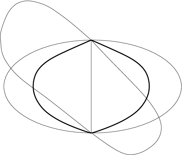
(27)

Specialising (27) for $\alpha=\pi/2$ , and using the fact that $x^{2}-y^{2}-1\leqslant x^{2}+y^{2}-1<0$ , we see that the second component of the above vector vanishes. Thus any point $(x,iy)$ projects onto $(x,0)$ , which means that $P_{\pi/2}$ is contained in $S_{\gamma,P}$ .
We examine now the case where $\alpha\neq\pi/2$ . Pick a point $m$ on $\partial P_{\alpha}$ distinct from $(\pm 1,0)$ . The expression (27) becomes (using $x^{2}+y^{2}=1$ and $\sin{\alpha}>0$ ):

\begin{bmatrix}x\\ ye^{i\alpha}\\ 1\end{bmatrix}-ie^{\alpha}\begin{bmatrix}x\\ ye^{-i\alpha}\\ 1\end{bmatrix}.

(28)

which corresponds after projectivizing and rearranging to the point with coordinates

\left(x,\dfrac{y\cos{\alpha}}{1+\sin\alpha}\right).

As a consequence, we see that a point $m=(x,ye^{i\alpha})\in\partial P_{\alpha}$ with $y>0$ (resp. $y<0$ ) projects onto $P^{+}$ (resp. $P^{-}$ ) if and only if $\alpha\in]0,\pi/2[$ , and that the situation is opposite when $\alpha\in]\pi/2,\pi[$ . This proves the result for connected components of the boundary of $P_{\alpha}$ .

To conclude, let us assume that $\cos{\alpha}>0$ and that there is a point $m=(x,ye^{i\alpha})$ in $P_{\alpha}$ with $y>0$ projecting onto $P^{-}$ . Then, considering the segment $\{(x,te^{i\alpha}),t\in[y,\sqrt{1-y^{2}}]\}$ connecting $m$ to $\partial P_{\alpha}$ , we find a point with coordinates $(x,y^{\prime}e^{\alpha})\in P_{\alpha}$ which projects to a point of $P$ with vanishing $y$ coordinate, that is a point of $\gamma$ . Applying if necessary a loxodromic element in $R_{\gamma}$ (see Proposition 4 and Definition 2), we may assume that the projection is actually the point $(0,0)$ . Since the fiber of $\Pi$ above $(0,0)$ is $i\mathbb{H}^{2}_{\mathbb{R}}$ , this yields $\alpha=\pi/2$ , which is absurd. The case where $\cos{\alpha}<0$ is done in the same way. This proves the result ∎

We give now another characterisation of spinal $\mathbb{R}$ -surfaces. Recall that if $\gamma$ is a geodesic, $R_{\gamma}$ is the 1-parameter subgroup of PU(2,1) associated to $\gamma$ . It contains the loxodromic isometries of real trace greater than 3 preserving $\gamma$ (see Definition 2).

Lemma 5.

Let $Q$ be a real plane, and $\gamma$ be a geodesic of which endpoints we denote by $p$ and $q$ . Assume that the real symmetry about $Q$ satisfies $\sigma_{Q}(p)=q$ . Then the union $\cup_{g\in R_{\gamma}}g\cdot Q$ is a spinal $\mathbb{R}$ -surface. Conversely, any spinal $\mathbb{R}$ -surface may be obtained in this way.

Proof.

We may normalise the situation so that, using the ball model of $\mathbb{H}^{2}_{\mathbb{C}}$ , the points $p$ and $q$ have coordinates $p=(-1,0)$ and $q=(1,0)$ , and $Q$ is the real plane $i\mathbb{H}^{2}_{\mathbb{R}}$ . The 1-parameter subgroup $R_{\gamma}$ preserves the real plane $\mathbb{H}^{2}_{\mathbb{R}}$ and acts transitively on the geodesic connecting $p$ and $q$ . Since $i\mathbb{H}^{2}_{\mathbb{R}}$ is the fibre of the orthogonal projection onto $\mathbb{H}^{2}_{\mathbb{R}}$ above the point $(0,0)$ which belongs to $\gamma$ , we see that $\cup_{g\in R_{\gamma}}g\cdot i\mathbb{H}^{2}_{\mathbb{R}}$ is the spinal $\mathbb{R}$ -surface built on $\gamma$ with respect to $P$ . ∎

As said above, spinal surfaces enjoy two equivalent definitions, either as inverse images of geodesics for the orthogonal projection onto complex lines, or as surfaces equidistant from two given points in $\mathbb{H}^{2}_{\mathbb{C}}$ . We have so far given an analogue of the first definition for spinal $\mathbb{R}$ -surfaces. The next proposition is more in the flavour of the second one: it is possible to see spinal $\mathbb{R}$ -surfaces as natural obects separating two adjacent real ideal triangles, just as spinal surfaces are naturally separating two distinct points. This version of the definition will be of use to understand the geometric meaning of the third part of Theorem 2.

Proposition 15.

Let $\tau=(m_{1},m_{2},m_{3})$ and $\tau^{\prime}=(m_{1},m_{3},m_{4})$ be two ideal real triangles and $\gamma$ be the geodesic connecting $m_{1}$ and $m_{3}$ . Assume that the argument of ${\tt Z}(\tau,\tau^{\prime})$ is not $\pi$ . Then there exists a unique spinal $\mathbb{R}$ -surface $S$ built on the geodesic $\gamma$ having the mirror of $\sigma_{\tau,\tau^{\prime}}$ as one of its leaves.

Recall that $\sigma_{\tau,\tau^{\prime}}$ is the symmetry of the pair $(\tau,\tau^{\prime})$ (see Definition 6).

Proof.

Let $P$ be the mirror of $\sigma_{\tau,\tau^{\prime}}$ . Applying Lemma 5 to the real plane $P$ and the geodesic $\gamma$ , we obtain a spinal $\mathbb{R}$ -surface having the requested property. If there were another spinal $\mathbb{R}$ -surface having the same property, the uniqueness part in Lemma 6 would show that it would have $P$ as a leaf, and contain $\gamma$ . Thus it would be equal to $S$ by Lemma 5. ∎

Definition 18.

Let $\tau$ and $\tau$ be two real ideal triangles sharing an edge and such that the argument of ${\tt Z}(\tau,\tau^{\prime})$ is not $\pi$ . We will call the spinal $\mathbb{R}$ -surface given by Proposition 15 the splitting surface of $\tau$ and $\tau^{\prime}$ and denote it by Spl $(\tau,\tau^{\prime})$ .

Remark 18.

The definition of the splitting surface implies directly that Spl $(\tau_{1},\tau_{2})$ =Spl $(\tau_{2},\tau_{1})$ .

Proposition 16.

Let $\tau$ and $\tau^{\prime}$ be two adjacent ideal triangles such that $\texttt{Z}(\tau,\tau^{\prime})$ has argument different from $\pi$ . Then $\tau$ and $\tau^{\prime}$ belong to opposite connected components of $\mathbb{H}^{2}_{\mathbb{C}}\setminus\mbox{Spl}(\tau,\tau^{\prime})$ .

Proof.

Since two spinal $\mathbb{R}$ -surfaces are isometric, we may normalise the situation in such a way that the common geodesic of $\tau$ and $\tau^{\prime}$ is in ball coordinates $\gamma=\{(x,0),x\in]-1,1[\}$ , the splitting surface of $\tau$ and $\tau^{\prime}$ is $S_{\gamma,\mathbb{H}^{2}_{\mathbb{R}}}$ , and the symmetry $\sigma_{\tau,\tau^{\prime}}$ of the pair $(\tau,\tau^{\prime})$ is the real symmetry about $i\mathbb{H}^{2}_{\mathbb{R}}$ , which is given in coordinates by

(z_{1},z_{2})\longmapsto(-\bar{z}_{1},-\bar{z}_{2}).

We are in the same situation as in the proof of Proposition 14: $\tau$ is contained in one of the real planes $P_{\alpha}$ . Since $\tau^{\prime}$ and $\tau$ are exchanged by $\sigma_{\tau,\tau^{\prime}}$ , $\tau^{\prime}$ is contained in the real plane $\sigma_{\tau,\tau^{\prime}}(P_{\alpha})$ , which is $P_{-\alpha}$ . The result is then a direct application of Proposition 14. ∎

Proposition 17.

The splitting surface associated to a pair of adjacent real ideal triangles is determined by the argument of their ${\tt Z}$ -invariant.

Proof.

Let $\tau$ be a real ideal triangle, and $\gamma$ be one of its edges. Consider $\tau_{1}$ and $\tau_{2}$ two real ideal triangles sharing the edge $\gamma$ with $\tau$ such that ${\tt Z}(\tau,\tau_{j})=x_{j}e^{i\alpha}$ for $j=1,2$ . We have to show that the two spinal $\mathbb{R}$ -surfaces Spl $(\tau,\tau_{1})$ and Spl $(\tau,\tau_{2})$ coincide.

Call $Q_{1}$ and $Q_{2}$ the mirrors of the symmetries of the pairs $(\tau,\tau_{1})$ and $(\tau,\tau_{2})$ . Proposition 7 provides us a unique isometry $g$ belonging to the 1-parameter subgroup $G_{\gamma}$ which maps $Q_{1}$ to $Q_{2}$ . In view of Lemma 5, the result is proved. ∎

5.3 Proof of the third part of theorem 2

We will prove now that a representation $\rho$ associated to a regular bending decoration ${\tt D}$ with anugular part $\theta\in[-\pi/2,\pi/2]$ is discrete and faithful. It is sufficient to prove that for these values of $\theta$ , the action of $\rho(\pi_{1}(\Sigma))$ acts properly discontinuously on some $\rho(\pi_{1}(\Sigma))$ -invariant subset of $\mathbb{H}^{2}_{\mathbb{C}}$ . The following result is the crucial technical point.

Theorem 3.

Let $\tau$ be a real ideal triangle with vertices $(p_{1},p_{2},p_{3})$ . For $i=1,2,3$ , let $\gamma_{i}$ be the geodesic $p_{i+1}p_{i+2}$ (indices taken mod. 3). Let $\tau_{1}$ , $\tau_{2}$ and $\tau_{3}$ be real ideal triangles, such that

•

For $i=1,2,3$ , $\tau$ and $\tau_{i}$ are adjacent, and share the geodesic $\gamma_{i}$ as an edge.
•

There exists $\theta\in[-\pi/2,\pi/2]$ such that $\mbox{arg}\left({\tt Z}(\tau,\tau_{i})\right)=\theta$ for $i=1,2,3$ .

Then the three splitting surfaces $S_{i}={\rm Spl}(\tau,\tau_{i})$ ( $i=1,2,3$ ) enjoy the following properties.

1.

The intersection of $S_{i}$ and $S_{i+1}$ in $\mathbb{H}^{2}_{\mathbb{C}}$ is empty.
2.

The intersection of the closures of $S_{i}$ and $S_{i+1}$ in $\mathbb{H}^{2}_{\mathbb{C}}\cup\partial\mathbb{H}^{2}_{\mathbb{C}}$ is exactly $\{p_{i+2}\}$ .

We postpone the proof of Theorem 3, and first finish the proof of Theorem 2.

Proof of part 3 of Theorem 2.

Consider a given bipartite ideal triangulation $T$ of $\Sigma$ and a regular bending decoration ${\tt D}$ of $T$ with bending angle $\alpha$ . From ${\tt D}$ , we can construct as in the proof of Theorem 1 a family of real ideal triangles in $\mathbb{H}^{2}_{\mathbb{C}}$ , and a $T$ -bent realisation $(\phi,\rho)$ of $\mathcal{F}_{\infty}$ such that any two neighbouring triangles $(\Delta,\Delta^{\prime})$ in $\hat{T}$ are mapped by $\phi$ to two real ideal triangle $(\tau,\tau^{\prime})$ with a common edge and such that $\mbox{arg}(\texttt{Z}(\tau,\tau^{\prime}))=\pm\alpha$ . We associate to each such pair of ideal triangle its splitting surface $Spl(\tau,\tau^{\prime})$ . Proposition 16 implies that $\tau$ and $\tau^{\prime}$ lie in opposite connected components of $\mathbb{H}^{2}_{\mathbb{C}}\setminus Spl(\tau,\tau^{\prime})$ . Now, let $\tau$ be a triangle in the family, and $(\tau_{i})_{i=1,2,3}$ be its three neighbours. Because of the regularity of the bending decoration, we have

\mbox{arg}{\left(\texttt{Z}(\tau,\tau_{1})\right)}=\mbox{arg}{\left(\texttt{Z}(\tau,\tau_{2})\right)}=\mbox{arg}{\left(\texttt{Z}(\tau,\tau_{3})\right)}=\pm\alpha.

(29)

Since $\alpha\in[-\pi/2,\pi/2]$ , we can apply Theorem 3, and conclude that the three splitting surfaces $Spl(\tau,\tau_{i})$ are disjoint. Therefore each of the triangles $\tau$ obtained from the bending decoration belong to a prism $\mathfrak{p}_{\tau}$ , which is the connected component of $\mathbb{H}^{2}_{\mathbb{C}}\setminus\left(Spl(\tau,\tau_{1})\cup Spl(\tau,\tau_{2})\cup Spl(\tau,\tau_{3})\right)$ whose boundary is made of three spinal $\mathbb{R}$ -surfaces. Applying reccursively Proposition 16 shows that any two such prisms are either equal or disjoint. As a consequence, we see that $\rho(\pi_{1}(\Sigma))$ acts on the union of all the prims in such a way that

\rho(\gamma)\cdot\mathfrak{p}_{\tau}=\mathfrak{p}_{\rho(\gamma)(\tau)},\mbox{for any }\gamma\in\pi_{1}(\Sigma).

Therefore the action is discontinuous on $\cup_{\Delta\in\hat{T}}\mathfrak{p}_{\Delta}$ , and $\rho$ is discrete. ∎

We prove now Theorem 3.

Proof of Theorem 3.

$\mbox{(See figure \ref{piccrucial}})$ .

First step: reduction to a normalised case.
By applying if necessary an isometry, we may assume that $\tau$ is the reference real ideal triangle given by $p_{1}=\infty$ , $p_{2}=[-1,0]$ and $p_{3}=[0,0]$ . The isometry $\mathcal{E}$ given in by (18) in Definition 12 cyclically permutes the three latter points, and preserves the invariant Z of pairs of real ideal triangles since it is holomorphic. The bending decoration being regular, the invariants ${\tt Z}(\tau,\tau_{i})$ and ${\tt Z}(\tau,\tau_{j})$ have the same argument. Therefore $\mathcal{E}$ maps $\tau_{i}$ to an ideal $\mathbb{R}$ -triangle $\tau^{\prime}_{i+1}$ (indices taken mod. $3$ ) such that ${\tt Z}(\tau,\tau_{i+1})$ and ${\tt Z}(\tau,\tau^{\prime}_{i+1})$ have the same argument. As a consequence of Proposition 17, it maps the splitting surface $S_{i}$ to $S_{i+1}$ , that is, it permutes the three splitting surfaces cyclically. Hence it is enough to prove that the two surfaces $S_{1}$ and $S_{2}$ satisfy 1 and 2.

Second step : parametrisation of the symmetries about the leaves of $S_{2}$ and $S_{3}$ .
Let us use the following lifts for the $p_{i}$ ’s:

{\bf p}_{1}=\begin{bmatrix}1\\ 0\\ 0\end{bmatrix},{\bf p}_{2}=\begin{bmatrix}-1\\ -\sqrt{2}\\ 1\end{bmatrix}\mbox{ and }{\bf p}_{3}=\begin{bmatrix}0\\ 0\\ 1\end{bmatrix}.

(30)

We first use Lemma 5 to describe the leaves of $S_{2}$ . Let $q_{2}$ be the third point of $\tau_{2}$ . According to Proposition 17, we may assume that $q_{2}$ is any point such that ${\tt Z}(\tau,\tau_{2})$ has the form $xe^{i\theta}$ with $x>0$ . We make the choice $q_{2}=[e^{i\theta},0]$ . The unique symmetry about a real plane swapping $p_{1}$ and $p_{3}$ , and $p_{2}$ and $q_{2}$ is given by $\sigma_{2}(m)={\bf P}\left(M_{2}{\bf m}\right)$ , where $M_{2}$ is the matrix

M_{2}^{\theta}=\begin{bmatrix}0&0&1\\ 0&e^{i\theta}&0\\ 1&0&0\end{bmatrix}.

The 1-parameter subgroup $R_{\gamma_{2}}$ associated to the geodesic connecting $p_{1}$ and $p_{3}$ is parametrised by the matrices

{\bf D}_{r_{2}}=\begin{bmatrix}r_{2}&0&0\\ 0&1&0\\ 0&0&1/r_{2}\end{bmatrix}\mbox{ with }r_{2}>0.

(31)

We obtain thus the general form $M^{\theta}_{2,r_{2}}$ of a lift of the symmetry about a leaf of $S_{1}$ by conjugating a lift of the involution associated to $M_{2}^{\theta}$ by ${\bf D}_{r_{2}}$ . Since $M_{2}^{\theta}$ stands for a antiholomorphic isometry, this yields (see Remark 2)

$\displaystyle M^{\theta}_{2,r_{2}}$	$\displaystyle=$	$\displaystyle{\bf D}_{r_{2}}M_{2}^{\theta}\overline{{\bf D}_{r_{2}}^{-1}}$	(32)
	$\displaystyle=$	$\displaystyle{\bf D}_{r_{2}}M_{2}^{\theta}{\bf D}_{1/r_{2}}\mbox{ (${\bf D}_{1/r_{2}}$ has real coefficients)}$
	$\displaystyle=$	$\displaystyle\begin{bmatrix}0&0&r_{2}^{2}\\ 0&e^{i\theta}&0\\ 1/r_{2}^{2}&0&0\end{bmatrix}.$

The general form $M^{\theta}_{3,r_{3}}$ of a lift of the symmetry about a leaf of $S_{3}$ is obtained by conjugating the matrix $M^{\theta}_{3,r_{3}}$ by the order three elliptic element $\mathcal{E}$ :

$\displaystyle M^{\theta}_{3,r_{3}}$	$\displaystyle=$	$\displaystyle\mathcal{E}{\bf D}_{r_{3}}M_{2}^{\theta}\overline{{\bf D}_{r_{3}}^{-1}}\overline{E^{-1}}$	(33)
	$\displaystyle=$	$\displaystyle\mathcal{E}{\bf D}_{r_{3}}M_{1}^{\theta}{\bf D}_{1/r_{3}}\mathcal{E}^{-1}$
	$\displaystyle=$	$\displaystyle\begin{bmatrix}-r_{3}^{2}&\sqrt{2}\left(e^{i\theta}+r_{3}^{2}\right)&\dfrac{1+2e^{i\theta}r_{3}^{2}+r_{3}^{4}}{r_{3}^{2}}\\ &&\\ \sqrt{2}r_{3}^{2}&e^{i\theta}+2r_{3}^{2}&\sqrt{2}\left(e^{i\theta}+r_{3}^{2}\right)\\ &&\\ r_{3}^{2}&-\sqrt{2}r_{3}^{2}&-r_{3}^{2}\end{bmatrix}.$

Third step: proof of the disjunction
Note first that the closures of $S_{2}$ and $S_{3}$ in $\mathbb{H}^{2}_{\mathbb{C}}\cup\partial\mathbb{H}^{2}_{\mathbb{C}}$ both contain the point $p_{1}$ as a common end of the geodesics $\gamma_{2}$ and $\gamma_{3}$ . Therefore their intersection should at least contain this point. Now, the result will be proved if we show that the closure of any leaf of $S_{2}$ is disjoint from the closure or any leaf of $S_{3}$ . We do this by showing that the product of the symmetries about these leaves is loxodromic as long as $\theta\in[-\pi/2,\pi/2]$ (see Lemma 1). More precisely, we will show that for these values of $\theta$ , the isometry associated to the matrix $M^{\theta}_{2,r_{3}}\overline{M^{\theta}_{3,r_{3}}}$ is loxodromic for any pair $(r_{2},r_{3})\in\mathbb{R}_{>0}^{2}$ . Using the above matrix form, it is seen that the trace of this matrix is

\mbox{\rm tr}M^{\theta}_{2,r_{2}}\overline{M^{\theta}_{3,r_{3}}}=2r_{3}^{2}e^{i\theta}+\frac{2}{r_{2}^{2}}e^{-i\theta}+1+r_{2}^{2}r_{3}^{2}+\frac{1}{r_{2}^{2}r_{3}^{2}}+\frac{r_{3}^{2}}{r_{2}^{2}}.

(34)

This yields

$\displaystyle\mbox{\rm Re}\,\left(\mbox{\rm tr}M^{\theta}_{2,r_{2}}\overline{M^{\theta}_{3,r_{3}}}\right)$	$\displaystyle=$	$\displaystyle 2r_{3}^{2}\cos{\theta}+\frac{2}{r_{2}^{2}}\cos{\theta}+1+r_{2}^{2}r_{3}^{2}+\frac{1}{r_{2}^{2}r_{3}^{2}}+\frac{r_{3}^{2}}{r_{2}^{2}}$	(35)
	$\displaystyle\geqslant$	$\displaystyle 1+r_{2}^{2}r_{3}^{2}+\frac{1}{r_{2}^{2}r_{3}^{2}}\mbox{ while }\cos{\theta}\geqslant 0$
	$\displaystyle\geqslant$	$\displaystyle 3$

This implies that the isometry associated to $M^{\theta}_{2,r_{3}}\overline{M^{\theta}_{3,r_{3}}}$ is loxodromic as long as $\theta\in[-\pi/2,\pi/2]$ and for any pair $(r_{2},r_{3})\in\mathbb{R}_{>0}^{2}$ , as shown by Remark 3. As a consequence of Lemma 1, the corresponding leaves of $S_{2}$ and $S_{3}$ are disjoint. ∎

Remark 19.

In the case of PSL(2, $\mathbb{R}$ ), or more generally in the case of real split Lie groups, it is possible to prove the discreteness of the image of $\rho$ by studying the coordinate changes induced by the flip moves: these moves preserve the positivity of cross-ratios, and this leads to the discreteness of $\rho$ (see for instance [12] pages 87 to 89). Such an approach is not possible here. Notice for instance that if $(a,b,c)$ and $(c,d,a)$ are real ideal triangles sharing an edge, then the two ideal triangles obtained after a flip move, namely $(a,b,d)$ and $(b,c,d)$ are not real in general.

6 Remarks and comments

6.1 The case of real positive decorations : $\mathbb{R}$ -Fuchsian representations.

Let us focus for a moment on the special case where the bending decoration is positive: for all edge $e$ of $T$ , ${\tt D}(e)\in\mathbb{R}>0$ . It this case, all the triangles constructed from ${\tt D}$ are contained in the standard real plane $\mathbb{H}^{2}_{\mathbb{R}}$ . As mentionned in Remark 12, the Z-invariant is in this case the usual cross-ratio in the upper half-plane. We recover this way the classical shear coordinates, and the action of the $\rho(\pi_{1}(\Sigma))$ on the upper half-plane, when $\rho$ is a discrete and faithful representation in PSL(2, $\mathbb{R}$ ). This corresponds to the embedding $\mbox{\rm PSL(2,$\mathbb{R}$)}\sim\mbox{PO(2,1)}$ as the stabilizer of $\mathbb{H}^{2}_{\mathbb{R}}$ . Moreover, when $z\in\mathbb{R}_{>0}$ , the restriction of the real symmetry $\sigma_{z}$ to $\mathbb{H}^{2}_{\mathbb{R}}$ is a half-turn. We recover thus also the explicit combinatorial description of classes of discrete and faithful representations in PSL(2, $\mathbb{R}$ ) given for instance by Fock and Goncharov in [13] by means of elementaries isometries (see section 6.2). Note that the parabolicity criterion for peripheral homotopy classes in [34] or [13] is the same as here (it is expressed in a additive way in [34], where the situation is slightly different, and the coordinates are expressed using logarithms of cross-ratios). In this particular case, if $\tau$ is one of the real ideal triangles constructed from ${\tt D}$ , the prism $\mathfrak{p}_{\tau}$ is the inverse image of $\tau$ by the orthogonal projection onto $\mathbb{H}^{2}_{\mathbb{R}}$ .

6.2 Embeddings of the Teichmüller in the PU(2,1)-representation variety

Let us go back for a moment to the case of representations in PSL(2, $\mathbb{R}$ ), the group of holomorphic isometries of the complex hyperbolic line $\mathbb{H}^{1}_{\mathbb{C}}$ . In this frame, we can define a $\mathbb{H}^{1}_{\mathbb{C}}$ -realisation of the Farey set of a cusped surface $\Sigma$ as a pair $(\phi,\rho)$ , where $\rho:\pi_{1}(\Sigma)\longrightarrow\mbox{\rm PSL(2,$\mathbb{R}$)}$ is a discrete and faithful representation and $\phi$ is a $\rho$ -equivariant mapping from the Farey set to the boundary of the Poincaré disc. Denote by $\mathcal{DF}$ the set of PSL(2, $\mathbb{R}$ )-classes of discrete and faithful representations of $\pi_{1}(\Sigma)$ in PSL(2, $\mathbb{R}$ ), and by $\mathcal{DF}^{+}$ the set of PSL(2, $\mathbb{R}$ )-classes of $\mathbb{H}^{1}_{\mathbb{C}}$ -realizations of $\mathcal{F}_{\infty}(\Sigma)$ .

Let $m$ be a point of $\mathcal{F}_{\infty}(\Sigma)$ , corresponding to a fixed point of a parabolic $c$ , and let $(\phi,\rho)$ be a $\mathbb{H}^{1}_{\mathbb{C}}$ -realisation. The $\rho$ -equivariance of $\phi$ implies that $\phi(m)$ is fixed by $\rho(c)$ . Now, $\rho$ being discrete and faithful, $\rho(c)$ is either parabolic or loxodromic. When $\rho(c)$ is hyperbolic, $\phi(m)$ may be any of the two fixed points of $\rho(c)$ . Consider the projection

	$\displaystyle{\bf p}$	$\displaystyle:$	$\displaystyle\mathcal{DF}^{+}\longrightarrow\mathcal{DF}$		(36)
			$\displaystyle[(\phi,\rho)]\longmapsto[\rho]$		(36)

Let $[[1,n]]$ be the set of integers between $1$ and $n$ . For any subset $I=\{i_{1},\cdots,i_{k}\}$ of $[[1,n]]$ , define

\mathcal{P}_{I}=\left\{[\phi,\rho]\in\mathcal{DF}^{+}|\rho(c_{i})\mbox{ is parabolic }\Leftrightarrow i\in I\right\}.

Then $\mathcal{DF}^{+}$ decomposes as the disjoint union

\mathcal{DF}^{+}=\coprod_{I\subset[[1,n]]}\mathcal{P}_{I},

(37)

and the restriction to $\mathcal{P}_{I}$ of the projection (36) is $2^{n-|I|}$ to 1. In particular, it is $2^{n}$ to 1 when restricted to $\mathcal{P}_{\emptyset}$ , which is the set of realisations associated to totally hyperbolic representations, and it a bijection when restricted to $\mathcal{P}_{[[1,n]]}$ , which corresponds to the Teichmüller space.

Once an ideal triangulation $T$ of $\Sigma$ is fixed, shear coordinates provide a bijection between the set of positive decoration of $T$ (that is, mappings ${\tt d}:e(T)\longrightarrow\mathbb{R}_{>0}$ ), and the set of $\mathcal{DF}^{+}$ . The main tool is the classical cross-ratio, used as a gluing invariant of two ideal triangles in $\mathbb{H}^{1}_{\mathbb{C}}$ . It is also possible to give an explicit representative for a representation associated to a given decoration by use of elementary isometries. This time, the elementary isometries are

I_{x}=\begin{bmatrix}0&\sqrt{x}\\ -1/\sqrt{x}&0\end{bmatrix},

for an edge of type 1 intersecting an edge of $T$ decorated by the positive number $x$ , and

E=\begin{bmatrix}1&1\\ -1&0\end{bmatrix},

for a positively oriented edge of type 2. The mechanic of the construction is the same as what we did in section 4, only simplified by the fact that both types of elementary isometries are holomorphic, thus there is no need of colouring faces of $\hat{T}$ in the classical case. This material is classical and exposed for instance in [13]. Notice that if $c_{j}$ is a peripheral homotopy class around the deleted point $x_{j}$ , the parabolicity of $\rho(c_{j})$ is equivalent to the condition that the associated positive decoration is balanced at $x$ (that is, the product of all positive numbers on edges adjacent to $x$ equals 1). Type-preserving representations, and therefore the Teichmüller space of $\Sigma$ correspond to positive decorations which are balanced at every deleted point of $\Sigma$ . We call such decorations simply balanced.

Fix a bipartite ideal triangulation $T$ . The set of positive decorations of $T$ is $\mathbb{R}_{>0}^{\sharp e(T)}$ . To any real number $\theta$ is associated a mapping

	$\displaystyle\psi_{\theta}$	$\displaystyle:$	$\displaystyle\mathbb{R}_{>0}^{\sharp e(T)}\longrightarrow\mathcal{BD}_{T}$		(38)
			$\displaystyle{\tt d}\longmapsto{\tt D}={\tt d}e^{i\theta}.$		(38)

This mapping induces a mapping from $\mathcal{DF}^{+}$ to $\mathcal{BR}_{T}$ , which maps the realisation associated to ${\tt d}$ to the $T$ -bent realisation associated to the regular bending decoration ${\tt d}e^{i\theta}$ . Restricting this induced mapping to those $\mathbb{H}^{1}_{\mathbb{C}}$ -realisation corresponding to balanced positive decorations, we can rephrase Theorem 2 as follows.

Theorem 4.

Let $\theta\in[-\pi/2,\pi/2]$ be a real number and $T$ be a bipartite ideal triangulation of $\Sigma$ . The mapping $\psi_{\theta}$ defined in (38) induces a pair of embeddings of $\mathcal{DF}(\Sigma)$ of $\Sigma$ in Hom( $\pi_{1}$ , PU(2,1))/PU(2,1) of which images contain only classes of discrete and faithful representations.

Proof.

Restricting the mapping ${\tt d}\longmapsto{\tt d}e^{i\theta}$ to balanced decorations of $T$ produces discrete, faithful and type-preserving representations of $\pi_{1}(\Sigma)$ with images contained in PU(2,1) since $T$ is bipartite. Once a coloring of the faces of $\hat{T}$ is fixed, we obtain two injective applications by mapping the point in $\mathcal{T}(\Sigma)$ associated to ${\tt d}$ to the class of representations associated to ${\tt d}e^{i\theta}$ corresponding either to white triangles or to black triangles. These two embeddings are identified by the complex conjugation in $\mathbb{H}^{2}_{\mathbb{C}}$ , and correspond in fact to a single embedding in Hom( $\pi_{1}$ ,PU(2,1))/Isom( $\mathbb{H}^{2}_{\mathbb{C}}$ ). ∎

Note that Theorem 2 states as well that the parabolicity of images of peripheral loops is preserved by $\psi_{\theta}$ , and thus the image of $\psi_{\theta}$ admits a similar decomposition as (37).

6.3 Link with previously known families of examples.

In this section, we draw the connection between $T$ -bent realizations and families of examples described in the previous works [9, 24, 42].

The 1-punctured torus.

In this case $T$ consists of two triangles, as indicated on figure 10. We will use the vertex $v$ marked on the figure as basepoint. There are two faces, of which colour is indicated by ${\tt w}$ and ${\tt b}$ on figure 10, and three edges, labelled by $e_{1}$ , $e_{2}$ and $e_{3}$ on figure 10. In the case of a regular bending decorations,the decoration is given three positive real numbers $x_{1}$ , $x_{2}$ and $x_{3}$ and $\theta\in[0,2\pi[$ such that the edge $e_{i}$ is decorated by $x_{i},\theta$ . Following the results of section 4.3, we see that the identifications between opposite faces of the square correspond to the following holomorphic isometries of $\mathbb{H}^{2}_{\mathbb{C}}$ . Call $A$ and $B$ the isometries associated respectively to the horizontal and vertical identifications of the opposite sides of the square. Following section 4.3, these isometries are given by

\left\{\begin{matrix}A&=&\mathcal{E}\circ\sigma_{x_{2},\theta}\circ\mathcal{E}^{-1}\circ\sigma_{x_{2},\theta}\\ \\ B&=&\sigma_{x_{2},\theta}\circ\mathcal{E}^{-1}\circ\sigma_{x_{3},\theta}\circ\mathcal{E}.\end{matrix}\right.

(39)

As a consequence, we see that the group $\langle A,B\rangle$ has index two in the group generated by the three real symmetries $I_{1}=\mathcal{E}\circ\sigma_{x_{1},\theta}\circ\mathcal{E}^{-1}$ , $I_{2}=\sigma_{x_{2},\theta}$ and $I_{3}=\mathcal{E}^{-1}\circ\sigma_{x_{3},\theta}\circ\mathcal{E}$ . The group $\langle I_{1},I_{2},I_{3}\rangle$ is an example of a so-called Lagrangian triangle group. This example of bending has been exposed with a different point of view in [42] (see also[41]).

In [42], the discreteness result is stated with an angle $\alpha\in[-\pi/4,\pi/4]$ . This angle $\alpha$ is actually half the bending parameter $\theta$ we use here. It may be interpreted as an angle between a real ideal triangle $\Delta$ and the splitting surface Spl( $\Delta,\Delta^{\prime}$ ), where $\Delta^{\prime}$ is adjacent to $\Delta$ . From this point of view, Spl( $\Delta$ , $\Delta^{\prime}$ ) is bisecting the pair $(\Delta,\Delta^{\prime})$ .

The Toledo invariant and the examples of Gusevskii and Parker

The Toledo invariant is a conjugacy invariant defined for representations of fundamental groups of closed surfaces, and for type-preserving representations of cusped surfaces. We refer the reader to [40] and [27, 24] for its definition and main properties. Let us just recall that if $\rho$ is such a representation, then

•

if $\Sigma$ has punctures, then ${\bf tol}(\rho)$ is a real number in the interval $[-\chi,\chi]$ , where $\chi$ is the Euler characteristic of $\Sigma$ ,
•

if not, then ${{\bf tol}}(\rho)$ belongs to $2/3\mathbb{Z}\cap[\chi,-\chi]$ .

Let $(\phi,\rho)$ be a $T$ -bent realization of $\mathcal{F}_{\infty}$ , where $T$ is a bipartite triangulation, and $\Omega$ be a fundamental domain for the action of $\pi_{1}(\Sigma)$ on $\tilde{\Sigma}$ . We might see $\Omega$ as a family of triangles $(\Delta_{1},\cdots,\Delta_{m})$ . Then it follows from [24, 40] that the Toledo invariant ${\bf tol}(\rho)$ equals twice the sum of the Cartan invariants of the ideal triangles $\phi(\Delta_{i})$ . In our particular case, all the triangles are real. We obtain therefore directly the

Proposition 18.

Let $(\phi,\rho)$ be a $T$ -bent realization of $\mathcal{F}_{\infty}$ , with $\rho$ type-preserving. The Toledo invariant of $\rho$ is equal to zero.

In [24], Gusevskii and Parker have described for each genus $g$ and number of punctures $n$ a 1-parameter family $(\rho_{t})_{t\in[-\chi,\chi]}$ of non PU(2,1)-equivalent discrete, faithful and type-preserving representations of a Riemann surface of genus $g$ with $n$ punctures having the property that the Toledo invariant of $\rho_{t}$ equals $t$ . This shows that all the possible values of the Toledo invariant for non-compact surfaces are realised by discrete and faithful representation. To prove this result, Gusevskii and Parker start from discrete and faithful representations of the modular group in PU(2,1) and pass to a finite index subgroup using Millington’s theorem (see [24]). In their construction, they show that $\rho_{0}$ preserves a real plane (this is a so-called $\mathbb{R}$ -Fuchsian representation). Therefore $\rho_{0}$ is the unique intersection between Gusevskii and Parker’s family of representations and our one.

The 3-punctured sphere and the examples of Falbel and Koseleff.

This time we are using the bipartite triangulation of the 3-punctured sphere showed on figure 11. The representation of the fundamental group associated to the decoration given by $\delta(e_{i})=x_{i}$ and $\alpha(e_{i})=\theta_{i}$ is given by

\left\{\begin{matrix}A&=&\mathcal{E}^{-1}\circ\sigma_{x_{1},\theta_{1}}\circ\mathcal{E}^{-1}\circ\sigma_{x_{2},\theta_{2}}\\ \\ B&=&\sigma_{x_{2},\theta_{2}}\circ\mathcal{E}^{-1}\circ\sigma_{x_{3},\theta_{3}}\circ\mathcal{E}^{-1}.\\ \\ C&=&\mathcal{E}\circ\sigma_{x_{3},\theta_{3}}\circ\mathcal{E}^{-1}\circ\sigma_{x_{1},\theta_{1}}\circ\mathcal{E},\end{matrix}\right.

(40)

It is easily checked that $ABC=1$ . Using the matrices given in section 4.3, we see that the representation is type preserving if and only if $x_{1}=x_{2}=x_{3}=1$ and none of the $\theta_{i}$ ’s is equal to $\pi$ . When $\theta_{1}=\theta_{2}=\theta_{3}\in[-\pi/2,\pi/2]$ , this provides through theorem 2 a 1-parameter family of discrete, faithful and type-preserving representations of the fundamental group of the 3-punctured sphere.

Moreover, it is possible to prove that in the case where $\delta(e_{i})=1$ and $\alpha(e_{i})=\theta$ for all $i$ , then there exists three real symmetries $s_{1}$ , $s_{2}$ and $s_{3}$ such that $A=s_{1}s_{2}$ and $B=s_{2}s_{3}$ . Call $Q_{i}$ the mirror of $s_{i}$ . Since $A$ and $B$ are parabolic, the mirrors of the $s_{i}$ ’s are mutually asymptotic, that is $Q_{i}\cap Q_{i+1}$ consists of exactly one point in $\partial\mathbb{H}^{2}_{\mathbb{C}}$ . Therefore these groups belong to the family of groups studied by Falbel and Koseleff in [9]. Note moreover that the discreteness of these groups was not proved in [9], where the focus is on deformations of groups preserving a complex line.

References

[1] S. Anan’in, C.H. Grossi, and N. Gusevskii. Complex Hyperbolic Structures on Disc Bundles over Surfaces I. General Settings. A Series of Examples. arXiv:math/0511741, 2005.
[2] S. Anan’in, C.H. Grossi, and N. Gusevskii. Complex Hyperbolic Structures on Disc Bundles over Surfaces II. Example of a Trivial Bundle. arXiv:math/0512406, 2005.
[3] B. Apanasov. Bending deformations of complex hyperbolic surfaces. J. reine angew. Math, 492:75–91, 1997, MR1488065, Zbl 0891.53055.
[4] F. Bonahon. Shearing hyperbolic surfaces, bending pleated surfaces and Thurston’s symplectic form. Ann. Fac. Sci. Toulouse Math., 5, 1996. MR1413855, Zbl 0880.57005.
[5] M. Burger, A. Iozzi, F. Labourie, and A. Wienhard. Maximal representations of surface groups: symplectic Anosov structures. Pure Appl. Math. Q.1, 2005. MR2201327, Zbl 1157.53025
[6] M. Burger, A. Iozzi, and A. Wienhard. Surface group representations with maximal Toledo invariant. Ann. of Math. (2) 172 (2010), no. 1, 517–566. MR2680425, Zbl pre05779363
[7] S. Chen and L. Greenberg. Hyperbolic spaces. Contributions to analysis (a collection of papers dedicated to Lipman Bers), pp. 49–87. Academic Press, New York, 1974. MR0377765,Zbl 0295.53023 .
[8] E. Falbel. Spherical CR structures on the complement of the figure eight knot with discrete holonomy. J. Differential Geom. 79 (2008), no. 1, 69–110. MR2401419, Zbl 1148.57025.
[9] E. Falbel and P.V. Koseleff. Flexibility of ideal triangle groups in complex hyperbolic geometry. Topology 39 (2000), no. 6, 1209–1223. MR1783854, Zbl 0977.32018.
[10] E. Falbel and P.V. Koseleff. Rigidity and flexibility of triangle groups in complex hyperbolic geometry. Topology 41 (2002), no. 4, 767–786. MR1905838, Zbl 1005.32018.
[11] E. Falbel and V. Zocca. A Poincaré polyhedron theorem for complex hyperbolic geometry. J. Reine Angew. Math. 516 (1999), 133–158. MR1724618, Zbl 0944.53042
[12] V. Fock and A.B. Goncharov. Moduli spaces of local systems and higher Teichmüller theory. Publ. Math. Inst. Hautes Études Sci. No. 103 (2006), 1–211. MR2233852,Zbl 1099.14025.
[13] V. Fock and A.B. Goncharov. Dual Teichmüller and lamination spaces. Handbook of Teichmüller theory. Vol. I, 647–684, IRMA Lect. Math. Theor. Phys., 11, Eur. Math. Soc., Zürich, 2007. MR2349682, Zbl 1162.32009.
[14] V. Fock and A.B. Goncharov. Moduli spaces of convex projective structures on surfaces. Moduli spaces of convex projective structures on surfaces. Adv. Math. 208 (2007), no. 1, 249–273. MR2304317, Zbl1111.32013
[15] M. Gaye. Sous-groupes discrets de PU(2,1) engendrés par $n$ réflexions complexes et déformation. Geom. Dedicata 137 (2008), 27–61. MR2449145, Zbl pre05373523.
[16] W. Goldman. Representations of fundamental groups of surfaces. Geometry and topology (College Park, Md., 1983/84), 95–117, Lecture Notes in Math., 1167, Springer, Berlin, 1985. MR0827264, Zbl 0575.57027.
[17] W. Goldman. Topological components of spaces of representations. Invent. Math. 93 (1988), no. 3, 557–607. MR0952283, Zbl 0655.57019
[18] W. Goldman. Complex Hyperbolic Geometry. Oxford Mathematical Monographs. Oxford Science Publications. The Clarendon Press, Oxford University Press, New York, 1999. xx+316 pp. ISBN: 0-19-853793-X. MR1695450, Zbl 0939.32024.
[19] W. Goldman, M. Kapovich, and B. Leeb. Complex hyperbolic manifolds homotopy equivalent to a Riemann surface. Comm. Anal. Geom. 9 (2001), no. 1, 61–95. MR1807952, Zbl 0982.32024
[20] W. Goldman and J. Millson. Local rigidity of discrete groups acting on complex hyperbolic space. Invent. Math. 88 (1987), no. 3, 495–520. MR0884798, Zbl 0627.22012.
[21] W. Goldman and J. Parker. Complex hyperbolic ideal triangle groups. J. Reine Angew. Math. 425 (1992), 71–86. MR1151314, Zbl 0739.53055
[22] O. Guichard. Groupes plongés quasi isométriquement dans un groupe de Lie. Math. Ann. 330 (2004), no. 2, 331–351. MR2089430,Zbl 1061.22014 .
[23] N. Gusevskii and J.R. Parker. Representations of free Fuchsian groups in complex hyperbolic space. Topology 39 (2000), no. 1, 33–60. MR1710991, Zbl 0977.32017.
[24] N. Gusevskii and J.R. Parker. Complex Hyperbolic Quasi-Fuchsian groups and Toledo’s Invariant. Geom. Dedicata 97 (2003), 151–185. MR2003696, Zbl 1042.57023.
[25] N.J. Hitchin. Lie groups and Teichmüller space. Topology 31 (1992), no. 3, 449–473. MR1174252, Zbl 0769.32008.
[26] A. Koranyi and H.M. Reimann. The complex cross-ratio on the Heisenberg group. L’Enseign. Math., (2) 33 (1987), no. 3-4, 291–300. MR0925991, Zbl 0638.22005.
[27] V. Koziarz and J. Maubon. Harmonic maps and representations of non-uniform lattices of PU( $m$ ,1). Ann. Inst. Fourier, 58 (2008), no. 2, 507–558. MR2410381,Zbl 1147.22009.
[28] V. Koziarz and J. Maubon. Representations of complex hyperbolic lattices into rank 2 classical Lie groups of Hermitian type. Geom. Dedicata, 137 (2008), 85–111. MR2449147, Zbl 1159.22006
[29] F. Labourie. Anosov flows, surface groups and curves in projective space. Invent. Math., 165 (2006), no. 1, 51–114. MR2221137, Zbl 1103.32007.
[30] J Marché and P. Will. Configurations of flags and representations of surface groups in complex hyperbolic geometry. Preprint. http://www-fourier.ujf-grenoble.fr/ $\sim$ will/, 2008.
[31] G. D. Mostow. On a remarkable class of polyhedra in complex hyperbolic space. Pac. J. Math., 86 (1980), no. 1, 171–276. MR0586876, Zbl 0456.22012
[32] J. Parker and I. Platis. Open sets of maximal dimension in complex hyperbolic quasi-fuchsian space. J. Diff. Geom, 73 (2006), no. 2, 319–350. MR2226956, Zbl 1100.30037
[33] J. Parker and I. Platis. Complex hyperbolic quasi-Fuchsian groups. Geometry of Riemann surfaces, 309–355, London Math. Soc. Lecture Note Ser., 368, Cambridge Univ. Press, Cambridge, 2010. MR2665016, Zbl pre05722593
[34] R. Penner. The decorated Teichmüller space of punctured surfaces. Comm. Math. Phys., 113 (1987), no. 2, 299–339. MR0919235, Zbl 0642.32012.
[35] G. Platis. Quakebend deformations in complex hyperbolic quasi-Fuchsian space. Geom. Topol., 12 (2008), no. 1, 431–459. MR2390350, Zbl 1153.30038.
[36] R. E. Schwartz. Degenerating the complex hyperbolic ideal triangle groups. Acta Math., 186 (2001), no. 1, 105–154. MR1828374,Zbl 0998.53050.
[37] R. E. Schwartz. Complex hyperbolic triangle groups. Proceedings of the International Congress of Mathematicians, Vol. II (Beijing, 2002), 339–349, Higher Ed. Press, Beijing, 2002. MR1957045, Zbl 1022.53034
[38] R. E. Schwartz. A better proof of the Goldman-Parker conjecture. , Geom. Topol. 9 (2005), 1539–1601 (electronic). MR2175152, Zbl 1098.20034
[39] W. Thurston. Minimal stretch maps between hyperbolic surfaces. preprint math.GT/9801039, 1986.
[40] D. Toledo. Representations of surface groups in complex hyperbolic space. J. Differ. Geom.,29 (1989), no. 1, 125–133. MR0978081,Zbl 0676.57012
[41] P. Will. Groupes triangulaires lagrangiens en géométrie hyperbolique complexe. Actes du Séminaire de Théorie Spectrale et Géométrie. Vol. 25. Année 2006–2007, 189–209, Sémin. Théor. Spectr. Géom., 25, Univ. Grenoble I, Saint-Martin-d’Hères, 2008. MR2478817, Zbl 1159.32007.
[42] P. Will. The punctured torus and Lagrangian triangle groups in PU(2,1). J. reine angew. Math.,602 (2007), 95–121. MR2300453, Zbl 1159.32007.
[43] P. Will. Traces, Cross-ratios and 2-Generator Subgroups of PU(2,1). Canad. J. Math., 61 (2009), no. 6, 1407–1436. MR2588430, Zbl 1185.14038.
[44] E.Z. Xia. The moduli of flat PU(2,1)-structures on Riemann surfaces. Pacific. J. Math., 195 (2000), no. 1, 231–256. MR1781622 , Zbl 1014.32010.

Bending Fuchsian representations of fundamental groups of cusped surfaces in PU(2,1).

Abstract

1 Introduction

Theorem 1 (Bending Theorem).

Theorem 2 (Discreteness Theorem).

Acknowledgements

2 The complex hyperbolic 2-space

2.1 ℍℂ2\mathbb{H}^{2}_{\mathbb{C}} and its isometries

Definition 1.

Proposition 1.

Horospherical coordinates

The ball model of ℍℂ2\mathbb{H}^{2}_{\mathbb{C}}

2.2 Totally geodesic subspaces

The complex lines.

The real planes.

Remark 1.

Computing with real symmetries

Proposition 2.

Proof.

Remark 2.

Lemma 1.

2.3 Classification of isometries.

Proposition 3.

Proof.

Remark 3.

Remark 4.

Loxodromic isometries

Proposition 4.

Proof.

Definition 2.

Remark 5.

Parabolic isometries.

3 Real ideal triangles.

3.1 Ideal triangles

Definition 3.

Proposition 5.

Definition 4.

Remark 6.

3.2 The invariant of a pair of adjacent ideal real triangles.

Lemma 2.

Proof.

Remark 7.

Definition 5.

Remark 8.

Remark 9.

Lemma 3.

Proof.

Proposition 6.

Proof.

Definition 6.

Remark 10.

Remark 11.

Remark 12.

Proposition 7.

Proof.

Remark 13.

4 The bending theorem

4.1 Notation, Definitions

Definition 7.

Definition 8.

Definition 9.

Definition 10.

Definition 11.

Definition 12.

4.2 Bent ℍℂ2\mathbb{H}^{2}_{\mathbb{C}}-realizations : proof of Theorem 1.

Proof of Theorem 1.

4.3 Explicit computation of the representations

Definition 13.

Proposition 8.

Proof.

Proposition 9.

Proof.

4.4 When is the representation in PU(2,1)?

4.4.1 Representations in PU(2,1) and bipartite triangulations

Definition 14.

Remark 14.

Remark 15.

Proposition 10.

Proof.

4.4.2 Existence of bipartite triangulations

2.1 $\mathbb{H}^{2}_{\mathbb{C}}$ and its isometries

The ball model of $\mathbb{H}^{2}_{\mathbb{C}}$

4.2 Bent $\mathbb{H}^{2}_{\mathbb{C}}$ -realizations : proof of Theorem 1.

5.2 Spinal $\mathbb{R}$ -surfaces.

6.1 The case of real positive decorations : $\mathbb{R}$ -Fuchsian representations.