Universality of high-energy absorption cross sections for black holes

During the last 40 years, the study of absorption of waves and particles by black holes and by analogous higher-dimensional objects has received considerable attention, because this topic is directly relevant to numerous fundamental aspects of classical and quantum black hole physics which could permit us to progress in our understanding of spacetime properties. This line of research started around the 1970s (see Refs. [1, 2, 3, 4, 5, 6, 7, 8, 9, 10] for important pioneering works) motivated by absorption of gravitational waves, the superradiance phenomenon, and the Hawking effect. In 1997, a crucial result was obtained by Das, Gibbons and Mathur [11] in connection with string theory: At low energies, i.e., when the wavelength of the particle is much greater than the radius of the black hole horizon, the absorption cross section for a minimally coupled scalar field propagating into a static and spherically symmetric black hole of arbitrary dimension presents a universal behavior, in that it reduces to the area of the black hole horizon. With the extension of this result to the four-dimensional Kerr-Newman black hole by Maldacena and Strominger [12], there has been in the last decade an explosion of the literature concerning this particular theme, with generalizations for all kinds of fields as well as for various extensions of general relativity (see, e.g., Refs. [13, 14, 15, 16, 17, 18, 19, 20, 21, 22, 23, 24, 25], and references therein among hundreds of articles on the subject), some of these works being done with in mind the possibility suggested by brane-world theories that the LHC could behave like a black hole factory (but there are already significant experimental constraints [26]).

At high energies, it is well known that, in general, the absorption cross section of a black hole oscillates around a limiting constant value (see, e.g., Refs. [10, 16, 17, 18, 19, 20, 21, 24, 25]). The existence of this limiting value has been understood a long time ago [27, 28, 29] in terms of geodesics, and it has also been analyzed for wave theories [2, 5, 10]: For a black hole endowed with a photon sphere, the limiting value is exactly the geometrical cross section of this photon sphere, i.e., the so-called capture cross section of the black hole. [Here, it is important to recall that (i) a photon sphere is a hypersurface on which the massless particles can orbit the black hole on unstable circular null geodesics, (ii) its location corresponds to the local maximum of the classical effective potential seen by these massless particles, (iii) a null geodesic arriving from infinity with the critical impact parameter $b_{c}$ approaches the photon sphere asymptotically by spiralling around it, and (iv) the geometrical cross section of the photon sphere is directly related to this critical impact parameter.] As a consequence, at high energies, the limiting value of the absorption cross sections for black holes presents a universal character, but, of course, this does not suffice to conclude on the universality of the high-energy absorption cross sections themselves, because the fluctuations around the limiting value have not yet been explained in terms of black hole properties.

In fact, it is easy to understand why such a universality result currently exists at low frequencies and has not yet an equivalent at high frequencies. In the low-energy regime, the $\ell=0$ partial wave contribution dominates the absorption cross section (it is the only non-vanishing contribution) and it is sufficient to solve only one partial wave equation, in this case, to obtain the universality result. By contrast, at higher energies, we need to sum over the full range of partial waves in order to understand the fluctuations of the absorption cross sections. So it is not possible to provide immediately a clear physical interpretation of this feature. But in this paper, by making use of the Regge pole technique (or, in other words, of the complex angular momentum machinery), we shall realize a resummation of the absorption cross section and then extract the physical information encoded in the sum over all the partial wave contributions. This shall permit us to emphasize the universal character of the fluctuations at high energies, i.e., to show that the existence of these fluctuations is a generic feature of black holes endowed with a photon sphere, which can be described in terms of the area of the geometrical cross section and the properties of the waves trapped near the photon sphere. (Here, it is important to recall that the Regge poles describe the “surface” or Regge waves trapped near the photon sphere and that, from their real and imaginary parts, we obtain, respectively, the nonlinear dispersion relation of these waves and their damping [30, 31, 32].)

We shall first consider the simple and illuminating example of a massless scalar field in the Schwarzschild black hole geometry (Secs. II and III) and then generalize our analysis to a wide class of static and spherically symmetric black holes of arbitrary dimension, which includes various spacetimes of physical interest such as Schwarzschild-Tangherlini and Reissner-Nordström black holes or the canonical acoustic black hole (Sec. IV). We shall finally conclude this paper by a short comment concerning the consequences of our analysis for Hawking radiation, because absorption and emission phenomena are intimately linked through the greybody factors of black holes. Throughout this paper, we shall use units such that $\hbar=c=G=k_{B}=1$ and we shall assume a harmonic time dependence $\exp(-i\omega t)$ for the massless scalar field.

The exterior of the Schwarzschild black hole of mass $M$ can be defined as the manifold ${\cal M}=\hbox{$]-\infty,+\infty[_{t}$}\times]2M,+\infty[_{r}\times S^{2}$ with metric $ds^{2}=-(1-2M/r)dt^{2}+(1-2M/r)^{-1}dr^{2}+d\sigma_{2}^{2}.$ Here $d\sigma_{2}^{2}$ denotes the metric on the unit $2$-sphere $S^{2}$. We recall that this black hole has a photon sphere located at $r=3M$ and that the corresponding critical impact parameter is given by $b_{c}=3\sqrt{3}M$. As a consequence, the geometrical cross section of this black hole is $\sigma_{\mathrm{geo}}=\pi b_{c}^{2}=27\pi M^{2}$ (see, e.g., Chap. 25 of Ref. [29]).

A massless scalar field $\Phi$ propagating on this gravitational background satisfies the wave equation $\Box\Phi=0$, which reduces, after separation of variables and the introduction of the radial partial wave functions $\phi_{\omega\,\ell}(r)$ with $\omega>0$ and $\ell=0,1,2,\dots$, to the Regge-Wheeler equation

In Eq. (1), $r_{\ast}$ is the so-called tortoise coordinate defined from the radial Schwarzschild coordinate $r$ by $dr/dr_{\ast}=(1-2M/r)$, while $V_{\ell}(r_{\ast})$ denotes the Regge-Wheeler potential given by

We recall that $V_{\ell}(r)$ behaves as a potential barrier with a maximum located near the photon sphere radius, i.e., near $r=3M$. For this field and this four-dimensional black hole, the absorption cross section is given by (see e.g. Refs. [2, 5, 10, 33])

where the coefficient $\Gamma_{\ell}(\omega)$ is the absorption probability for a particle with energy $\omega$ and angular momentum $\ell$. It should be also noted that $\Gamma_{\ell}(\omega)$ plays the role of a greybody factor when we consider the emission of particles by the black hole (see also our remarks in the conclusion). When we only consider the absorption phenomenon, we can define $\Gamma_{\ell}(\omega)$ from the solutions $\phi_{\omega\ell}(r)$ of (1) satisfying the boundary conditions

Here $T_{\ell}(\omega)$ and $R_{\ell}(\omega)$ are the transmission and reflection coefficients for absorption by the Schwarzschild black hole, and we have more particularly

In order to extract the information encoded into the sum over all the partial wave contributions (3), we first transform the angular momentum $\ell$ into a complex number $\lambda=\ell+1/2$ and we construct the analytic extension $\Gamma_{\lambda-1/2}(\omega)$ of the greybody factor $\Gamma_{\ell}(\omega)$. It should be noted that there is no unique way to achieve this construction. Such a problem is well-known by practitioners of complex angular momentum techniques (see, e.g., Chap. 13 of Ref. [34]), and we recall that, in general, a suitable interpolation is provided by the simplest extension and is ultimately justified by the results it provides. In our case, we have adopted the following prescription:

where $T_{\lambda-1/2}(\omega)$ is the transmission coefficient for the problem defined by (1), (2) and (4) with $\ell\to\lambda-1/2$ and where ${\overline{T_{{\overline{\lambda}}-1/2}(\omega)}}$ is the transmission coefficient for the same problem but with $\phi_{\ell}(\omega)\to{\overline{{\phi}_{\ell}(\omega)}}$ and $\ell\to{\overline{\lambda}}-\frac{1}{2}$ (here the bar denotes complex conjugation). This prescription allows us to work with the same Regge-Wheeler equation in both cases and gives a consistent analytic extension because $\Gamma_{\lambda-1/2}$ is then clearly a function of $\lambda$ but not $\overline{\lambda}$. On the contrary, note that $|T_{\ell}(\omega)|^{2}$ could not be extended as $T_{\lambda-1/2}(\omega){\overline{T_{\lambda-1/2}(\omega)}}$, because it would be real on all the complex plane and thereby non-analytic since it is not constant. Our prescription will also be justified by another argument below Eq. (21).

It is now interesting to emphasize some important and useful properties of the function $\Gamma_{\lambda-1/2}(\omega)$:

(i) $\Gamma_{\lambda-1/2}(\omega)$ is an even function of $\lambda$. Indeed, $\phi_{\lambda-1/2}(\omega)$ and $\phi_{-\lambda-1/2}(\omega)$ are both solutions of the same Regge-Wheeler problem (1)-(2) and satisfy the same boundary conditions (4). As a consequence, $T_{\lambda-1/2}(\omega)$ and $T_{-\lambda-1/2}(\omega)$ can only differ by a phase factor. This phase factor is necessarily of the type $\exp[i\theta(\lambda)]$, where $\theta(\lambda)$ is a real function. From the prescription (6), we then immediately obtain $\Gamma_{-\lambda-1/2}(\omega)=\Gamma_{\lambda-1/2}(\omega)$.

(ii) The singularities (simple poles) of $\Gamma_{\lambda-1/2}(\omega)$ are symmetrically distributed with respect to the real $\lambda$ axis [as well as symmetrically distributed with respect to the origin $O$ of the complex $\lambda$ plane due to property (i)]: Those associated with $T_{\lambda-1/2}(\omega)$ lie in the first (and in the third) quadrant of the complex $\lambda$ plane and are also the Regge poles $\lambda_{n}(\omega)$, with $n\in\mathbb{N}^{*}$ (where $\mathbb{N}^{*}\equiv\mathbb{N}\setminus\{{0\}}$), of the $S$ matrix of the Schwarzschild black hole (see Refs. [35, 30, 36, 31], and more particularly Fig. 1 of Ref. [31]). Their complex conjugates ${\overline{\lambda_{n}(\omega)}}$ are associated with ${\overline{T_{{\overline{\lambda}}-1/2}(\omega)}}$ and they lie in the fourth (and in the second) quadrant of the complex $\lambda$ plane.

(iii) The residues of $\Gamma_{\lambda-1/2}(\omega)$ at the poles $\lambda_{n}(\omega)$ and ${\overline{\lambda_{n}(\omega)}}$ are complex conjugates of each other and we have in particular

By means of the usual “half-range” Poisson sum formula

we can rewrite the sum (3) as

The integrals in the second term of (9) can be evaluated by using Cauchy’s theorem. To do so, we close the path along the positive real axis with a quarter circle at infinity in the first quadrant of the complex angular momentum plane and a path along the positive imaginary axis going from $+i\infty$ to $0$. The integrals in the third term of (9) can be evaluated similarly but now by closing the path along the positive real axis in the fourth quadrant of the complex angular momentum plane. By noting that all the contributions of the contours at infinity vanish and by taking into account the singularities of the integrands lying in the first and fourth quadrants of the complex $\lambda$ plane, i.e., the poles of the greybody factor $\Gamma_{\lambda-1/2}(\omega)$, we obtain

In Eq. (10), the real part symbol appears because the singularities of $\Gamma_{\lambda-1/2}(\omega)$ lie symmetrically distributed with respect to the real $\lambda$ axis [see properties (ii) and (iii) mentioned in the previous paragraph].

It should be noted that we can simplify (10) by using the relations (for $a\in{\mathbb{R}}$)

as well as the parity of $\Gamma_{\lambda-1/2}(\omega)$. We then obtain

It is important to note that (12) [or equivalently (10)] is an exact expression for the total absorption cross section of the Schwarzschild black hole. Indeed, until now, we have not made any approximation. We have just expressed (3) in a different way. It is also worth pointing out, for the mathematically inclined reader, that (10) and (12) are reminiscent of trace formulas considered in semiclassical analysis and in analytic number theory.

The residue series over the Regge poles of the greybody factor matrix appearing in (12), and given by

provides the oscillating part of the total absorption cross section. From the first and third terms of (12), we can extract the geometrical cross section of the black hole $\sigma_{\mathrm{geo}}=27\pi M^{2}$ (the constant limit of the absorption cross section, which therefore does not play any role in the fluctuations), together with a negligible $\mathcal{O}(1/\omega^{2})$ contribution at high frequencies. Indeed, on the positive real $\lambda$ axis, we can consider that the greybody factor (the absorption probability) is roughly given by

where $\Theta$ is the Heaviside step function, because we know that partial waves characterized by an energy $\omega$ and an angular momentum $\ell$ are totally reflected if $\ell+1/2\gg 3\sqrt{3}M\omega$ and totally absorbed if $\ell+1/2\ll 3\sqrt{3}M\omega$. Then, by inserting (14) into the first term of (12) we obtain exactly the geometrical cross section of the black hole. Of course, it is possible to consider more elaborate models for the greybody factor. For example [see Eq. (19) below], we could assume that, for $\lambda\in[0,+\infty[$,

This expression reduces to (14) for low and high frequencies and it moreover provides an accurate description of the transition between these two regimes, i.e., for $\lambda\approx 3\sqrt{3}M\omega$. By inserting (15) into the first term of (12) we obtain again the geometrical cross section of the black hole but, now, with in addition a correction given by $(\pi/6)/\omega^{2}$. This kind of result seems to be very robust, i.e., independent of any realist model for the greybody factor, and we shall consider that we have always for the first term of (12)

Let us also consider the third term of (12). $\Gamma_{\lambda-1/2}(\omega)$ is bounded on the positive imaginary $\lambda$ axis (it has no poles on this axis, is equal to 1 for $\lambda=0$ and vanishes at $+i\infty$). In fact, we have checked numerically [but a mathematical proof involving the fact that $1/\Gamma_{\lambda-1/2}(\omega)$ is an entire function of $\lambda$ could be also provided] that $\forall\omega>0$ and $\forall-i\lambda\in[0,+\infty[$, $0<\Gamma_{\lambda-1/2}(\omega)\leq 1$. As a consequence, we have

In fact, one can even go further and note that the function $\lambda e^{i\pi\lambda}/\cos(\pi\lambda)$ has only significant values for $-i\lambda<1$ or, in other words, when $\Gamma_{\lambda-1/2}(\omega)\approx 1$. As a consequence, we could consider that

From (16) and (17), we can then replace (10) by

Of course, it would be useful to also capture analytically the last term $\mathcal{O}(1/\omega^{2})$, because it can play a numerically significant role at low frequencies (see, e.g., Fig. 5 below), although it is negligible at high enough frequencies. However, it depends in a subtle way on the exact form of $\Gamma_{\lambda-1/2}(\omega)$ in the complex $\lambda$ plane and therefore on the specific black hole under consideration. We shall not compute it in the present paper.

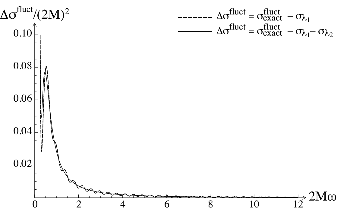
In Fig. 1 are displayed the fluctuations of the total absorption cross section, obtained by subtracting the geometrical cross section of the Schwarzschild black hole, $\sigma_{\mathrm{geo}}=27\pi M^{2}$, from the full sum over the partial waves (3). We also display the contribution of the first Regge pole corresponding to the term $n=1$ in Eq. (13). Both cross sections were obtained by solving numerically the problem defined by (1), (2) and (4) for integer and complex values of the angular momentum. The agreement of the two graphs is remarkable, and we could already consider that the fluctuations of the Schwarzschild absorption cross section around the geometrical cross section are very well described by the first Regge pole contribution. This is further illustrated in Fig. 2, which shows that the difference of the two curves is numerically small with respect to their amplitude in Fig. 1. We also observe that small oscillations remain present in Fig. 2, but they are eliminated by taking into account the contributions of the other Regge poles in Eq. (13). Actually, the contribution of the $n=2$ term is sufficient to explain the effects displayed in Fig. 2. The remaining smooth contribution to $\Delta\sigma^{\text{fluct}}/(2M)^{2}$ comes from the $\mathcal{O}(1/\omega^{2})$ term discussed previously. For high frequencies, it behaves as $\pi/(12\sqrt{3}M\omega)^{2}$.

To end with the Schwarzschild black hole, we now derive a simple formula which describes numerically and physically the fluctuations of the high-energy absorption cross section. Formally, it is valid in the eikonal regime (i.e., for very high frequencies), but we can actually use it even for rather low frequencies. We first recall that the Regge poles of the $S$ matrix, as the associated quasinormal complex frequencies, are due to tunneling near the top of the potential barrier described by (2) (see Refs. [31, 37, 38, 39]). As a consequence, even if it has been obtained for $\omega>0$ and $\ell\in{\mathbb{N}}$ [38, 39], we can start from the formula

where

which provides the absorption probability for a particle when $\omega^{2}\approx V_{0}(\ell)$. Here ${(r_{*})}_{0}$ denotes the maximum of the function $V_{\ell}(r_{*})$ obtained from (2) by using the tortoise coordinate. We now extend (19) to complex angular momenta. It is then easy to show that the singularities of $\Gamma_{\lambda-1/2}(\omega)$ are the Regge poles $\lambda_{n}(\omega)$, with $n\in\mathbb{N}^{*}$, of the Schwarzschild black hole $S$ matrix, given by the approximation [36, 31]

and lying in the first quadrant of the complex $\lambda$ plane, as well as their complex conjugates ${\overline{\lambda}}_{n}(\omega)$ [and obviously also the opposites of both, $-\lambda_{n}(\omega)$ and $-{\overline{\lambda}}_{n}(\omega)$, but they do not contribute to our calculation (9)–(18)]. This result is in agreement with those obtained above and validates the prescription used in order to construct the analytic extension $\Gamma_{\lambda-1/2}(\omega)$ of the greybody factor $\Gamma_{\ell}(\omega)$. Furthermore, we have immediately for the residue (7)

Then, by inserting (21) and (22) into (13), using (11a) and keeping only the contribution of the first Regge pole, we obtain for the high-energy behavior of the oscillating part of the absorption cross section the very simple formula

where $\text{sinc}\,x\equiv(\sin x)/x$ is the sine cardinal. The constant factor multiplying this sinc function involves the geometrical cross section of the black hole $\sigma_{\mathrm{geo}}=27\pi M^{2}$ and the argument of the sinc involves the orbital period, $2\pi(3\sqrt{3}M)$, of a massless particle orbiting the black hole on the photon sphere (see, e.g., Refs. [36, 31, 40]). In fact, the coefficient $8\pi e^{-\pi}$ involves the Lyapunov exponent of the geodesic followed by the particle, but this does not appear clearly here [see our discussion below Eq. (40) for more precision]. In Fig. 1, we have also displayed the eikonal cross section (23). The agreement with the exact result is very good, even for low frequencies. Of course, a more detailed numerical study shows that (23) is actually much less accurate than (13), but it is anyway very nice to have such a simple formula to describe the oscillations of the absorption cross section of the Schwarzschild black hole. Moreover, this formula permits us to interpret naturally the period of the maxima (or the minima, or the zeros) of the fluctuations in terms of constructive interferences of the “surface waves” trapped near the photon sphere (see also Refs. [36] and [31] for related aspects). It is interesting to note that, a long time ago, Sánchez had obtained a fit of the numerical absorption cross section of the Schwarzschild black hole which involved the sinc function of Eq. (23) [10]. Her result was obtained from purely numerical considerations. Here, we have behind formula (23) a powerful and solid theory with a clear physical interpretation, and it can easily be generalized as we shall now see.

We now consider a static and spherically symmetric black hole of arbitrary dimension $d\geq 4$, endowed with a photon sphere. It is defined as the manifold ${\cal M}=\hbox{$]-\infty,+\infty[_{t}$}\times]r_{h},+\infty[_{r}\times S^{d-2}$ with metric $ds^{2}=-f(r)dt^{2}+f(r)^{-1}dr^{2}+d\sigma_{d-2}^{2}$, where $d\sigma_{d-2}^{2}$ denotes the metric on the unit $(d-2)$-sphere $S^{d-2}$. We furthermore assume that $r_{h}$ is a simple root of $f(r)$ and that we have $f(r)>0$ for $r>r_{h}$ and $\underset{r\to+\infty}{\lim}f(r)=1$. We also assume that there exists a value $r_{c}\in\hbox{$]r_{h},+\infty[$}$ for which $f^{\prime}(r_{c})-\frac{2}{r_{c}}f(r_{c})=0$ and $f^{\prime\prime}(r_{c})-\frac{2}{r_{c}^{2}}f(r_{c})<0$. In other words, the spacetime considered is an asymptotically flat black hole with an event horizon at $r_{h}$, its exterior corresponding to $r>r_{h}$, and the assumptions on $r_{c}$ imply the existence of a photon sphere located at $r_{c}$ which is the support of unstable circular null geodesics (see Ref. [32] for more details on these different assumptions). It should also be noted that now the critical impact parameter is given by $b_{c}=r_{c}/\sqrt{f(r_{c})}$ and that the geometrical cross section of this black hole is $\sigma_{\mathrm{geo}}=\pi^{(d-2)/2}b_{c}^{d-2}/\Gamma(d/2)$ (see, e.g., Ref. [16]).

A massless scalar field $\Phi$ propagating on this gravitational background satisfies the wave equation $\Box\Phi=0$, which reduces, after separation of variables and the introduction of the radial partial wave functions $\phi_{\omega\,\ell}(r)$ with $\omega>0$ and $\ell=0,1,2,\dots$, to the Regge-Wheeler equation (1), but instead of (4) we take

and the tortoise coordinate $r_{\ast}$ is now defined from $r$ by the relation $dr_{\ast}/dr=1/f(r)$.

From Eq. (9) of Ref. [41], we can write the corresponding $d$-dimensional absorption cross section of the black hole in the form

where $\Gamma_{\ell}(\omega)$ for $\ell=0,1,\dots$ are the greybody factors defined now by (1), (24), (4) and (5). [The Euler $\Gamma$ function should not be confused with these greybody factors $\Gamma_{\ell}$, bearing a lower index.]

Various equivalent versions of (25) can be obtained by transforming the angular momentum $\ell$ into a complex number $\lambda=\ell+(d-3)/2$ and by constructing the analytic extension $\Gamma_{\lambda-(d-3)/2}(\omega)$ of $\Gamma_{\ell}(\omega)$. In the $d$-dimensional context, we shall consider that

where $T_{\lambda-(d-3)/2}(\omega)$ is the transmission coefficient for the problem defined by (1), (24) and (4) with $\ell\to\lambda-(d-3)/2$. Mutatis mutandis, the properties of $\Gamma_{\lambda-(d-3)/2}(\omega)$ are identical to those of $\Gamma_{\lambda-1/2}(\omega)$ emphasized in Sec. II. In particular:

(i) $\Gamma_{\lambda-(d-3)/2}(\omega)$ is an even function of $\lambda$.

(ii) The singularities of $\Gamma_{\lambda-(d-3)/2}(\omega)$ are symmetrically distributed with respect to the real $\lambda$ axis as well as symmetrically distributed with respect to the origin $O$ of the complex $\lambda$ plane. Furthermore, if we denote as $\lambda_{n}(\omega)$, with $n\in\mathbb{N}^{*}$, those lying in the first quadrant of the complex $\lambda$ plane (the so-called Regge poles), those lying in the fourth quadrant are their complex conjugates ${\overline{\lambda_{n}(\omega)}}$, with $n\in\mathbb{N}^{*}$.

(iii) The residues of $\Gamma_{\lambda-(d-3)/2}(\omega)$ at the poles $\lambda_{n}(\omega)$ and ${\overline{\lambda_{n}(\omega)}}$ are complex conjugates of each other, and we shall denote

In the $d$-dimensional context, it is not possible to sum the series (25) by using one of the usual Poisson sum formula. However, we shall succeed in generalizing (9) by using a modified version of the Sommerfeld-Watson transformation [34]. Indeed, we can write

where ${\cal C}=]+\infty-i\epsilon,-i\epsilon]\cup[-i\epsilon,+i\epsilon]\cup[+i\epsilon,+\infty+i\epsilon[$ (here, we have $\epsilon\to 0_{+}$). We can recover (25) from (IV) by using Cauchy’s theorem and by noting that the poles of the integrand in (IV) are the semi-integers (if $d$ is even) or the integers (if $d$ is odd) $\lambda=\ell+(d-3)/2$, with $\ell\in\mathbb{N}$. Here, it is important to remark that the poles of the function $1/\sin[\pi(\lambda-(d-3)/2)]$ into the interval $[0,(d-3)/2[$ do not contribute because they are neutralized by the zeros of the function $\Gamma[\lambda+(d-3)/2]/\Gamma[\lambda-(d-5)/2]$, which can be written in the form

On the part $[+i\epsilon,+\infty+i\epsilon[$ of the integration contour ${\cal C}$ where $\mathrm{Im}\ \lambda>0$, we can use (11a). On the part $]+\infty-i\epsilon,$ $-i\epsilon]$ of this integration contour where $\mathrm{Im}\ \lambda<0$, we can use (11b) in the form

We can then replace (IV) by

which generalizes (9). The steps leading to (10) and (12) from (9) can be trivially repeated here. We then obtain