July 28, 2010]
Non-equilibrium thermodynamics. II: Application to inhomogeneous systems
Abstract
We provide an extension of a recent approach to study non-equilibrium thermodynamics [Phys. Rev. E 81, 051130 (2010), to be denoted by I in this work] to inhomogeneous systems by considering the latter to be composed of quasi-independent subsystems. The system along with the (macroscopically extremely large) medium forms an isolated system . Starting from the Gibbsian formulation of the entropy for , which is valid even when is out of equilibrium, we derive the Gibbsian formulation of the entropy of , which need not be in equilibrium. We show that the additivity of entropy requires quasi-independence of the subsystems, which requires that the interaction energies between different subsystems must be negligible so that the energy also becomes additive. The thermodynamic potentials of subsystems such as the Gibbs free energy that continuously decrease during approach to equilibrium are determined by the field parameters (temperature, pressure, etc.) of the medium and exist no matter how far the subsystems are out of equilibrium so that their field variables may not even exist. This and the requirement of quasi-independence make our approach different from the conventional approach due to de Groot and others as discussed in the text. As the energy depends on the frame of reference, the thermodynamic potentials and Gibbs fundamental relation, but not the entropy, depend on the frame of reference. The possibility of relative motion between subsystems described by their net linear and angular momenta gives rise to viscous dissipation. The concept of internal equilibrium introduced in I is developed further here and its important consequences are discussed for inhomogeneous systems. The concept of internal variables (various examples are given in the text) as variables that cannot be controlled by the observer for non-equilibrium evolution is also discussed. They are important because the internal equilibrium in the presence of internal variables is lost if internal variables are not used in thermodynamics. It is argued that their affinity vanishes only in equilibrium. Gibbs fundamental relation, thermodynamic potentials and irreversible entropy generation are expressed in terms of observables and internal variables. We use these relations to eventually formulate the non-equilibrium thermodynamics of inhomogeneous systems. We also briefly discuss the case when bodies form an isolated system without any medium to obtain their irreversible contributions and show that this case is no different than when bodies are in an extremely large medium.
I Introduction
I.1 Nature of the Problem
In an earlier paper [1], which we will refer to as I in this work, we have considered some of the consequences of applying the second law of thermodynamics to an isolated system , which consists of a macroscopic system of interest containing a fixed number of particles (atoms or molecules) surrounded by an extremely large medium ; see Fig. 1. From now on, it will be implicitly assumed that the medium is extremely large to be unaffected by the system. (Later in this work, we will also consider to have a fixed volume instead of or fixed and . Furthermore, we will also consider briefly the case of many similar size systems forming the isolated system without the extremely large medium .) The motivation has been to develop this approach to obtain a non-equilibrium thermodynamic description of the open system under various conditions. Throughout this work, we will use body to refer to any of the three kinds systems: the isolated system, the medium or the system. All quantities related to and will be denoted by a suffix , over the top, and without any suffix, respectively. All quantities related to a body will be denoted without any suffix, as if we are dealing with an open system. Similarly, in this work, we will say that the system is open when it is in a medium. Even though it is not the common usage, this should not cause any confusion as the context will be clear.

To avoid complications due to external shear, we had only considered under no external shear in I. This restriction is easily removed as we will do here. The isolated system will still have no external force acting on it to ensure its isolation; see below also. We will now allow forces acting at the surface of the system or any of its subsystems; see Fig. 2(a). These forces must balance the internal stress tensor for mechanical equilibrium. Thus, the force acting on a surface element must equal the stress force (summation over repeated indices implied), and we have [2, 3] for the surface traction force
| (1) |
Here, is the outward unit normal at the surface element surrounding a point on the surface. This condition must be satisfied at every point on the surface The net force and torque acting on the system are given by
respectively; here, for convenience, is taken to be the radius vector of the surface element with respect to the center of mass of the system. The external forces are responsible for the deformation of the system, and also result in the translation and rotation of the system. Let us consider an infinitesimal volume element of mass , which is moving with a velocity and rotating with an angular velocity and has an intrinsic angular momentum . The linear and angular momenta of the system in some fixed frame are given by
respectively; here is the mass of the system ( being the mass of a particle), which we consider fixed for fixed , and and are the location and the translational velocity of the center of mass in this frame. If the frame is taken to be the center of mass frame, then and are zero. If the body as a whole is stationary, then the energy of the body is known as the internal energy. Such a stationary situation was considered in our previous work [1], where no motions were considered. This limitation will be removed here so as to allow for relative motions (translation and rotation) between the system and the medium. These relative motions are the additional sources of viscous dissipation and give rise to additional irreversibility. The irreversibility due to temperature difference (such as between the system and the medium) has already been considered in I.
We should mention here the recent somewhat comprehensive investigation carried out by Bouchbinder and Langer [4] who also consider a system under external shear; however, our approaches and emphases are very different. We should also mention earlier very different equilibrium-like attempts by Lubchenko and Wolynes [5] and by Öttinger [6]. Mention should also be made of a very interesting phenomenological approach by Oono and Paniconi [7] on steady state thermodynamics, which was later advanced by Sasa and Tasaki [8]. The classical local non-equilibrium thermodynamics due to de Donder [10, 9, 11, 12] is close in spirit to our approach and that of Bouchbinder and Langer [4]. It will be the standard formulation with which we will compare and contrast our approach initiated in [1]. Therefore, for the sake of continuity and clarity, we briefly discuss the classical formulation involving local equilibrium in Sect. II. We note that there are other versions of non-equilibrium thermodynamics usually known as the extended, rational and GENERIC non-equilibrium thermodynamics [14, 13]; however, we do not discuss these formulations in this work.
It is well known that the second law of thermodynamics for the isolated system states that
| (2) |
where denotes the entropy of at some instant . It should be stressed that the isolation of requires that there be something outside of from which it is isolated. Therefore, we will assumes that is confined to a finite though extremely large volume [15]. The isolation requires that we neglect all interactions, such as gravitational interactions, of with the outside that cannot be shielded. All interactions with the outside should be relatively very weak to be negligible. All relevant interactions must be confined inside the volume . This to not to be taken as a weakness of our approach as including the interactions with outside will only make an open system, so that our investigation of an open system, which is our primary concern, can then be applied to it.
We should emphasize the following important point. The law of increase of entropy in Eq. (2) should give a pause to those readers who believe that the concept of entropy is meaningful only for an equilibrium state and that the entropy cannot be defined for a non-equilibrium state. This belief is unfounded. The mere fact that the second law dictates the approach to equilibrium clearly implies that the entropy exists even when the system is out of equilibrium. This issue and the related history, in particular the Gibbs formulation of the non-equilibrium entropy, has been reviewed recently [15, and references cited therein], and we refer the reader to this for further details. We should stress that the Gibbs formulation of the entropy requires that the dynamics of the system and that of the isolated system are not deterministic, but rather stochastic; see [15] for further details.
I.2 Important Restrictions in I and Their Removal in the Current Work
An assumption that was implicit, but not stated, in I was that there was no relative motion between the system and the medium and that the isolated system was stationary. This is normally the case in practice in which the various bodies and are stationary in the laboratory frame of reference; the latter we will denote by in this work. In general, one can allow for a translation and rotation of a body, as done here because we now wish to study their effects on the deformation of the system. Because of the stationary assumption, there is no difference between the energy and the internal energy for and . This is a very common but useful assumption as the entropies depend on the internal energies and not on the energies [16]. The latter energies may contain the contribution from the translation and rotation of the system as a whole. In contrast, the internal energies are the energies systems have in a frame in which they are stationary. Whenever we discuss both energies together in the following, the internal energy will be denoted by a superscript ”i” to distinguish it from the energy, which is denoted without the superscript; otherwise, it will be clear which energy we are considering. For a stationary system in the lab frame , the internal energy is the same as the energy. The translation of a body as a whole merely affects the energy, but not its thermodynamic properties. However, the rotation of a body as a whole gives rise to centrifugal potential energy that modifies the energies of microstates and has to be carefully incorporated in any thermodynamic investigation [16, see Sect. 34] as done in Sect. VIII; see also Appendices A and B.
I.3 Present Goal and the Layout
We had focused exclusively on the system as a whole without worrying about its internal parts in I. As entropy palys a central role in our development, we discuss the formulation of entropy and thermodynamic averages in Sect. III, where we show the entropy itself as a thermodynamic average. Under the assumption of internal equilibrium in the system, there were no relative motions between its various parts that could add additional irreversible processes inside the system. In this work, we will remove this limitation and treat the system as inhomogeneous as glasses normally exhibit both spatial and temporal inhomogeneity; see [18, 17, 19] for some recent investigations. We do this by considering to be composed of a collection of a large number of subsystems , which may be different from each other to allow for inhomogeneity and for relative motions and shear forces between different subsystems in terms of internal variables. Each subsystem is still macroscopically large so that we can introduce a legitimate entropy function ; see Sect. X.2 for further elaboration.
Apart from the observables that can be manipulated by the observer, there also appear internal variables often used in describing glasses, as is well known from the early works of Davies and Jones [20, 21]. The latter variables cannot be manipulated by the observer and were briefly introduced in I, but not explored. We will also remedy this situation here and consider glass as an inhomogeneous system with internal variables. Specifically, we treat translations and rotations of various parts of a system as internal variables that are generated by surface traction forces. The alternative approach is to use the traction forces and the strains instead; see for example [4]. The phenomenological ideology introduced by Davies and Jones [20], which has been recently reviewed by Öttinger [6], is by now standard and has been discussed in several textbooks; see for example [22, 23]. The observables and internal variables will be collectively called state variables; see Sect. III for proper definitions of these terms.
In Sect. , we discuss the consequences of internal equilibrium and its similarity with and differences from the concept of local equilibrium [10, 9, 11, 12] discussed in Sect. II. In particular, we argue in the form of Theorem 1 that the system can only sustain a uniform translation and rotation in internal equilibrium. It is assumed here that there are no additional conditions (such as the potential flow in a superfluid) on the velocity. The proof is trivial but the theorem has far reaching consequences. For example, it implies that the uniform rotation must be about a principle axis of inertia. A simple way to understand internal equilibrium is to think of the system as follows. We first disconnect it form the medium with which it is not in equilibrium, and connect it to another medium whose conjugate field variables (, etc.) are exactly the same as that of the system. The system remains in equilibrium with this medium so that there will be no irreversible process in the system. We discuss the generalization of equilibrium Maxwell relation to systems in internal equilibrium. The condition for additivity and quasi-independence is considered in Sect. V, where we prove that the Gibbs entropy formulation in Eq. (21) is also applicable to an open system, which is assumed to be quasi-independent of the medium. Various thermodynamic potentials are identified in Sect. VI that are in accordance with the second law. It is here that we see a clear distinction between our approach and the conventional non-equilibrium theory exploiting the local equilibrium concept [10, 9, 11, 12]. Internal variables are discussed in Sect. VII. We prove that the chemical potential or the affinity associated with an internal variable must be zero when the system is in equilibrium. We also prove that the entropy expressed solely in terms of observables when there are independent internal variables must explicitly depend on time so that while the system is in internal equilibrium with respect to all state variables, it is not in internal equilibrium with respect to only observables. A system undergoing uniform translation and rotation is studied in Sect. VIII where we also develop the Gibbs fundamental relation for such a system. We then apply the results from this study to an isolated system in which the system and the medium undergo relative translational motion in Sect. IX, but the system is homogeneous. An inhomogeneous system with relative motions between its subsystems is studied in the next section. We also discuss in this section the case of several bodies, each in internal equilibrium but different from others, that form an isolated body together by themselves without a medium; see Fig. 2(b). These bodies are macroscopic in size, but are not extensively as large as a medium. We discuss a direct method of calculating the irreversible entropy generation in each body in terms of the equilibrium state of all the bodies. We find that the same results are also obtained by bringing all bodies in contact with a medium as shown in Fig. 2(a). This equivalence is used to prove Theorem 2. All these investigations are extended to include extra observables and internal variables. The final section contains concluding discussion and a brief summary of our results.
II Local Non-equilibrium Thermodynamics: A Brief Review
As entropy is the central quantity appearing in the second law in Eq. (2), we will pay close attention to its determination, although this is usually not done in classical local non-equilibrium thermodynamics [10, 9, 11, 12], where its existence is taken as a postulate with an implicit assumption that it is always additive [9]. The entropy of a system is defined in terms of the local entropy density per unit volume:
| (3) |
The local temperature and pressure are assumed continuous functions of the location and time , and are postulated to always exist. The additivity of the energy results in
| (4) |
Here, is the internal energy, and the translational and rotational kinetic energy density, respectively, and the additional energy contribution due to interactions not included in the internal energy density in a volume of the system; the local mass and angular momentum densities are given by and respectively; compare with Eq. (112) derived later after limiting it to the volume element .
The functional form of the entropy density depends on the nature of the system. For example, for a simple system containing a fixed number of structureless particles, it is assumed to be a function only of the internal energy density and the local number density ; see for example, [9, see Eq. (III.14)]
| (5) |
The local Gibbs free energy density is given by
| (6) |
whether local equilibrium exists or not. (The unconventional use of the symbol instead of will become clear later when we discuss the Gibbs free energy, which follows from the second law and which continuously decrease as the system approaches equilibrium.) However, no direct method of calculating the entropy is given in this approach except by assuming as another postulate the validity of Gibbs fundamental relation, which for a simple system with no internal variables reads
| (7) |
this postulate is a consequence of assuming local equilibrium [9, see Eq. (III.15)]. The presence of the local temperature and pressure in the fundamental relation imposes strong conditions on the nature of the entropy in that its partial derivatives are related to the given and under local equilibrium, which follow from Eq. (7).
We avoid the above issues in the conventional non-equilibrium thermodynamics [10, 9, 11, 12] by first identifying the entropy of the system in terms of microstate probabilities as described below, see Eq. (21), and then use the concept of internal equilibrium to introduce the temperature and pressure in terms of this entropy; the latter are defined only when there is internal equilibrium [1]. This thus avoids the issues inherent in the conventional approach. Our approach is not local in that we always deal with quantities etc. related to macroscopically large systems or subsystems as opposed to the conventional thermodynamics which deals with local quantities etc. As a consequence, not only etc. but also the temperatures, pressures, etc. associated with these systems or subsystems will not always be continuous functions of space at the interfaces. Thus, we will not impose continuity in space on these quantities, which makes our approach distinct from the traditional local non-equilibrium approach of de Donder [10, 9, 11, 12] where these quantities are always treated as continuous. In the latter approach, a system can be broken into subsystems, each sufficiently small, yet large enough to be in internal equilibrium to satisfy Gibbs fundamental relation. This hypothesis is known as the local equilibrium hypothesis. We add another requirement, that of quasi-independence of the subsystems in our approach, which we believe to be extremely important. Only this requirement ensures that the entropy retains the additivity property and also remains a state variable, as we will discuss later in Sect. V.
II.1 Helmholtz Theorem
To accommodate relative motion, we need to allow for surface traction forces , which then give rise to internal forces causing the deformation of the system. These forces can be related to the induced stress tensor as shown in Eq. (1), and will result in a motion of the system due to non-zero net force and torque acting on the system. It is well known that the local motions for a deformable system can be described as a combination of three distinct types of motions [24, 25]:
- (a)
a pure translation
- (b)
a pure strain, and
- (c)
a pure rotation
by expressing the instantaneous difference in the velocity at two nearby points separated by a displacement vector as
| (8) |
where the symmetric tensor
represents the rate of strain tensor and the antisymmetric tensor
is the vorticity tensor, and represents the axial vector associated with The second term in Eq. (8) represents the components of the vector . One should think of as the relative velocity between two neighboring points separated by .
The first contribution represents a pure straining motion while the second contribution represents a rigid-body rotation. For example, a simple shearing motion in which plane layers of the system slide over each other can be treated as a combination of a pure strain (with no rate of volume change) and a rotation [25].
II.2 Stress Tensor
The motion at the local level can also be studied directly by considering the stress tensor. The stress tensor is normally expressed as a sum of the non-dissipative and dissipative or viscous contributions [3]:
| (9) |
in which the viscous contribution is some function that depends on the velocity gradients, i.e., on
Thus, we can express it as
where does not depend on the velocity distribution and is a function of the velocity gradients. For example, in a linear approximation using only , is taken to be
with a constant , which could be conveniently absorbed in In this approximation, we see from Eq. (8) that depends on both the rate of strain tensor and the vorticity .
In general, we can partition into a symmetric and an antisymmetric part, the latter due to the presence of intrinsic rotation of the system [9] and describing the role of the rotational viscosity. Thus, we can also partition into a symmetric and an antisymmetric part. We refer the reader to Chapter 12 in the monograph of de Groot and Mazur [9]. Of course, there may be symmetry reasons such as the isotropy of the system that would forbid the dependence on vorticity, in which case there would be no antisymmetric part. It is possible to show [9] that the rate of change of the intrinsic angular momentum is determined solely by the antisymmetric part of Thus, the absence of this part will imply the conservation of the orbital and intrinsic angular momentum separately.
It can now be shown [9, Eqs. (XII.18) and (XII.18)] that the antisymmetric part
contributes a term proportional to
to the rate of change of the internal energy and to the entropy production. Here, is the vector associated with
and represents the angular velocity of rotation of the system; cf. Eq. (4). Thus, this contribution vanishes for uniform rotation as expected. For , there would be precession of the local volume element [26] about the direction of , so that the rotational viscosity would play an important role until becomes equal to .
II.3 Energy Balance and the First Law
The decomposition in Eq. (9) allows us to break the surface traction also in two terms related to the individual contribution:
where the two new terms are defined similar to that in Eq. (1). The non-viscous contribution is sometimes expressed by taking out the isotropic pressure term as follows
assuming that the thermodynamic pressure can be defined. The rate at which the work is done on the system is given by the average (over all microstates) of the stress tensor at the surface of the system:
| (10) |
where and are the components of and the velocity of the surface element, respectively. When the pressure can be defined, this rate can be expressed as
| (11) |
In this work, we will not consider latent heats and chemical or nuclear reactions within the body. In this case, the rate at which the heat is added to the system is obtained by considering the heat flux through the surface and is given by
where is the heat added to the system in time . We can then write down for the rate of change of the energy due to the dynamics in the system as
| (12) |
which is a restatement of the first law of thermodynamics; see also [4].
It should be remarked that the balance equation (12) is in an integral form for the entire system and should be contrasted with the differential form commonly stated in textbooks; see for example [9]. The latter formulation is valid for infinitesimal volumes. Here, we are not interested in such a local description. Our main focus is to consider regions of the system that are macroscopically large enough so that they can be treated as quasi-independent. Under this condition, the entropy of the system can be approximated to a high accuracy by adding the entropies of the subsystems. We discuss this point further in Sect. IX.1.
II.4 Need for Internal Equilibrium
If the system as a whole is stationary, then the average velocity . In this case, the energy of the system is the internal energy. We will consider this case below in this section for simplicity.
The first law statement in Eq. (12) does not by itself allow us to determine the way the entropy of the system changes. This law is valid even if the system is not in internal equilibrium. In the absence of internal equilibrium, there is no way to determine the change in the entropy from this law. We need to relate with the change in the entropy to determine the latter. However, if we now assume that the system is in internal equilibrium (see I and Sect. below), then the entropy no longer has an explicit -dependence. In this case, we can write down the differential of the entropy of a monatomic system of neutral particles with fixed as [1]
| (13) |
compare this equation with Eq. (7). We can now use Eq. (12) in this equation to determine the rate of change of the entropy. However, as we discuss in Sect. , in this case there is no additional irreversible entropy production arising from viscous stress tensor. Thus, the last contribution in Eqs. (10) or (11) vanishes [27, Sect. 7.4.2]. If there is no shearing at the surface, then the second term in Eq. (11) also vanishes, and we obtain the standard relation
| (14) |
this identification was used in I [1].
II.5 Reversible Entropy Change and Irreversible Entropy Production
We wish to emphasize, as was done in the previous work [1, see Eqs. (16) and (18) in particular] that this assumption of internal equilibrium does not mean that the irreversible entropy production in the system is absent unless the system happens to be in equilibrium with the medium. To see this most easily, we recount from [1] that
| (15) |
is the change in the entropy due to heat transfer to the system that is in internal equilibrium and depends on its instantaneous temperature . We have used the superscript E to indicate that the entropy change we are discussing is due to energy (heat) transfer for which the associated conjugate variable, see Eq. (27), is () and takes the value in equilibrium. It follows from this that the reversible entropy change in the system depends on its equilibrium temperature , which is also the constant temperature of the medium, and is given by
| (16) |
regardless of the instantaneous temperature of the system. This results in [1]
| (17) |
in all cases. Here,
| (18) |
with representing the equilibrium value of the conjugate field associated with the observable , represents the thermodynamic force for the flow of . Since in Eq. (15) undergoes a change due to the heat transfer, the heat transfer is not isothermal. Thus, it should not be surprising that there is an irreversible entropy generation as part of it. On the other hand, the determination of in Eq. (16) requires the heat transfer to be isothermal for the process to be reversible. What is surprising is that is determined not by the current state of the system at , but its equilibrium state in the future so that the concept of causality is inapplicable [15]. It is this particular aspect of that is the cornerstone of the second law of thermodynamics: also depends on the future. We will make use of this observations later.
The situation with other extensive variables like volume is no different. As shown in [1], the entropy change and the reversible entropy change due to a change are given by
| (19) |
It follows from this that the irreversible entropy generation is given by an identical formulation as above for
| (20) |
with given by Eq. (18) with , see also Eq. (28), represents the thermodynamic force for the ”flow” of volume .
It should be stressed that the validity of Eq. (13) follows from the continuity of the entropy and the existence of the internal equilibrium. This is a general relation and is valid for all systems whose macrostate can be described by the three variables and On the other hand, the form of Eq. (14) depends on particular form of the processes that go on in the system. Thus, it is process-specific; recall that we have eliminated various processes in deriving this equation. We can incorporate the missing additional contributions in Eq. (14) by properly introducing internal variables to describe the microstates of the system and generalizing Eq. (13) to include other extensive observables. The issue of internal variables is taken up in Sect. VII, and the generalization of Eq. (13) is taken up in Sect.VIII.
III Entropy and Averages
III.1 Isolated System
The entropy of an isolated system such as , whether in equilibrium or not, is given by the Gibbs formulation
| (21) |
where is the time-dependent probability of the -th microstate of the isolated system ; see a recent review [15] of this formulation for an isolated system, regardless of how far it is from equilibrium. It is assumed that the dynamics of the system is stochastic and not deterministic, as the latter dynamics makes the above entropy a constant of motion in direct contradiction with the second law. In a deterministic, i.e. Hamiltonian dynamics, a microstate uniquely evolves into a microstate, while in a stochastic dynamics, a microstates evolves into several microstates with certain probabilities. The unique evolution is time-reversible, which results in the entropy being a constant of motion. In a stochastic dynamic, the entropy can only increase [15]. Since the system is isolated, we do not allow external forces acting on it; we of course neglect weak stochastic forces acting on it. Thus, any deformation if it occurs is due to internal forces. We have defined the entropy as a quantity, which is equivalent to setting the Boltzmann constant equal to . The collection of these microstates along with their non-zero probabilities represents a macrostate or simply of . As equilibrium and non-equilibrium thermodynamics is an experimental science, a macrostate of any body is specified in terms of a set of some extensive observables that can be manipulated by the observer. The same set of observables are also used to identify the microstates. Most often, the microstates are identified by the energy, volume, and the number of particles that form the elements of , because of their special role in thermodynamics. If there are other extensive mechanical quantities (quantities that are not purely thermodynamic in nature) such as the total linear and angular momenta, then the microstates are characterized by all these extensive quantities, collectively denote by ; see the discussion in Sect. VII for more details. Apart from these observables, a body can also be specified by a set of internal variables [10, 9, 11, 12] that have been found very useful in describing glassy dynamics and will be discussed later in Sect. VII. Indeed, one needs internal variables to also explain the time-evolution of an isolated system towards equilibrium since all its observables remain constant. Thus, the macrostate of the isolated system can use the internal variables for its specification. We will take these internal variables to be also extensive and call both of them as state variables and collectively denote them by . Taking internal variables as extensive allows us to deal all state variables on equal footing, so that generalization from observables to internal variables becomes almost trivial.
Let us continue with the discussion of the isolated system. In general, microstate probabilities are functions of the state variables along with . As a consequence, the entropy is also going to be a function of and . There are situations, when the entropy can also depend on some external parameters such as the angular velocity of the rotation of the frame of reference. These parameters need not necessarily be extensive just as is not. The number of state variables are too limited for a complete microscopic description of the system, but is sufficient to describe the macroscopic conditions of a system.
The observables remain fixed for the isolated system . The internal variable , if present in the isolated system, is normally a function of time; its time-dependence describes the temporal evolution of . While the microstate , hence the value of the state variable in the microstate , does not vary with time, the average for the macrostates varies with :
| (22) |
It should be pointed out that the entropy, as formulated in Eq. (21) is also an average of [15], the negative of the index of probability . There will be times, when we will also use an overbar such as in to indicate such averages for the sake of clarity. For common thermodynamic quantities such as average energy, volume, etc. the normal practice is to not use the overbar (unless clarity is needed) as it is mostly these average quantities that we deal with.
III.2 An Arbitrary Body
It should also be stressed that the microstates for a body remain the same whether the body is isolated or not. We can apply Eqs. (21) and (22) to determine the entropy and the average quantity for any body, isolated or not (such as the system or the medium , neither of which is isolated). In the following, we will always use to denote a microstate of a body but reserve to denote the microstate of the isolated system. The entropy and the average energy of a macrostate of a body is given by
| (23a) | ||||
| (23b) | ||||
| where denotes one of its microstates, whose probability is denoted by . While we can certainly allow microstates with probabilities in Eq. (23), we find it convenient to only allow microstates with non-zero probabilities in the sum. Microstates with non-zero probabilities will be identified as allowed [15] in this work. | ||||
IV Internal Equilibrium Thermodynamics
IV.1 Equiprobability Concept and Consequences: No Internal Variables
We will first consider the case when there are no internal variables. As is the normal practice (see I for details), we assume that the medium is in internal equilibrium even if the system and the medium are not in equilibrium. This assumption is similar to the assumption of local equilibrium in the conventional nonequilibrium thermodynamics noted in Sect. III. As discussed in I and in the review [15], the condition for the internal equilibrium to be met is that the entropy has the maximum possible value at each instant for the instantaneous average value of the observable of the body. For the case considered in I, they are and for the medium; the number of particles of the medium is not allowed to change at all, so that is always kept fixed. It is easy to see from Gibbs’ formulation of the entropy in Eqs. (21) or (23a) that this happens if and only if all the microstates that are allowed () at that instant are equiprobable. Another way to think about the internal equilibrium is to imagine isolating the medium by disconnecting it from the system. This will keep fixed at . Then the entropy of the isolated medium cannot change anymore. In other words, it is in equilibrium. We can apply the same idea to any body in internal equilibrium. The body will remain in equilibrium if it is isolated.
Let us follow the consequences of this concept beyond what was discussed in I.
- (1)
We allow for the possibility of external forces including stresses acting on the system and produced by the medium; see Fig. 1. Under internal equilibrium,
(24) where is the number of allowed microstates [15] at that instant. This immediately leads to the Boltzmann entropy
(25) for a system in internal equilibrium, a common assumption in non-equilibrium thermodynamics; see for example Bouchbinder and Langer [4]. Since the entropy is maximum at each instant , it cannot increase further if all observables are kept fixed at their values at that moment , when the internal equilibrium is achieved. To ensure that is held fixed at , we isolate the system from the medium so that turns into an isolated system. Let its entropy be denoted by after isolation. As the entropy is already at its maximum, it cannot change. In other words, at fixed must be independent of time.
The above argument proves that the entropy has no explicit -dependence when the system is in internal equilibrium:
Its implicit time dependence when is treated as an open system comes from the temporal evolution of . Thus, the (maximum) entropy in Eq. (25) will change with time as changes with time in the open system. For the isolated situation, at fixed will remain constant.
- (2)
Since the entropy is maximum for fixed , there cannot be any additional irreversible entropy production anymore
(26) here, the symbol means that are held fixed.
- (3)
When the system is in internal equilibrium, its various parts must be in equilibrium with each other. Otherwise, there would be irreversible entropy generation.
- (4)
It also follows from (3) that all the arguments that one uses to follow the consequences of equilibrium can be applied to different parts of that are in equilibrium. For example, the arguments that establish that a system in equilibrium can only sustain uniform translation and rotation [16, Sect. 10] can be applied without any change to a system in internal equilibrium. As this result is going to play an important role in our approach, we state it as a theorem.
Theorem 1
There cannot be any relative motion between different parts of for fixed in the state of internal equilibrium. Thus, a system in internal equilibrium can only sustain uniform translation and rotation [16].
Proof. We refer the reader to Landau and Lifshitz [16, Sect. 10] for the details. Their argument applies without any change to an isolated system in equilibrium. We easily extend their argument by considering our system at some instant when it has . We keep fixed at by isolating the system from the medium. The arguments now apply without any change to the system in internal equilibrium. This proves the theorem.
The axis of the uniform rotation must be a principal axis of the instantaneous moment of inertia of the system. Otherwise, the system will undergo precession in space [26] and the rotation will not be uniform.
- (5)
Even with internal equilibrium in the system, there are both elastic and inelastic or plastic deformations [27, Sect. 7.4.2], which result in viscoelasticity in the system.
If and only if the system is under internal equilibrium, the derivatives of with respect to have the significance of the field variables, also called the conjugate variables, which we will denote by or
| (27) |
where denotes all other elements of except the one used in the derivative; compare with Eq. (54). The temperature and the pressure are defined in the customary way by
| (28) |
where denotes all other elements of except or respectively in the two derivatives. The pair of quantities or are called conjugate to each other.
The definitions of the conjugate fields give us an alternative way to interpret the internal equilibrium. We imagine bringing the system in contact with another medium whose field variables are also , where
here denotes the value of the derivative at . To distinguish this medium from the first medium that is characterized by , we denote the first medium by , and the new medium by . The system in internal equilibrium with observables is in equilibrium with the new medium . If the system is isolated by disconnecting it from , then there cannot be any change in the macrostate of the system as all its observables remain constant at . In other words, the system after being isolated remains in equilibrium if it was originally in internal equilibrium, as noted earlier. This will not be true if there are internal variables, to which we will turn to in a moment.
IV.2 Zeroth and the Second Law
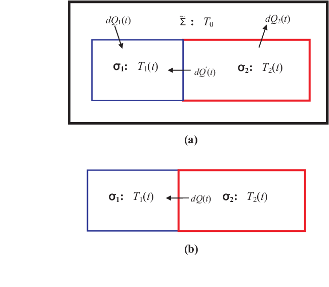
All the above discussion has been for the entire system, but can be easily extended to a system consisting of various subsystems , each in internal equilibrium. Let us consider the system shown in Fig. 2, which consists of two subsystems and whose internal temperatures are and , respectively. Let their respective energies be and , with their sum denoted by . We consider all other observables fixed for both subsystems. We first consider the system to be isolated with no medium, as shown in Fig. 2(b). Then remains constant, but not the individual energies. The irreversible entropy gain for the entire system is
| (29) |
during an infinitesimal heat transfer from the hotter subsystem to the colder subsystem. Here,
plays the role of the thermodynamic force for the isolated system, and should be contrasted with the same quantity for an open system in Eq. (18). As the system is isolated, this is also the entropy change for the system, with
for the two subsystems as follows from Eq. (15). We now consider the system to be in a medium at a fixed temperature , as shown in Fig. 2(a). We take to be the equilibrium temperature of the isolated subsystems; it is intermediate between and . The infinitesimal heat given out by the hotter subsystem is now The heat gained by the colder subsystem must be exactly the heat loss , since we are dealing with an isolated system. Therefore, , so that the entropy of the medium does not change. As the entropy change of the isolated system is equal to that of the system, we have
| (30) |
since . This is the same irreversible entropy gain in Eq. (29) for the isolated system in Fig. 2(b). This should not be surprising as none of the heat transfers is isothermal. Thus, bringing the isolated system , which consists of two subsystems, in contact with a medium, characterized by the equilibrium temperature of , does not affect the irreversible entropy production. It is easy to see that the arguments can be extended to many subsystems and to other field variables. We will not pause here to do that.
At this moment, it is important to follow another important consequence of the thermodynamic force , which vanishes if and only if the system has come to thermal equilibrium. This is the zeroth law of thermodynamics in terms of the internal temperatures of the two subsystems. Thus, the internal instantaneous temperature plays the role of a thermodynamic temperature in that the heat always flows from a hotter subsystem to a colder subsystem. The above result can be easily generalized to many subsystems.
Let us now consider the volumes of the two subsystems to adjust as they come to equilibrium. All other extensive observables are considered fixed. Then the same reasoniong as above results in
where is change in the volume of ; the volume of the isolated system remains unchanged. The corresponding thermodynamic force
vanishes when the system comes to mechanical equilibrium. It usually happens that thermal equilibrium requires mechanical equilibrium in that the forces exerted on each other by any two subsystems must be equal and opposite. Thus, the conditions for the equilibrium is that not only the pressure but also the temperature have the same value in both subsystems.
IV.3 Presence of Internal Variables
We can easily extend the above discussion to include internal variables by replacing by . In the context of internal variables, their conjugate variables are known as ”affinity.” The general form of Eq. (27) is
| (31) |
where denotes all other elements of except the one used in the derivative. The affinity is given by
| (32) |
so that consists of
| (33) |
and . The generalization of the thermodynamic force in Eq. (18) is given by
| (34) |
with representing the equilibrium value of corresponding to the state variable .
Let us now consider the system to be in internal equilibrium, while the medium containing it is , where characterize the medium. If we now disconnect the system from this medium, but bring it in contact with another medium , where and are the field and affinity vectors associated with the system in internal equilibrium, then the system will remain in equilibrium with this medium. This is no different than what we have said above in the absence of any internal variable .
But the situation is very different when we try to keep the system isolated. Since internal variables are not under the control of the observer, they cannot be manipulated to remain constant after isolation and will continue to change. Thus, after the isolation, , the value of at the instance of isolation, will remain constant, but will not remain fixed at its value at the instant it was isolated. This time variation in the internal variables is what drives this isolated system towards its equilibrium state during which its entropy will continuously increase. This is very different from the case above when there were no internal variables. Thus, a system in internal equilibrium cannot be isolated as an equilibrium system if there are internal variables present. It can only remain in equilibrium with the medium .
IV.4 Maxwell Relations
As the concept of internal equilibrium is not that different from the concept of equilibrium, it should not come as a surprise that there are analogs of Maxwell relations. We recall that in equilibrium thermodynamics, the standard Maxwell relations for a system characterized by only and (fixed ) are as follows in terms of Jacobians:
| (35) |
All four Maxwell relations use the same numerators and . They use different denominators. Thus, they can all be combined into one compact relation that can be simply written as
| (36) |
Here, the relation only has a meaning if each side is divided by one of the possible denominators and on both sides.
We now consider a system. For simplicity, we assume that only one internal variable, which we denote by , characterizes this system. We assume the system is in internal equilibrium. To simplify the notation, we will suppress but use the additional variable along with the other two variables. By considering the system in a medium , we recognize that the system is in equilibrium. Thus, the Maxwell relations now for fixed can be compactly represented by
| (37) |
by replacing by which for simplicity have been written as . The extension to the Maxwell relation in terms of the internal variable requires considering the pair in place of or , where denotes the conjugate affinity to . For fixed , the Maxwell relation is
| (38) |
and for fixed , the Maxwell relation is
| (39) |
If we consider the system in the medium , then we have the standard equilibrium Maxwell relations similar to those in Eq. (35). However, we are interested in the possible ”non-equilibrium” Maxwell relations when the system is in the medium . We first consider fixed . The Maxwell relation in Eq. (37) turns into the identity
| (40) |
that is
for the enthalpy and
| (41) |
that is
for the Helmholtz free energy; the details will be given in a separate publications [28]. One can also obtain Maxwell relations at fixed or . For example, we find the following Maxwell relation
that is
Similarly, from the Maxwell relation
we find
The Maxwell relations in Eq. (37-39) contain the internal fields of the system and not of the medium [28] when the system is out of equilibrium. Obviously, the extensive variables in the relation must refer to the system.
IV.5 Internal Equilibrium Thermodynamics versus Local Thermodynamics
We will argue in Sect. V that the concept of internal equilibrium, which we adopt, is no different than the concept of local equilibrium used in Eq. (5) or in the Gibbs fundamental relation in Eq. (7). Despite this, the two approaches based on the concept of local and internal equilibrium, respectively, differ in some important ways that will be elaborated later. Here, we briefly mention these differences. The first important difference is that our approach is truly a statistical mechanical approach for non-equilibrium systems. Once the probabilities of microstates are known, the averages and other moments of all state variables that are used to identify the microstates and the entropy are determined for the macrostate. For example, the average fluctuation in for a body is given by
| (42) |
where
| (43) |
is the average for the body; compare with Eq. (22). As the microstate probabilities exist even when the system is out of equilibrium, these averages including the entropy exist at all times even if the system is not in internal equilibrium. Their temporal variations are controlled by the dynamics governing the system and give rise to various balance equations; see for example Eq. (12). The use of a probabilistic approach in the determination of the entropy and other statistical properties means that the dynamics in the system must be stochastic and not deterministic, as the entropy remains constant in a deterministic dynamics [15]. A consequence of the stochastic nature is that irreversible dissipation becomes an integral part of the statistical description of any system, which then results in the law of increase of entropy as captured by Eq. (2). It is this law that was the foundation of our approach in I, and which we develop further in this work.
The second difference is in the identification of the thermodynamic potentials for the open system, which has been discussed in I and will be further elaborated in Sect. VI and again in Sect. X.2. It is discovered in our approach that thermodynamic potentials contain the field parameters (temperature, pressure, chemical potentials,etc.) of the medium, which determine how far an open system is from its equilibrium with the medium. These thermodynamic potentials satisfy the second law in that they do not increase in a spontaneous process. In contrast, the form given in Eq. (6) for the local Gibbs free energy density or its integral over the volume of the system does not always satisfy this requirement; see the discussion surrounding in Eq. (22) of I. However, there is no discrepancy for the internal energy in the two approaches as both approaches give the same Gibbs fundamental relation. This is because the fundamental relation in both approaches does not depend on the field parameters of the medium, but include the instantaneous field parameters of the system.
The third difference is in the reversible and irreversible entropy changes, which depend on the equilibrium value ( or ) of the conjugate field ( or ), as is easily seen from Eqs. (16), (17), (19) and (20). In the localthermodynamics, these quantities are determined by the local conjugate fields.
The presence of the medium field variable in the thermodynamic potentials of the system does not mean that the situation would be any different if we consider the system or subsystems to form the isolated system without any medium, as shown in Fig. 2(b). In this case, which we consider in Sect. XI.2, we again find that the thermodynamic potentials do not depend on the field variables of the system or subsystems. The role of the field variables of the medium are now played by the equilibrium conjugate variables of the system or subsystems. This then leads us to the following important theorem:
Theorem 2
An isolated system is no different than the open system in an extensively large medium , provided the medium is appropriately chosen to represent the equilibrium state (in terms of ) of the isolated system .
In particular, the reversible entropy change and the irreversible entropy generation in the two cases (a) and (b) in Fig. 2 are exactly the same, as they both depend on the equilibrium conjugate variables of the system or subsystems. An example of this is already seen in Eqs. (16) and (17). We defer the proof of this theorem to Sect. XI.2.
V Additivity of Entropy and Quasi-independence
For simplicity of discussion, we consider all systems to be stationary in this section, so that we only deal with internal energies. It was noted in Sect. III and recently reviewed in [15], the entropy of an isolated body is given by the Gibbs formulation in Eq. (21), regardless of whether it is in equilibrium or not. There is no reason to believe that this formulation also applies to an open body under all conditions, though its applicability in equilibrium is not in dispute [16]. We now prove that this formulation also applies to an open body under a condition that is always taken for granted. We will specifically consider our system at some instant , but the conclusion is valid for all bodies. Let us consider all allowed microstates of with fixed number of particles ; we index these microstates by . Theses microstates correspond to all possible energies and volumes of the system. We use to denote the microstates of whose number of particles is also fixed. A specification of the microstates and gives a unique microstate specification representing a microstate of the isolated system . Hence, the number of microstates of the is the product
| (44) |
where and are respectively the number of all allowed microstates [15] of and respectively at that instant .
As the concept of microstates does not depend on the nature of interactions (they exist even in the absence of interaction), the above equation is valid for all kinds of interactions. Let and denote the internal energies of and , respectively. Let denote the mutual interaction energy between and at that instant. For short-ranged interactions, this energy is determined by the surface of . For convenience, we assume that this entire area is exposed to the surrounding medium, as shown in Fig. 1. If long-ranged interactions are also present, or if the system size is very small, this energy may depend on the entire volume of . In all cases, this energy is defined by the following identity
| (45) |
Because of the smallness of relative to , . If it happens that
| (46) |
we call and quasi-independent. For quasi-independence, the linear size of the system must be at least as large as, but hopefully larger than, the correlation length in the system. In this case, we can neglect their mutual interactions, which is a common practice in the discipline [16]. The quasi-independence of the system and the medium holds to a very high degree of accuracy for all short-ranged interactions [1], provided the system itself is macroscopically large so that the ratio of its surface to volume is insignificant. In most cases, this will also ensure that the correlation length is small compared to the size of the system. If there are also long-ranged interactions, then we can still have quasi-independence provided these interactions are relatively weak and shielding occurs and that Eq. (46) and the condition on the correlation length hold simultaneously.
Let us now assume that and quasi-independent. In this case, the microstates of the two systems are independent of each other to a very high degree of accuracy and we have (we suppress all state variables for simplicity of notation)
Now, using
and the sum rule
we find that
where the two terms in the above equations represent the entropies of the system and the medium
| (47) |
respectively. This demonstration justifies the additivity of entropies
| (48) |
as a consequence of quasi-independence so that
| (49) |
also holds to a very good approximation. Note that we have neither assumed the medium nor the system to be in internal equilibrium in the above demonstration.
If the system and the medium fail to be quasi-independent because their mutual interaction cannot be neglected, then Eq. (46) is violated. In this case, the presence of this interaction acts as a constraint on Consequently, the entropy now will be strictly less than the above entropy in Eq. (48). We denote this difference by [29], which is defined by the following identity
| (50) |
This identity reduces to the above additivity in Eq. (48) provided
| (51) |
compare with Eq. (46). This inequality will in general hold only if the interaction energy is also negligible.
If the strong inequality in Eq. (51) is not satisfied, we have lost the additivity property of the entropy. Let us assume that the strong inequality is satisfied for some large size of the system . Now, as the size of the system decreases, which is what will happen on the way to considering physically infinitesimal volume elements used in Eq. (3), there comes a point where the strong inequalities in Eqs. (46) and (51) are violated. This will destroy the additivity of the entropy as exhibited in Eq. (48).
The violation of entropy additivity occurs at intermediate sizes of the system, somewhere between the macroscopic size where Eqs. (46) and (51) are valid, and small local or microscopic size containing a small number of particles. For example, for the surface to volume ratio for the volume element is about , implying an almost imperceptible error in neglecting the interaction entropy , provided the linear size of this region is large compared to not only to the inter-particle separation [2, p.1] but also the correlation length in the system. Under these conditions, the integrand in Eq. (3) truly refers to a ”physically” infinitesimal volume element containing a very large number of particles. In this sense, our starting premise is similar to that adopted in the conventional non-equilibrium thermodynamics [10, 9, 11, 12]. In particular, our concept of internal equilibrium is no different than the concept of local equilibrium in conventional non-equilibrium thermodynamics, as observed in I, except that we require quasi-independence, which imposes the strong condition that not only the interaction energy be small but also that the linear size be larger than the correlation length. At present, there is some evidence that the correlation length in a glass forming system appears to increasing as the system approaches the glass transition [30].
The discussion above also clarifies that the additivity of entropy is a consequence of the additivity of energy of various parts of the body and that the interaction energies between them must be negligible. This additivity of the energy and entropy was adopted in I. However, as we will be interested in considering parts of as subsystems in this work, the additivity of their entropy requires that their mutual interaction energies be also negligibly small compared to their individual internal energies, and that their linear sizes be large compared to the correlation lengths [30]. These requirements put a strong condition on the sizes of subsystems.
VI Thermodynamic Potentials
VI.1 Fixed Number of Particles of the System
Despite similarities between our approach and that adopted in conventional thermodynamics [10, 9, 11, 12], there were important differences noted in I. One of these was the discovery that the differences of the temperature and pressure of and which are the same as that of and play the role similar to internal variables. The second difference was that the Gibbs free energy in our approach exists even if the system is not in internal equilibrium, and involves the temperature and pressure of or of course,we assume that the medium is in internal equilibrium; see I and Sect. . Under this very weak assumption for the medium, its field variables such as the temperature , pressure , etc. are well defined, and are unaffected by whatever processes happen to be going on within the system or whether is homogeneous or inhomogeneous. When the number of particles in the system is held fixed, the appropriate thermodynamic potential is the Gibbs free energy, which is identified as
| (52) |
where the observables and have explicit time-dependence for fixed . The particular form of the Gibbs free energy is in accordance with the second law in Eq. (2), and remains valid even if the system is so far out of equilibrium that its temperature and pressure cannot be defined; see also Landau and Lifshitz [16, see Sect. 20]. It is not surprising, therefore, that it contains the temperature and pressure of the medium, which are well defined. Theses quantities do not exists for the system unless it happens to be at least in internal equilibrium. Even then, the Gibbs free energy is given by Eq. (52) and contains the temperature and pressure of . As such, it does not represent a state function of the system. In engineering context, this quantity is also known as exergy or availability [31].
However, our form in Eq. (52) differs from the local form of the Gibbs free energy in Eq. (6), which contains the local temperature and pressure. One can argue that the identification of the Gibbs free energy in I was for the entire system, but that once we account for the inhomogeneity by considering subsystems, the Gibbs free energy for each subsystem will somehow become consistent with that in Eq. (6). This is a reasonable possibility and we need to investigate this possibility. This issue is deferred to Sect. X.2.
As the method to identify the Gibbs free energy or other thermodynamic potentials that follow from the second law in Eq. (2) is going to be employed here several times, we briefly sketch the derivation for the sake of continuity. The full details are given in I. We do not assume the existence of the temperature, pressure, etc. of the system to include the situation in our discussion when the system is far away form equilibrium so that they are not defined. For simplicity, we consider a monatomic system of structureless particles under no external shear as in the previous work [1]. Accordingly, we only consider the energy , volume and the number of particles to describe the macrostate of the system at any instant . No internal variables will be considered at this moment. The system and the medium are assumed not to be in equilibrium.
We use the additivity in Eq. (48) to write the entropy of as the sum of the entropies of the system and of the medium. If we also assume that the latter is in internal equilibrium, then we have
| (53) |
there is no explicit -dependence in due to its internal equilibrium. With and fixed, we expand in terms of the small quantities and of the system
where the derivatives are evaluated at . However, as is very close to , there is no harm in evaluating the derivatives at . This is the reason that we have used above for the derivative. This approximation will be made throughout in this work. The error is inconsequential when the system is a very small part of the isolated system. It follows from the internal equilibrium of that
| (54) |
We observe that is a constant, which is independent of the system . Thus,
| (55) |
In terms of
| (56) |
we finally have
| (57) |
It immediately follows from Eq. (2) that the Gibbs free energy of the system in Eq. (52) continuously decreases as the system relaxes towards equilibrium, a result quite well known in classical thermodynamics [16]:
| (58) |
The function continues to decrease and finally becomes identical to the equilibrium Gibbs free energy at the current temperature and pressure . If we abruptly change the temperature and pressure of the system in some state A′, where the system was in equilibrium, to a new state A where the temperature and pressure are respectively, at time , then the initial values of the energy, volume and entropy at the new temperature and pressure remain equal to their respective equilibrium values in the previous state A′ as the microstate probabilities at have not had any time to change. Thus, initially
in the state A; the quantities with a prime are the equilibrium values in the state A′. The Gibbs free energy decreases in accordance with Eq. (58) and eventually becomes equal to its new equilibrium value
where the quantities with the subscript A denote the equilibrium values in the new state A.
It should be noted that the equilibrium Gibbs free energy in the state A′ before the abrupt change is
so that the Gibbs free energy undergoes a discontinuity at due to the abrupt change:
Its magnitude and sign has nothing to do with the second law as the abrupt change is not a spontaneous process.
A similar looking quantity , see Eq. (6) for its local analog in the local non-equilibrium thermodynamics [10, 9, 11, 12],
| (59) |
which can be defined only when the system is under internal equilibrium and not otherwise, was shown to increase with time [1] during relaxation
| (60) |
in a cooling process. Since it does not always decrease with time, it cannot be taken as the Gibbs free energy; the latter is supposed to never increase as the system equilibrates spontaneously as happens with ; see Eq. (58).
VI.2 Fixed Volume of the System
Instead of keeping the number of particles in fixed, let us keep its volume fixed so that the volume of the medium is also kept fixed. The number of particles of the medium is no longer fixed. The entropy of the medium in Eq. (53) is expanded in terms of small quantities and of the system. We follow the steps similar to those above and obtain
| (61) |
where stands for for reasons explained above in deriving Eq. (54). Let us now introduce the chemical potential of the particle in the medium by the standard definition
We thus find that in terms of
| (62) |
which identifies a different thermodynamic potential in this case as
| (63) |
this thermodynamic potential also uses the field variables of the medium. We should emphasize again that no assumption about the internal equilibrium of the system has been made. The system may or may not be in internal equilibrium. The application of the second law in Eq. (2) now gives
| (64) |
VI.3 Fixed and of the System
If both and are kept fixed, it is easy to follow the above derivation to conclude that the Helmholtz free energy
must continuously decrease as the system reaches equilibrium:
Thus, the second law for an open system is expressed in terms of different thermodynamic potentials depending on which variables are held fixed.
VII Internal variables
As said above, a suitable equilibrium macrostate description of the system requires a set of independent macroscopic observables that can be controlled by an experimentalist and whose values will allow the experimentalist to differentiate between different macrostates of the same system. It normally happens that experimentalists have a far less number of external controls than the possible extensive variables that can be used to characterize the macrostates. Thus, one does not characterize a macrostate, especially an equilibrium macrostate, by specifying all of the relevant extensive system quantities. For example, for a single component system, one normally uses and to specify the macrostate if there are no external shearing forces. Let us for the moment consider a system without external shear. Usually, one considers a system with fixed ; then and can be controlled by the two external variables and associated with the medium. However, these external variables need not necessarily control the local or internal structures in the system at all times during its evolution towards equilibrium. As Frenkel has observed, the local structures can be important when considering the structural relaxation in a glass or other non-equilibrium systems [32, p. 208]. For example, one can consider the average numbers of neighbors and next-neighbors of a given particle to describe the local structure in the system. These quantities multiplied by the number can play the role of internal variables. The corresponding conjugate variables, normally identified as ”chemical potentials” or ”affinity” for these internal variables usually vanish in equilibrium. Frenkel goes on and calculates viscoelastic effects due to structural changes and compares them with Maxwell’s model of elastic relaxation or an RC-circuit. This investigation by Frenkel [32] shows that internal variables can play an important role in the temporal evolution towards equilibrium in some systems such as glasses. As such, they become an integral part of the description of any non-equilibrium system and determine the relaxation of the system [2, Sect. 78]. The internal variables are also called hidden variables or internal order parameters.
To introduce the concept of internal variables, let us consider our isolated system for which one can identify a set of conserved quantities, i.e. integrals of motion. For a mechanical system of degrees of freedom, the number of such integrals of motion are [26]. Of these integrals of motion, those that are additive play an important role in thermodynamics and statistical mechanics. The notable ones are the energy, and linear and angular momenta of the system, among others such as the polarization, magnetization, etc. For the moment, let us consider to be stationary. Its macrostate is characterized by fixed internal energy , volume , particle number and other extensive observables, collectively denoted by . All these observables are constant for . Let us consider the energy , which is an integral of motion. It usually happens (see below for an example) that there are many different components of the energy whose total sum is the energy of :
| (65) |
where is the number of energy components. It is that is a constant of motion, not the individual components ; the latter will continue to change as the system evolves in time while maintaining Eq. (65). Let denote the number of microstates corresponding to the macrostate at time . At each instant , the microstates in can be partitioned into groups according to the possible values of . Because of the sum rule in Eq. (65), only of the components are independent for a given , which we take to be given by . We will denote this set by an -vector whose elements are. Then,
Let denote the number of microstates for a given . These microstates define a new macrostate, which we denote by . Obviously,
| (66) |
the sum is over all possible . As the system evolves, different components of evolve in time , but and remain fixed. Thus, a better understanding of the evolution of the system can be obtained by monitoring how the various components change in time. For this, it is better to use to identify the macrostate even though individual cannot be controlled by the observer. As can be controlled by the observer, it is still the choice observable to be used for identifying a macrostate. This is even more true for the isolated system for which is a constant of motion. The components of then play the role of internal variables in developing non-equilibrium thermodynamics of the isolated system.
It is evident that the same ”extended” description should also be useful for an open system . The only difference between an open system and an isolated system is that not all elements of remain fixed. Some of the observables, denoted by are controlled by external field parameters (such as ,, etc.) of the medium so that they do not remain fixed but continue to fluctuate about their mean that keeps changing in time. However, at least one of the extensive observables such as must be kept constant to quantify the size of the system [33]. Thus, for an open system, these observables can be replaced by the fields , with the remaining observables remaining constant. We will denote the latter observables by to remind us that they are constant. The open system can be either specified by or . However, for the sake of convenience, we will continue to use rather than or . Let us now consider which is not in internal equilibrium so that it undergoes internal deformation due to relative motions between its various parts. If there are external strains on the system, they can be controlled by us from the outside. Hence, they will not be considered as internal variables. However, internal stresses acting on various parts of the system when there are no external strains on the system are beyond our control and must be treated as internal variables in describing the system. As said earlier, we can describe the internal forces acting on each part in terms of translation and rotation of its various parts; see Sect. II.1. These motions must be described by the use of suitable internal variables such as the linear and angular momenta, as was discussed in Sect. I.2.
As the internal variables are uncontrollable, their affinity in equilibrium must vanish as we prove now as a theorem.
Theorem 3
The affinity of an internal variable must vanish in equilibrium.
Proof. It is sufficient to prove the theorem for an isolated system. Also, we will prove it for the energy components in Eq. (65). The extension to the general case is a trivial extension and will not be done here. As we are dealing with equilibrium, we consider equilibrium values of all the quantities, which are going to be represented by suppressing the argument as they are stationary. We now construct the following partition function for the isolated system
where is the the -vector equilibrium affinity. Such a partition function correctly describes the situation in which the internal variables are not constant but keep changing from microstate to microstate. We now observe that this partition function reduces to the equilibrium value in Eq. (66) (where we take the limit ), provided :
for each of the internal variable in the set . This proves the theorem.
The above theorem deals with equilibrium affinities, and says nothing about the affinities of the internal variables when the system is out of equilibrium.
Let denote one of the microstates associated with the macrostate and one of the microstates associated with the macrostate . Then, using their probabilities and we can determine the entropy of the two macrostates using the Gibbs formulation in Eq. (21):
| (67a) | ||||
| (67b) | ||||
| For a macroscopically large system, the following standard statistical mechanical arguments can be used to highlight the maximum of the summand in Eq. (66). Let the maximum of the summand be denoted by , which occurs for some particular value of | ||||
We separate the maximum contribution from the sum and rewrite Eq. (66) as follows:
where the sum is over all remaining . It is normally the case that the ratio in the above sum is vanishingly small for a macroscopic system and that the sum can be neglected. In this case, we have
| (68) |
For a macroscopically large open system such as , the above equation is formally valid, except that we must replace by which stands for , and by :
| (69) |
We now prove an important theorem about the nature of the entropy.
Theorem 4
The entropy expressed only in terms of the observables when (independent) internal variables are present must explicitly depend on
Proof. We first consider the isolated system and prove the theorem for it. For to be independent of (fixed) , it must surely have an explicit dependence on time. In other words, must be a function of and . Let us assume that there is an explicit -dependence in both -functions in Eq. (68). As the entropy of the macrostate is given by the sum over all microstates in Eq. (23a), it must explicitly depend on . Thus, the theorem is satisfied. If, however, neither of the -functions in Eq. (68) have any explicit -dependence, then this is possible only if becomes a function of as the left side is only a function of . Since is constant, itself must be constant. The latter is the situation in equilibrium:
| (70) |
It follows that is no longer an independent variable when the system is in equilibrium. Obviously, this case is not covered by the theorem since is not independent. The entropy in this case is given by the Boltzmann formulation, cf. Eq. (25), and we have from Eq. (68)
Let us now consider the special case when the macrostate satisfies the condition of internal equilibrium. In this case, does not explicitly depend on and should be written as with having an explicit time dependence. This entropy is again given by Eq. (25):
| (71) |
It now follows from Eq. (68) that must have an explicit time-dependence due to the explicit -dependence of in . This is because different values of will result in different values of , which can be treated as associated with the macrostate at different times. This is the first case considered above. Thus, will have an explicit -dependence even though does not.
This proves the theorem for an isolated system.
Let us consider an open system such as . Again, must be a function of and to remain independent of . Let us assume that there is an explicit -dependence in the -functions in Eq. (69). As the entropy of the macrostate of is given by the sum over all microstates in Eq.(67a), it must explicitly depend on . If, however, neither of the -functions have any explicit -dependence, then becomes a function of . In this case, it is not independent of . This situation is then not relevant for the theorem.
The possibility in which is independent of , but has no explicit -dependence, when the system is under internal equilibrium, is very important. Fixing allows us to think of the system as an isolated system. Now, we can use the argument given above for the isolated system to conclude that different values of will result in different values of , which can be treated as associated with the macrostate at different times. In other words, the macrostate does not represent an internal equilibrium state. Thus, we conclude that a macrostate under internal equilibrium results in a macrostate ; the latter is, however, not in internal equilibrium.
This proves the theorem.
It follows from the above discussion that a general thermodynamic state can be taken to be a function of internal variables along with other observables and time when we deal with non-equilibrium states. For an open system in which many of the observables are controlled by external field parameters (such as ,, etc.) of the medium, we can express either as
or as
Away from equilibrium, the internal variable differs from its equilibrium values , and is normally treated as an independent variable and plays an important role in the dynamics of the system as the latter strives to reach equilibrium. Thus, it is not surprising that internal variables are employed to specify the macrostate of a glass. In non-equilibrium thermodynamics, this fact has been recognized for quite some time [10, 9, 11, 12].
Internal variables can also be related to the presence of internal degrees of freedom in the particles of interest. The internal degrees are more common in polymers but can also occur in small molecules in the form of rotation about some internal axes. An example will clarify the point much better. Consider a polymerization process resulting in a system of polydisperse linear polymer chains of average molecular weight in a solution [34]. The model is defined on a lattice of sites and volume , with a constant representing the volume occupied by a lattice site. One normally uses , , defined below in Eq. (72), and the number of chains as the standard observables that can be used to identify the macrostate (equilibrium or not) of the polymer solution. In turn, these quantities are controlled by the temperature, pressure and the initiation-termination and propagation rates; the last two can be related to the initiation-termination activity controlling the number of endgroups, two for each polymer, and the middlegroup activity. These activities determine the corresponding affinity or ”chemical potentials.” Let denote the number of monomers, each monomer occupying a lattice site, in terms of the number of voids or sites not covered by monomers so that
| (72) |
In terms of the number of middle groups or , the number of chemical bonds in the polymers is given by
There are two kinds of energy in the model [34]. One kind of energy is due to mutual interactions of voids (v) with the end (E) and middle (M) groups, and the mutual interactions between chemically unbonded M and E. Let v,M or E, denote the number of nearest-neighbor contacts , and the corresponding interaction energies, respectively. The other kind of energy is due to intrachain gauche bonds (g), and hairpin turns (hp). Their energies are for gauche bonds and for hairpin turns; here and denote the number of gauche bonds and hairpin turns and parallel bonds and and are their energies. In addition, there is a mutual interaction energy between two parallel (chemical) bonds, which may belong to the same or different polymers. Let denote the number parallel bonds, each of energy . Thus,
| (73) |
where we have introduced and with obvious definitions. We thus observe that the energy can be partitioned into six extensive energies, five of which can be taken as internal variables.
To summarize, we conclude that the quantities that cannot be controlled by the observer can be identified as the internal variables. This statement should not be taken literary as what is considered uncontrollable today may not remain so in the future. Thus, to some degree, the decision to identify the internal variables is left to the observer. For us, any variable that cannot be controlled to have a fixed value when the system is out of equilibrium will be taken as an internal variable [35]. It should also be noted that the number of internal variables is not a unique number for a given system. For example, to describe local structures in a monatomic system [32], one can consider any number of neighboring particles (neighbors, next-neighbors, next-to-next neighbors, and so on). Thus, a choice will have to be made to see how many of them are useful in a given experiment or investigation. This certainly gives rise to an additional complication in the study of non-equilibrium system.
Our approach allows us to associate affinity in a formal sense with all internal variables. This is how the classical non-equilibrium thermodynamics has been developed [10, 9, 11, 12]. As observed by Landau and Lifshitz [2], the use of internal variables in a modern way can be traced to Mandelstam and Leontovich [36]; see also Pokrovski [37]. Under the internal equilibrium assumption, Prigogine addresses the issue of internal variables (orientation of a molecule, deformation due to flow, elastic deformation, etc.) in Sect. 11, Chapter III of his classic book [12], or in Sect. 10.4 in the modern version [11], and couples them to their ”chemical potentials” or affinities. Indeed, Prigogine and Mazur were the first one to do this in their classic paper [38]; see also Coleman and Gurtin [39]. The issue of the internal variables is also discussed in Sect. 6, Ch. 10 in [9]. Pokrovski [37] provides a very illuminating discussion of internal variables and their role in determining the internal energy. Thus, we will treat internal variables as additional thermodynamic extensive quantities or ”observables” similar to the number of chemical species in chemical reactions that can be controlled by affinities or chemical potentials. More recently, the idea has also been visited by Bouchbinder and Langer [4].
VIII Thermodynamics of a simple rotating body
VIII.1 General Case
We will find it convenient for later use to consider observing a body in different frames of reference; see also Appendices A and B. For concreteness, we consider the system and assume that no internal variables and no other observables besides the energy, volume and number of particles are present; the latter can be added easily as we will discuss later. We will consider three special frames: the lab frame denoted by , an intermediate frame , with its axes parallel to those of and moving with respect to with a velocity , and a frame with its origin common with and rotating with respect to it with an angular velocity . Let denote the location of the origins of and in the lab frame at time with Let denote the coordinate of a particle of in the frame, and its velocity in this frame at time . Its coordinate in the lab frame is given by
| (74) |
its velocity is given by Eq. (138). As shown in the Appendix A, the energy of the particle in the two frames are related as shown in Eq. (141). Let us consider to be the frame in which the center of mass of the body is at the origin. we will call it the center of mass frame for the body. Then, applying the above two relations to all the particles in the system and averaging over all allowed microstates [15], which is carried out later in Sect. VIII.3, we obtain that the energy of the system in the three frames are related as shown in Eqs. (147) and (150):
| (75a) | ||||
| (75b) | ||||
| where and are introduced in Eq. (144). We have not used the overbar to express the statistical averages as explained in Sect. VIII.3 but is implied. | ||||
We first prove the following theorem:
Theorem 5
The entropy of a system is the same in all three frames ,, and .
Proof. To prove the theorem, we proceed as follows. Only for simplicity of the argument and presentation, we focus on a system with fixed and at some instant . The extension to considering other extensive variables is trivial. Consider observing the system simultaneously at in these frames. It is evident that corresponding to each pair of the coordinates and momenta of a given particle in the lab frame at this moment, there is a unique pair and in the other two frames. This is true of all the particles. The collection of positions and momenta of all the particles defines a point in the phase space. In classical statistical mechanics, a microstate of the system is identified by a small volume element of size about a point in the phase space. Thus, corresponding to each microstate ( or ) in one frame, there exists a unique microstate in the other two frames. The uniqueness of microstate-mapping ensures that their probabilities in the three frames are also equal:
| (76) |
Let us consider all the microstates of the same energy in the frame at time , and let denote their number and the set of their probabilities (not to be confused with momenta , etc.). Because of the uniqueness of the mapping of these microstates noted above, not only the number of microstates in the three frames are the same at that instant
but also the set of their probabilities
however, their energies are different as given by Eqs. (75)(75a) and (75b). This immediately shows that the entropies using the general Gibbs formulation in Eq. (21) are equal in the three frames:
| (77) |
whether the system is in internal equilibrium or not. This proves the theorem.
VIII.2 System under Internal Equilibrium
We now specialize and assume the existence of the internal equilibrium, so that all microstates are equally probable
| (78) |
Hence, the three entropies are each equal to
| (79) |
It follows from Eq. (77) that there is no reason to use different subscripts to distinguish the entropies. Accordingly, we will use to represent the entropies in different frames; their energy arguments will of course depend on the frame of reference. The arguments and above are actually external parameters that are not extensive. We will show below that the entropies in the and frames are actually functions of extensive quantities and that are conjugate to and , respectively; cf. Eq. (27).
VIII.3 Statistical Averaging over Allowed Microstates
We now investigate the consequences of statistical averaging over microstates with non-zero probabilities [15] and show that its consequences are the same as expressed in Eqs. (75) and (77). We first note that in Eq. (144) depends on the coordinates and momenta of the particles, but this is not the case with , even though both are extensive quantities. As in Eq. (147) or (75a) is for a microstate determined by the coordinates and momenta of the particles, we need to average it using microstate probabilities in Eq. (78). Averaging over various microstates relates the average energies in the two frame. We use an overbar, see Eqs. (22) and (43), to denote the average. We find that the same form also describes the desired relation between the average energies:
| (80) |
where
| (81) |
The momentum , of course, does not require any averaging as noted above. Eq. (80) is valid at each instance . We can also take the statistical average of Eq. (145a) to obtain
| (82) |
where the two sums are over all the particles in the system. Here and are the instantaneous position and velocity of the th particle in a microstate with respect to the frame; we have suppressed the subscript from and for the sake of notational simplicity. In the last equation, the third contribution is due to the relative motion of the particles with respect to the frame. Indeed, the average of Eq. (146) immediately yields
| (83) |
The third contribution in Eq. (82) and the first contribution in Eq. (83) vanish when the system is in internal equilibrium because of the absence of any relative motion in that case; see Theorem 1.
Since also does not depend on the velocity , a similar averaging of Eqs. (151) and (152) gives us
| (84a) | ||||
| (84b) | ||||
| Comparing the above equations with the equations in the Appendix B, we see that there is no reason to make a distinction between , used in the proof above, and or the average energies and the energy used above in the proof. This justifies not using overbars to indicate statistical averages in Eq. (75). | ||||
Since the entropy in Eq. (79) is fixed for fixed and we can express the above two derivatives at fixed instead of fixed :
| (85) |
The above equation is similar to the well known result [16, Sect. 11] in equilibrium statistical mechanics that the statistical average of the derivatives of the the energy with respect to external parameters ( and ) should be taken at constant entropy and other extensive quantities. We have extended this result to internal equilibrium now. Introducing the following standard derivatives
| (86) |
defining the temperature and pressure of the system, we can write down the following differential identity
| (87) |
It should be noted that because of Eq. (84a), the average energy does not depend on the velocity of the frames and . Thus, there is no reason to keep fixed in the various derivatives in Eqs. (84-86).
For
we find that
| (88) |
which is an extension of the result given in Landau and Lifshitz [16, Sect. 26] to the internal equilibrium. The point to note is that the entropy in the frame is a function of the conjugate variable instead of . However, for
we also find an additional contribution due to :
| (89) |
given in terms of all extensive quantities. The additional contribution due to the momentum differential is due to the velocity of the system as a whole and is important to include in the lab frame. For example, such a contribution is needed to describe the flow of a superfluid in which the normal and superfluid components have different velocities so that the superfluid cannot be considered at rest in any frame [2, see Eq. (130.9)]. We will need to allow for this possibility when we extend our approach of nonequilibrium thermodynamics to inhomogeneous systems where different subsystems will undergo relative motion. It follows form Eq. (89) that the drift velocity of the center of mass of the system is given by
| (90) |
Similarly, the angular velocity is given by
| (91) |
We again observe that the entropy in the lab frame is a function of the extensive conjugate quantities and rather than the external parameters and .
From now on, we will not use the overbar to show statistical averages for the sake of notational simplicity.
It is clear from Eq. (87) that we must treat as a function of and for constant . Alternatively, we must treat as a function of and
| (92) |
which is identical to the functional dependence shown in Eq. (77), except that we no longer have an explicit -dependence because of internal equilibrium. The important point to observe is that the entropy is a function of not only the energy in the frame, but is also a function of the angular velocity of the reference frame when rotation is involved.
VIII.4 Same Temperature and Pressure in Different Frames
We now make an important observation. It follows from Eqs. (88) and (89) that
| (93) |
obtained by differentiating with respect to Similar equations are obtained when we differentiate with respect to
| (94) |
These equations are identical to the derivatives in Eq. (86) and show that the internal temperature and the internal pressure are the same in the three frames. Moreover, it is the same entropy function that appears in Eq. (87) also appears in Eqs. (88) and (89). In other words, the entropy is the same in all frames, except that the arguments are different.
IX Thermodynamics Potentials and Gibbs Fundamental Relation for a Homogeneous System with Translational Motion
IX.1 Thermodynamic Potentials for a System under Arbitrary Conditions
IX.1.1 Fixed number of particles of the system
Before we discuss the inhomogeneous case, let us consider the homogeneous situation considered in I and revisited briefly in Sect. VI, and extend it to the case when the system moves as a whole with a linear momentum . We still assume that is at rest. Because of the linear momentum conservation, the linear momentum of the center of mass of is . Thus, the centers of mass and are moving towards each other. For simplicity, we will assume the absence of overall intrinsic rotation for and individually. This can easily be incorporated as we do in the next section. Then we only need to consider the orbital angular momentum of in terms of the locations and of the centers of mass of and , respectively. It is clear that always vanishes since the centers of mass of and are moving towards or away from each other so that and are colinear :
The (average) internal energies of and in their center of mass frames (the frame) are
while and denote their total energies in the lab frame , respectively; see Eq. (75). However, because of the extreme large size of , its mass satisfies the inequality , so that we can replace bywithout any appreciable error. The entropy of is a function of the internal energy however, this is not relevant for our argument here if we are only interested in identifying the appropriate thermodynamic potential for the system. The energy
of remains constant in time. As discussed above, the additivity of energy is valid under the assumption that the interaction energy between the system and the medium is negligible. This ensures that the entropies are also additive. In the lab frame , the entropies of the and are obtained by considering their entropies in respective rest frames and they are and , respectively; recall that we have set for each of them.
Using the fact that the medium is under internal equilibrium, we modify Eq. (53) to reflect the dependence on internal energies to obtain
| (95) |
We now expand and follow the steps in arriving at Eq. (55); the steps are unaffected by the motion of . We thus obtain
in terms of the energy and volume of the system. We can now identify the Gibbs free energy and enthalpy in the lab frame in terms of the energy of the system:
| (96) |
compare with the Gibbs free energy in Eq. (52). Thus, the second law in terms of the Gibbs free energy remains unchanged and is given by Eq. (58).
In the center of mass frame of the system, the Gibbs free energy and the enthalpy of the system are given by
| (97) |
Note that the above functions depend on the internal energy and not the energy of the system . But they are not useful in the lab frame in which the system is being observed. Thus, we conclude that the overall motion of the system does not change the enthalpy and the Gibbs free energy; we must use the appropriate energy in the frame of observation; the temperature and the pressure of the medium are not affected by the choice of the frame as noted near the end of Sect. VIII. Similarly, the entropy of the system is unaffected by the choice of the frame as shown by Theorem 5.
IX.1.2 Fixed volume of the system
Let us assume that instead of keeping fixed, we keep the volume of the system fixed. Then following the procedure given in Sect. VI, we find find that the correct thermodynamic potential now in the two frames and are given by
respectively.
IX.1.3 Fixed and of the system
Let us assume that we keep and fixed. Then following the procedure given in Sect. VI, we find find that the correct thermodynamic potential now in the two frames and are given by the Helmholtz free energy
respectively.
IX.1.4 Extension to many state variables
From now on, we will list energy, volume and particle number for any body separately and use and to denote the rest of the observables and state variables, respectively. We will only fix the number of particles but allow all other state variables to fluctuate. In this case, in Eq. (95) must be written as and its expansion in terms of small quantities gives
Here, corresponds evaluating the derivative at ( and so that these derivatives are constant, independent of the properties of the system; see the discussion in deriving Eq. (54). Introducing the corresponding ”chemical potential vector” for and the ”affinity vector” (see Sect. VII) for because of the internal equilibrium of
| (98) |
we can identify a new thermodynamic potential
| (99) |
in the lab frame . As and are constant, we have
because . Thus, is a constant, and the second law tells us that
| (100) |
as expected in any spontaneous process. In the frame, we will instead have
| (101) |
The important point to note is that chemical potential vector and the affinity vector are associated with the medium, just as are. The analogue of the thermodynamic potential and are
respectively. Again, it follows from the second law that
| (102) |
as expected in any spontaneous process.
IX.2 Gibbs Fundamental Relation for a System under Internal Equilibrium
IX.2.1 No extra state variables
We will first assume that there are no internal variables, but the system satisfies the condition of internal equilibrium so that no longer depends explicitly on time. Then, we can identify the temperature, pressure, and the chemical potential of the system by
| (103a) | ||||
| (103b) | ||||
| (103c) | ||||
| This allows us to write down the Gibbs fundamental relation for constant as | ||||
which can be rearranged to write down the first law of thermodynamics
| (104) |
We now turn to Eq. (80). In terms of the momentum of the center of mass frame of the system, we have
| (105) |
recall that according to our assumption, the system has no intrinsic angular momentum. This allows us to use Eq. (104) to write down the differential form
| (106) |
for the first law of thermodynamics in terms of the energy rather than the internal energy . This has some important consequences and will be extremely useful in the following. The first consequence is that it allows us to think of as a function of four variables :
This equation is the Gibbs fundamental relation relating the entropy with rather than . The second consequence, which follows from the Gibbs fundamental relation is that
| (107a) | ||||
| (107b) | ||||
| (107c) | ||||
| (107d) | ||||
| The drift velocity (of the center of mass) of the system is given a thermodynamic interpretation in terms of the derivative in Eq. (107b) at fixed and . For the case when the number of particles is held fixed, and the last term in and will be absent. For fixed , the third term in and will be absent, and so on. | ||||
IX.2.2 Inclusion of state variables
In the presence of internal variables and , the extension of the above relations is quite obvious. Introducing the instantaneous chemical potential vector associated with and the affinity vector associated with using
| (108) |
we generalize the entropy differential to
| (109a) | ||||
| (109b) | ||||
X Inhomogeneous System with Relative Motion
X.1 Subsystems undergoing Relative Motion
We now consider the isolated system to be stationary so that it has no linear and angular momenta. However, and may have relative motion so that they each may possess linear and angular momenta that individually must cancel out:
| (110) |
Moreover, we will now treat as inhomogeneous and assume that it can be decomposed into a collection of a large number of subsystems , which may be in different macrostates to allow for inhomogeneity and for relative motion between different subsystems and within each subsystem. Each subsystem is still macroscopically large so that we can not only introduce a legitimate entropy function for the macrostate via Gibbs’s formulation
where denotes one of the allowed microstates of the subsystem corresponding to the macrostate characterized by observables and , but we also have these entropies satisfy the additive property
| (111) |
which requires their quasi-independence as discussed in Sect. V at each instant . Using the entropy we can introduce the appropriate thermodynamic functions, but care must be exercised in identifying these functions in the lab frame , where the experiments are done. This is because the energies depend on the frame of reference, which will result in different values of the energies and thermodynamic potentials in different frames, such as the lab frame and the rotating frame frame attached to the center of mass of , which is translating with a linear velocity and rotating with an angular velocity .
To make further progress, we will make another assumption later as we did in I that each subsystem is in internal equilibrium. This occurs when all microstates contributing to the entropy are equiprobable
here represents the number of microstates of the subsystem at time . Under the equiprobability assumption or the internal equilibrium assumption,
which is what one would obtain by applying the Boltzmann formulation of the entropy [15]. It also follows from Theorem 1 that the entire subsystem is uniformly translating with a linear velocity and rotating with an angular velocity so that the system in internal equilibrium is stationary in the frame .
X.2 System under Arbitrary Conditions
The internal energy for each subsystem is related to its energy in the lab frame
| (112) |
see Eq. (80). Alternatively, we can use Eq. (82) to express this relation as
| (113) |
where each sum is over particles in the subsystem . The third term in the last equation vanishes when the subsystem is in internal equilibrium as commented earlier. We also have the additivity laws
| (114a) | ||||
| (114b) | ||||
| (114c) | ||||
| at each instant . The angular momentum is the orbital angular momentum of with representing the location and momentum of the center of mass of , respectively, and should not be confused with its intrinsic angular momentum introduced in Eq. (144). We should emphasize that the additivity of the energy requires that the interaction energy between subsystems be negligible. This condition is necessary for the entropy to be additive as discussed in Sect. V. As a consequence, we do not have the contribution analogous to in Eq. (4). This distinguishes our approach with that taken in local non-equilibrium thermodynamics [10, 9, 11, 12]. | ||||
We keep fixed for simplicity so that is also fixed, and allow and to vary in time. We assume as above that has well-defined field variables (, etc.) which do not change with time. This is ensured by assuming internal equilibrium for the medium. This is the only assumption we make regarding the isolated system for which we have
Because the medium is taken to be in internal equilibrium, its energy is related to its internal energy according to Eq. (80)
| (115) |
where according to Eq. (110), we have taken , and where is the moment of inertia of the medium about its axis of rotation. The axis of rotation must be one of its principal axis of rotation; see the comment after the proof of Theorem 1 in Sect. . The contribution coming from the internal motion, which is similar to the third contribution in Eq. (113) applied to the medium vanishes because of its uniform translation and rotation following Theorem 1 applied to the medium. The contribution similar to the last term in Eq. (113) is the standard rotational kinetic energy of the medium treated as a rigid body. The angular momentum is given by
Assuming that the motions are finite, we conclude that must be finite. Therefore, for an extremely large medium, and must be extremely small, which ensure that the last two terms in Eq. (115) are extremely small. This allows us to approximate
| (116) |
without any appreciable error. As far as the system is concerned, the relationship between its internal energy and the energy is still given by Eq. (147)
| (117) |
except that the system may not be uniformly translating and rotating about any of its principal axis of inertia. We take and as constants, but allow for and ( and ) to change with time. Now, we use the entropy additivity
and expand
by treating and as small parameters; here, corresponds to evaluating the derivatives at ( and ). We have also used the definitions of the field variables of the medium in terms of the derivatives of the entropy in Eqs. (54) and (98), and set as established in Sect. VII. We thus finally obtain
where
Observe that the expansion of does not require any knowledge of what is happening with the system . For example, we have not assumed internal equilibrium in the system or any of its subsystems. Since is a constant as established earlier, the second law tells us that
| (118) |
the desired result for the system. The inhomogeneity of the system has no relevance in the above conclusion.
Let us now assume that and introduce
| (119) |
for the subsystem . It is clear that
Because of the quasi-independence of various subsystems, Eq. (118) immediately leads to
| (120) |
Thus, can be identified as the Gibbs free energy of the subsystem in the lab frame . Comparing this definition with the definition in Eq, (6) used in the conventional non-equilibrium thermodynamics, we see that the discrepancy in the two Gibbs free energy has not disappeared by taking into account the inhomogeneity inherent in the system.
It may be argued that the above identification of in Eq. (119) is based on considering the entire system in contact with the medium. One can alternatively consider a particular subsystem of the system in contact with the medium and the remaining subsystems. However, a little bit of reflection shows that this will not affect the behavior of for the simple reason that the remaining subsystems still form a very small part of the isolated system so that they cannot affect the internal equilibrium of the medium. To see this more clearly, let us introduce a new medium consisting of and the remaining subsystems. Only for the sake of simplicity, we do not consider any additional state variables. The argument can be easily extended to include them. Let denote the entropy and and the internal energy, volume and the number of particles of , the latter of which is kept fixed. Expanding this entropy in terms of the small quantities and of the chosen subsystem requires calculating the derivatives
Because of the small size of the system relative to the original medium , these derivatives are not different from
respectively. Thus, using for the energy of the subsystem , we find that
Using this in , where is the angular velocity of the frame of the selected subsystem, allows us to identify
| (121) |
as the Gibbs free energy of the particular subsystem . It now follows from Eq. (2) that
a property we expect from the Gibbs free energy of a system. Incidentally, this also provides an independent justification of the inequality in Eq. (120).
X.3 System under Internal Equilibrium
The above derivation only uses the second law, and the assumption that the medium satisfies the condition of internal equilibrium. The situation with the first law is very different. In general, the differential of the entropy of the subsystem is given by
cf. Eqs. (77) and (92). If we now assume internal equilibrium so that does not have an explicit -dependence, we can get rid of the last term above. In this case only, the remaining derivatives identify the field variables etc. of the subsystem
| (122) |
These derivatives then allows us to obtain the Gibbs fundamental relation
| (123) |
Using
we find the first law of thermodynamics can be expressed in terms of the energy as
| (124) | ||||
compare with Eq. (89). This allows us to think of the entropy as a function
so that the drift and the angular velocities in internal equilibrium are given by
| (125) |
However, different subsystems will undergo relative motions with respect to each other as and are different for them. In addition, their temperatures and pressures are also different for each other, and so are and . Thus, there would be viscous dissipation and, consequently, entropy production as they come to equilibrium with each other and with the medium. We now turn to this issue.
XI Reversible and Irreversible Contributions
XI.1 General Considerations: Bodies in a Medium
It is a well-known fact [16, Sect. 10] that in equilibrium, the system has a uniform translational motion as a whole with a constant velocity and a uniform rotation of the whole system with a constant angular velocity . Thus, there cannot be relative motions between different subsystems in equilibrium. Thus, no internal macroscopic motion is possible in equilibrium. In equilibrium, the coefficients of the differential quantities in Eq. (124) take their constant values of the medium. Writing
| (126) |
as a sum of the change in the entropy due to reversible exchange with the medium and the production of the entropy due to irreversible processes within the system, we have
and
| (127) | ||||
| (128) |
where
| (129) |
is the difference of the conjugate field at time and its value in equilibrium, i.e. as , and represents the thermodynamic force associated with the conjugate extensive quantity ; see also Eq. (18). For the internal variables, the equilibrium value of is zero. According to the second law of thermodynamics, not only but each term in Eq. (127) is non-negative:
where and form a conjugate pair. In terms of these pairs, we can express the two parts of the entropy as follows:
| (130) |
which is the general form of the entropy differenmtial and its two components.
Let us now turn back to the current case under investigation. We can express the generalized Gibbs fundamental relation as
where
and
The generalized form for the Gibbs fundamental relation is evidently
where represents all state variables except the energy , and where and .
It is easy to see that performing the Legendre transform to obtain the Gibbs free energy in Eq. (119) only affects the form of but leaves unaffected. Thus, it is easy to see that
where
and
The general form of is
where represents all state variables except the energy and the volume .
XI.2 Bodies forming a Finite Isolated System without a Medium
So far, we have considered a system or a collection of subsystems in a very large medium so that its field variables are held fixed at . We now consider a collection of bodies of comparable sizes forming an isolated system . In this case, we cannot treat any of the bodies as a (macroscopically extensively large) medium with a fixed field at . As the collection strives towards equilibrium, their field variables continue to change in time. This causes a problem in identifying reversible contributions to various quantities. To solve this problem, we discuss below a simple case; the generalization to more complex situation will be obvious.
XI.2.1 Two Bodies
Let us consider the simplest possible case of two comparable bodies and in internal equilibrium at temperature and , respectively, that are brought in thermal contact at time We will simplify the discussion by assuming that all other extensive observables besides the energy are held fixed. The case of two bodies in the shape of rectangular cuboid along the -axis are shown schematically in Fig. 3(a), with the rectangular interface of area lying in the -plane.
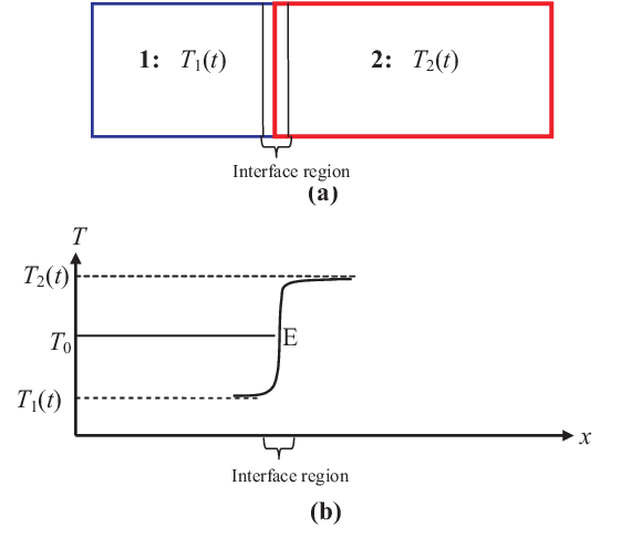
Let be the infinitesimal heat given to the body by the body . As the amount of heat is infinitesimal, it does not alter the temperatures of the bodies in any significant way so that the entropy of the isolated system changes by
at .; compare with Eq. (29). This expression will not be correct as time goes on as the temperature continues to change. The general expression for the irreversible entropy generation is
| (131) |
where is the infinitesimal heat given to the body by the body between and , and are the instantaneous internal temperatures of the two bodies. It is clear from the discussion following Eq. (29) that the irreversible entropy generation in Eq. (131) is the sum of entropy changes in the two bodies. Thus, Eq. (131) is exact for the isolated system consisting of the two bodies. However, the point to remember is that it is the irreversible entropy generation in the two bodies, and says nothing about the irreversible entropy generation within each body.
If the system above were not isolated, then Eq. (131) would still give the entropy change due to the direct flow of heat between the two bodies, but it not represent the irreversible entropy generation due to this heat flow. Moreover, there would also be changes in the entropy of the system and each of the bodies due to heat exchange with the medium or other bodies. These entropy changes will also have their own irreversible entropy generations. The presence of the medium at the equilibrium temperature of the isolated system is discussed below. The situation when is not the equilibrium temperature of the isolated system is very different, as discussed later; see the discussion after Eq. (132).
What can we say about the irreversible entropy generation within each body? This question is, to the best of our knowledge, is not answered within the local thermodynamics approach. To answer this question in our approach, we proceed as follows. We know that the entropy generation in each body must vanish when the bodies come to equilibrium. To obtain the desired result, we introduce the common temperature , when the two bodies come to equilibrium. We now discuss two alternative approaches to determine the individual entropy generation on the way to prove Theorem 2.
Introduction of a Medium at constant
Let us imagine that we insert the two bodies in an extensively large medium kept at a fixed temperature , with all three bodies now forming a new isolated system . The situation is schematically shown in Fig. 4. There is no direct contact between the two bodies, as shown. Despite this, the heat loss by the body to is completely transferred to body . An alternative is to insert the medium between the two bodies along the -axis but not surrounding them from all sides with the same effect of transferring the entire heat from body to body . The width of the medium along the -axis may be infinitesimally small of order , but must have a macroscopically large cross-sectional area in the -plane to ensure its constant temperature at all times. In either case, the entropy of the medium does not change so that , and Therefore, the irreversible entropy generation in the new isolated system is identical to the irreversible entropy generation in . This artificial introduction of can now be exploited to obtain the irreversible entropy generation in each smaller body. The method of calculation above can be easily applied to this case, see Eq. (127), to yield
| (132) |
where is the heat addede to body or given out by body . By comparing with Fig. 2, we note that , giving
It is evident that these entropy productions vanish in equilibrium, as required by the notion of equilibrium between the two bodies. If we had introduced a medium held at a constant temperature , then the equilibrium will occur at , and not at , and we would end up with a different final state of than that of . Thus, the medium must have the constant temperature .

The situation will be very different if the medium is taken to be at a themperature . In this case, the heat given to body is different from the heat given out by body . Comparing with Fig. 2, we note for the total amount of heat given out by and the total amount of heat given to that , giving
The irreversible entropy generation in the two bodies are now givem by
so that is given by
| (133) |
Notice that for and . Similarly, for and . Thus, each of the last two irreversible entropy generation contributions above is non-negative, as expected. We will see below that the last two contributions are absent in the local theory.
The above approach can now be extended to many bodies at different initial temperatures . We assume that the medium surrounds all the bodies so that there is no direct contact between the bodies. If still denotes the final temperature of all the bodies, treated as an isolated system , then the medium must be chosen to be also at the same constant temperature . It is obvious that
| (134) |
where denotes the infinitesimal heat added to the -th body between and and is its instantaneous internal temperature; compare with Eq. (127). This is a generalization of Eq. (17) to many bodies, and exploits the absence of causality inherent in , as exemplified by Eq. (16). The irreversible entropy generation in the isolated system consisting only of the bodies (without the medium) is the sum of all these contributions:
as it must be for an isolated system; Obviusly, does not depend on the final temperature . Here, we have used the fact that
because of the isolation of and . It is quite clear that the discussion is easily extended to include other extensive variables which results in the expression for , which is identical in form to the expression in Eq. (127).
One may feel uneasy that the introduction of the fictitious medium has changed the problem. To see that this is not the case, we reemphasize that its introduction does not affect the heat . Since, it is the heat that determines the entropy generation, and since the equilibrium state of each body is the correct equilibrium state, the result must be correct. To offer an even stronger argument, we now provide an alternative proof without the introduction of the medium so that we can feel comfortable in associating a medium in the case when finite-size bodies form an isolated system. The importance of this trick is that it allows us to use all the results we have found by the use of a medium.
Without any Medium
Let us revert to the simple case of two bodies in thermal contact. In reality, the interface or the contact region between the two bodies is not a sharp boundary with a discontinuity in temperature; rather, it is a narrow region of width over which the temperature rapidly changes from to , as shown in Fig. 3(b). Thus, there exist a point E over this region where the temperature is precisely . It is possible that the location of the point E along the -axis changes with time, but this point is irrelevant. The relevant point is that the temperature in a very narrow width around and including this point will remain constant in time. If we take the narrow neighborhood of a point whose temperature is different from , its temperature will eventually change to , as equilibrium is achieved. Thus, the temperature of the narrow region around this point will not be constant in time. We take the region where the temperature is greater than along with the half-width around E on the side of to be the part of the body , while the region with the temperature less than along with the half-width around E on the side of to be the part of the body . From the quasi-independence of the two bodies, it is clear that the inclusion of these regions will not significantly affect the internal temperatures to The heat lost by the body is transferred to the body at a constant temperature . Thus, while
where is the internal temperature of the body ,
so that
as discovered above; see Eq. (132). In a similar fashion, we obtain
in accordance with Eq. (132).
The above discussion justifies the use of as a temperature in the interfacial region. However, the important point is that the determination of for any body requires the use of the equilibrium temperature of the body in accordance with Eq. (16). Thus, the discussion is equally valid for any number of subsystems in the system.
Comaprison with Local Thermodynamics
The same result as in Eq. (131) is also obtained in the local thermodynamics, as can be easily seen; see for example [12, Eq. (3.14)]. In the limit in which the interfacial region between the two subsystems is infinitesimal in width along the -direction, we can obtain the continuum analog of the irreversible entropy generation between the two neighboring regions. Denoting by and by we have
for conduction. Dividing and multiplying by the cross-sectional area of the interface, and using as the volume of the interfacial region, we have for the rate of entropy production per unit interfacial volume
| (135) |
where denotes the heat flux. This expression (in three dimensions, the result will contain ) in this limit is a standard result for the entropy production due to heat conduction in local thermodynamics.
It should be stressed that our derivation of above is independent of the how long the two subsystems are along the -axis, but assumes implicitly that has a Taylor series expansion. It is also obvious that must be zero outside the interfacial region. Thus, should be correctly identified as the rate of entropy per unit volume in the interfacial region. Therefore, as it follows from the discussion immediately following Eq. (131), the derivation says nothing about how much of the irreversible entropy is generated within each body. The issue is avoided in local thermodynamics by assuming that the entire volume of the system is composed only of such interfacial regions. This is contrary to the basic postulate of local equilibrium according to which each local region has a well-defined temperature , while the interfacial regions have non-zero gradients of the temperature.
We also observe that the form of in Eq. (135) is only valid for the case when Eq. (131) is valid. It is not valid for the case covered in Eq. (133). This is the case when the equilibrium temperature of the system is different from the equilibrium temperature of the two bodies under consideration if treated as isolated bodies. Thus, the above expression will not be valid if our system consists of a large number of bodies so that the irreversible entropy generation between any two bodies in contact will be given by Eq. (133). In this case, the expresasion explicitly contains the equilibrium temperature of the system in the last two terms, which is not the case with in Eq. (135), thus verifying the earlier statment made after Eq. (133).
XI.2.2 Several Bodies
Let us now consider a simple extension of the case shown in Fig. 3(a) in which there are several bodies B in thermal contact along the -axis forming an isolated body , with their temperatures in an increasing order: . Let again denote the equilibrium temperature of the isolated body , so that there exist a point E over their interface region where the temperature is precisely . Let us consider the infinitesimal heat received by to be the part of the heat that was given out by the body and was transferred unaltered via to Any heat transfer through the interface region at constant is isothermal. Therefore, the reversible entropy change due to is precisely . The entropy change of is so that it immediately follows that
as above. Similarly, we find
for the body B, where is the heat rejected by B, which was transferred isothermally to the body unaltetred. For the body , which receives an infinitesimal heat , we similarly find
and so on. All these results can be easily obtained by inserting a medium held at fixed temperature at the interface between each connsecutive pair of bodies. Thus, we conclude that we can consider an isolated inhomogeneous body as a body embedded in a medium without affecting any of the consequences. This then proves Theorem 2.
XI.3 General Discussion
XII Discussion and Conclusions
We have proposed a scheme to extend our previous work in I to an inhomogeneous system in which subsystems may undergo relative translational and rotational motions with respect to each other to contribute to irreversibility. Another source of irreversibility is the temperature variation, which was considered in I. Each subsystem or the medium is identified by a set of extensive state variables , and some constant parameters , some of which may be external parameters and need not be extensive. Examples of may be the number of particles in the system that characterize the system, or the translational and the angular velocities of the frame of reference in which the observations are made. Examples of the state variables are mechanical quantities such as energy, volume, etc. and the internal variables are the translational and angular momenta of the various subsystems, etc.
XII.1 Quasi-independence and Additivity of Entropy and Energy
As our approach starts from the second law, the law of increase of entropy, the entropy as a state function plays the most important role in our approach. Accordingly, we need to ensure that this quantity can always be determined by or at least formally defined in terms of some basic quantities pertaining to the macrostate of the system of interest. We use the Gibbs formulation of the entropy such as that in Eq. (21), which is applicable in all cases as discussed in a recent review [15]. This formulation is well-established for an isolated system [15], but we show in Sect. V that it is also applicable to an open system even when it is not in equilibrium with its surrounding medium. This formulation of entropy for open system is a well known result in equilibrium thermodynamics [16] and our demonstration generalizes this result to non-equilibrium systems so that this entropy can be used as the central quantity in developing a non-equilibrium thermodynamics with the second law as the starting point. It is required that the open system be quasi-independent of the medium. We have shown in Sect. V that this quasi-independence is a very important property, which is required for the additivity of the entropy and of energy. For example, quasi-independence of the system and the medium ensures that their energy of interaction is negligible so that dropping it makes their energies additive, as seen from Eqs. (45) and (49). Indeed, without the additivity of the energy, the entropy cannot be additive as discussed in Sect. V. The basic idea is very simple but profound. The entropy being a state function must only depend on state variables. By definition, all state variables of a body must be solely determined by what happens within the body. If there are other bodies, their influence on the body must not destroy the additivity of all extensive state variables. Let us consider the isolated system consisting of the system and the medium it is in contact with, which is considered in Sect. V; in particular, consider the energies in Eq. (45). We will assume no relative motion between and the medium to make the discussion simple. The energies and then represent the energies of the isolated system, the system and the medium, respectively. However, the presence of the interaction energy in this equation destroys the required property that the right side of Eq. (45) is the sum of internal energies of the system and the medium; the interaction energy is a property of both bodies. Accordingly, the entropy of cannot depend only on the energies of the two bodies separately. The difference represented by in Eq. (50) depends on both bodies. Thus, the entropy of the isolated system cannot be a sum of entropies, each representing the entropy of one of the bodies alone. In other words, generalizing this result to a collection of bodies bj forming a body B, we conclude that the entropy B of B cannot be expressed as a sum of entropies, each term b representing the entropy of the body bj
However, the additivity requires not only that the sum of the energies of various parts bj of a body must yield the energy of the body B itself
which is satisfied if the linear sizes of the bodies are large compared with the range of interaction, but also requires that various bodies are quasi-independent, which is satisfied if the linear sizes of the bodies are large compared with thecorrelation length. Unless thess properties hold, the entropy cannot be expressed as a sum of the entropies of its parts, with each entropy depending only on the properties of the part alone. It is the latter property that makes entropy a state function.
XII.2 Concept of Internal Equilibrium
For a body (or its parts, such as subsystems) out of equilibrium, the entropy usually has an explicit dependence on time in addition to the implicit time-dependence
the latter arises from the dependence of the entropy on state variables and that explicitly depend on time; we will suppress this time-dependence in the following for notational simplicity. (We will assume, as discussed in [33], that at least one observable, which we take to be the number of particles is held fixed and is not contained in .) Thus, such an entropy will continue to change (increase if the body is isolated) for fixed state variables. For a homogeneous body, this will happen if the state variables in and do not uniquely specify its state. In other words, there may be other internal variables not contained in . This is a connsequence of a simple generalization of Theorem 4. The other possibility is that the body is not homogeneous. If the isolated body is not in equilibrium, its entropy continues to increase according to the second law in Eq. (2). However, if it happens that the entropy of the body does not explicitly depend on time
then its entropy must be at its maximum for fixed and . This is how we had introduced the concept of internal equilibrium in I: in this state, the entropy of a system, which is not in equilibrium with the medium , has no explicit time-dependence. It can be brought in contact with another medium , representing the medium , so that it remains in equilibrium with the new medium. In other words, there is no difference between a body in internal equilibrium with the medium , and the body in equilibrium with the medium ; in the latter case, the medium ensures to keep the averages and fixed. In both cases, the entropy is maximum for the fixed values of their state variables and . Accordingly, all properties of a body in equilibrium also hold for a body in internal equilibrium at each instant. For example, Theorem 1 established in Sect. II.4 shows that there cannot be any relative motion within such a body. The only possible motion is a uniform translation and a rigid-body rotation. As a consequence, as discussed in Sect. II.4, there is no viscous dissipation within the body in internal equilibrium. Thus, while there is no relative motion between the system and , there will in general be relative motions between the system and the medium . This result can be generalized to the following statement: The only source of viscous dissipation in a collection of bodies is then due to relative motions between different bodies, when each of which is postulated to be in internal equilibrium.

It was assumed in I that the system at each instant remains in internal equilibrium as it goes from one equilibrium macrostate in contact with a medium at time to another equilibrium macrostate in contact with a medium as . Let us try to understand the behavior of its entropy during this process, which can then be extended to a subsystem in internal equilibrium. The field variables for the two macrostates are and , respectively. As discussed several times, the intermediate macrostate at some instant can be thought of as an equilibrium state of the system in contact with a medium after being disconnected from the medium . In this equilibrium state, the system has a well-defined field and the entropy , which is shown by the solid curve in Fig. 5. However, this equilibrium state of the system does not represent the equilibrium state of the system in contact with either the medium or the medium . If we bring the system in contact with the medium its entropy will increase as the internal variables relax towards the new equilibrium, to be denoted by with fixed . The equilibrium entropy of the system in will be denoted by , which is shown by the dotted curve in Fig. 5.
Because of our assumption of internal equilibrium, represents the maximum possible entropy for the macrostate at . The change in the entropy is given by
where is the equilibrium entropy in the macrostate at , and is shown by the left-most arrow in Fig. 5. The total entropy change in the entire process is
where as the equilibrium entropy in the macrostate as .
The entropy difference can always be broken into two parts in analogy with the two terms in eq. (126):
with see the right-most arrow in Fig. 5, representing the entropy exchange with the medium and the irreversible entropy production within the system, see the middle small arrow in Fig. 5. It does not matter whether the process is reversible or irreversible, the entropy change is always . In the former process, , and . In the latter process,
and there is irreversible entropy production during the passage from to ,
in accordance with Eq. (128). We thus see that irreversible generation of entropy has been accounted for in our approach; see also I and Eq. (128). We can easily extend the above discussion to the subsystems, where we now also have the possibility of irreversible entropy generation through relative motions between them, which is also accounted for in our approach.
We have found (Theorem 4) that while a body is in internal equilibrium in the presence of internal variables, it is not in internal equilibrium when internal variables are not considered in its description. In other words, the entropy of a body, see the solid curve for in Fig. 5,
| (136) |
has no explicit time-dependence; however, it becomes an explicit function of time if expressed only in terms of observables:
| (137) |
This theorem shows how important the internal variables are in describing glasses. Because of the presence of , this entropy will continue to increase and approach , shown in Fig. 5, if we keep fixed.
As experimentalists can only control the observables in , it is the expression of the entropy in Eq. (137) that is experimentally relevant. Because of the explicit -dependence, the body will continue to relax even if the observables are held fixed by isolating the body from its surroundings and bringing it in contact with the medium . This relaxation occurs because the internal variable is no longer held fixed. It will continue to change with time until finally the entropy reaches its maximum possible value for fixed . We can apply Theorem 3 for an isolated system to our body. The conclusion is that the maximum of the entropy occurs when for the internal variable is identically zero, which is why we had selected this particular medium. The final value of is some value . The body in this equilibrium state is the fully relaxed body with its entropy given by
this entropy is shown as in Fig. 5. The affinity of the internal variable is identically zero, and the fields in this state are given by . This equilibrium state of the isolated body should not be confused with the state of the body in internal equilibrium in the presence of the internal variable , as shown in Eq.(136). This body has different from , and the corresponding affinity different from zero.
XII.3 Thermodynamic Potentials
The additivity of the entropy and energy allows us to treat our system as a collection of quasi-independent subsystems so that we can develop the thermodynamics of an inhomogeneous system. Under the mildest possible assumption that the medium is in internal equilibrium so that its field variables are defined via Eq. (98), but the system itself is (or the subsystems are) not necessarily in internal equilibrium, we are able to identify the thermodynamic potential for the system. The field variables of the system in internal equilibrium vary with time and, therefore, they differ from the medium’s field variables. They become identical only when the system is in equilibrium with the medium. It is obvious from Eq. (98) that the product
is dimensionless because the entropy is defined as dimensionless in this work. Accordingly, the (dimensionless) entropy can be expressed in terms of these dimensionless products. It follows then that resulting thermodynamic potentials will contain these products, as shown in Sect. X.2. The actual form of the thermodynamic potential function depends on the choice of the set , and requires field variables to maintain the dimensions of each term appearing in it. The fields variables in the thermodynamic potentials are the field variables of the medium, and not of the system as the latter are not even defined when the system in not in internal equilibrium; see for example, Eq. (56) or (63). This is true whether we consider the system or any of its many subsystems; the latter are considered in Sect. X.2. This is surprising since one knows that, in equilibrium thermodynamics, the thermodynamic potentials are state quantities. Therefore, they must contain all quantities related to the system. It just happens that in equilibrium the field variables are identical to the medium’s field variables. Therefore, our thermodynamic potentials reduce to the standard thermodynamic potentials in equilibrium. In this case, they become state functions. But this is not true when the system is not in equilibrium. What is surprising is that this result remains true even when the system or subsystem is in internal variable. The thermodynamic potentials always contain fields of the medium and not of the system or subsystem. These functions have the required thermodynamic property that they can never increase in any spontaneous process, as seen from Eq. (100) or (102). One can easily see that this property is a consequence of the convexity property of the thermodynamic potentials. In contrast, a function obtained from thermodynamic potentials by replacing medium’s fields by the body’s field, when the latter is in internal equilibrium, does not have this required thermodynamic property. An example of this is the function or from or given in Eq. (6) or (59).
While each subsystem is in internal equilibrium, so that there can be no irreversible processes inside them, the irreversibility occurs due to relative motions going on among them. Because of the internal equilibrium, each subsystem has its own internal temperature , pressure or other conjugate field variables. How are these temperatures and pressures related to the internal temperature and pressure introduced in I? To answer these questions, we consider their definitions in the frame:
see Eq. (122) for the definition of and . Let us first consider the temperature. Introducing
we have
Thus, we have
Introducing
we find that
The same exercise can be carried out for other state variables. Introducing
for the -th state variable , we find that
XII.4 Contrast with Local Non-equilibrium Thermodynamics
Our approach differs from the traditional local non-equilibrium thermodynamics due to de Groot [10, 9, 11, 12], briefly discussed in Sect. III, in three important ways.
- 1.
The first one relates to the principle of additivity of energy. The energy in the local non-equilibrium thermodynamics is not the sum of the energies of its various part due to the presence of the mutual interaction energies expressed by as seen from Eq. (4). Indeed, usually one applies local equilibrium to a volume element , what is traditionally called a physically infinitesimal volume in that, while it contains a large number of atoms, the corresponding volume is still infinitesimally small. Such a volume is conventionally called a ”particle” (not to be confused with our usage which refers to an atom or molecule). For all practical purposes, it is indeed considered as a limit . It is evident that one must then consider the interaction energy to account for the interaction of this volume with the rest of the system. Thus, the local non-equilibrium thermodynamics takes the additivity of entropy is taken as postulate even when the energy is not additive.
- 2.
Because the volume element is treated infinitesimal in the local theory, all thermodynamic quantities are also treated as continuous in space, while this continuity is not a prerequisite in our approach.
- 3.
Our approach also differs from the local non-equilibrium theory in the form of the thermodynamic potentials. The volume element is considered to be in internal equilibrium from the start so that it has a well-defined temperature, pressure, etc. These fields are used in identifying the thermodynamic potentials. For example, the Gibbs free energy of the ”particle” is taken to be even if the system consisting of such ”particles” is not in equilibrium with the medium.
- 4.
Another imporatnt difference between the two approaches is that the reversible entropy change and the irreversible entropy generation in each subsystem also depends on the equilibrium state of the system. The irreversible entropy generation in the local theory depends only on the current local properties.
These differences make our approach very different from the local non-equilibrium thermodynamics due to de Groot [10, 9, 11, 12].
Acknowledgements I would like to thank Arkady Leonov for a discussion on the local non-equilibrium thermodynamics and him and Peter Wolynes for their suggestion to apply the approach of I to inhomogeneous systems. I would also like to thank an anonymous referee of I who wanted the current approach to include internal dissipation.
Appendix A Relation Between Lab and Body Frames
Let us consider a particle of mass in the lab frame , where it has a velocity and the potential energy . The Lagrangian in this frame is given by
Let us transform to a rotating frame which is moving with a velocity and rotating with an angular velocity The velocity of the particle in is given by and is related to according to
| (138) |
where is the coordinate of the particle in the frame, and is related to the coordinate of the particle in the lab frame by
In the following, it would also be convenient to consider a nonrotating frame , which is only moving with the velocity with respect to the lab frame, but whose origin coincides with that of . The Lagrangian in the frame is given by
| (139) |
in which we have omitted , which is a total time derivative.
The canonical momentum is obtained as
so that the energy of the particle becomes
| (140) |
Expressing in terms of from Eq. (138), we find that
| (141) |
where
| (142) |
Incidentally, we also note that
Thus,
which explains why there is no need to use or as a subscript in .
Appendix B A Rotating and Translating System
Let us now extend the previous calculation for a single particle to a system of particles of total mass at a given instant . The system is also characterized by the number of particles and its volume. For specificity, we use and to denote these quantities. The notation should not mean that we are only considering the system here. The system we have in mind is any generic system. We assume that this system is translating with a velocity and rotating with an angular velocity as a whole, both of which can change in time. For notational simplicity, we will suppress the explicit -dependence of various quantities here. We focus on one particular instant . We take the center of mass of this system to coincide with the origin of , so that is fixed to the body and rotating with it. In this case, represents the center of mass frame. We now sum Eq. (141) over all particles, with the result that it is replaced by
| (143) |
where we have introduced
| (144) |
Here, is the intrinsic angular momentum of the system of particles in the frame. The summation in the above formulas, which are also applicable to non-uniform rotation and translation of the center of mass frame , is a sum over all the particles in the system. The value of in the frame represents the internal energy of the system. The equation (143) generalizes the result given by Landau and Lifshitz [26, see their Eq. (39.13)] to the case when The present generalization is not limited to constant rotation and translation.
We can express as follows:
in which the second sum on the right vanishes for , the center of mass frame. For the same reason, the third term in the second equation in Eq. (140) does not contribute to the energy of the system. Thus, we find
| (145a) | ||||
| (145b) | ||||
| We see that | ||||
| (146) |
The first term vanishes when the motion is radial. Thus, it is the contribution to the energy from the relative transverse motion in the frame and will vanish if the system is stationary in the this frame. The latter condition is met when the system is in internal equilibrium in accordance with Theorem 1.
For the center of mass frame so that the energy of the system in the frame is given by
| (147) |
which can be rewritten as
| (148) |
Using Eq. (145b), we find that
| (149) |
in which the last term is the contribution of the transverse motion.
The energy of the system in the frame, in which the system has only rotation, is given by
| (150) |
It is obvious that does not depend on the velocity . Thus,
does not depend explicitly on . We can take as a function of and from which it follows that
| (151) | ||||
| (152) |
All the above results are for a particular microstate of the system undergoing a Hamiltonian dynamics. To obtain thermodynamics of the system, we need to average the above equations over all microstates using their probabilities, which will be taken up in Sect. VIII. The averaging takes into account the stochastic nature of the dynamics, which has not been considered in both appendices.
References
- [1] P.D. Gujrati, Phys. Rev. E 81, 051130 (2010); P.D. Gujrati, arXiv:0910.0026.
- [2] L.D. Landau and E.M. Lifshitz, Fluid Mechanics, Pergamon Press, Oxford (1982).
- [3] L.D. Landau and E.M. Lifshitz, Theory of Elasticity, Third edition, Pergamon Press, Oxford (!986).
- [4] E. Bouchbinder and J.S. Langer, Phys. Rev. E 80, 031131 (2009); ibid. 031132 (2009); ibid. 031133 (2009).
- [5] (a) V. Lubchenko and P.G. Wolynes, J. Chem. Phys. 121, 2852 (2004).
- [6] H.C. Öttinger, Phys. Rev. E 74, 011113 (2006); see also H. C. Öttinger, Beyond Equilibrium Thermodynamics, Wiley, Hoboken, NJ (2005).
- [7] Y. Oono and M. Paniconi, Prog. Theor. Phys. Suppl. 130, 29 (1998).
- [8] S-I. Sasa and H. Tasaki, J. Stat. Phys.125, 125 (2006).
- [9] S.R. de Groot and P. Mazur, Non-Equilibrium Thermodynamics, First Edition, Dover, New York (1984).
- [10] Th. de Donder and P. van Rysselberghe, Thermodynamic Theory of Affinity, Stanford University, Stanford (1936).
- [11] D. Kondepudi and I. Prigogine, Modern Thermodynamics, John Wiley and Sons, West Sussex (1998).
- [12] I. Prigogine, Introduction to Thermodynamics of Irreversible Processes, Third Edition, Interscience Publishers, New York (1967).
- [13] W. Muschik,S. Gümbel, M. Kröger, and H.C. Öttinger, Physica A 285, 448 (2000).
- [14] Y. Demirel, Nonequilibrium Thermodynamics, Elsevier, Amsterdam (2007).
- [15] P.D. Gujrati, Symmetry 2, 1201 (2010).
- [16] L.D. Landau and E.M. Lifshitz, Statistical Physics, Part I, Third edition, Pergamon Press, Oxford (!986).
- [17] M. Merolle, J.P. Garrahan and D. Chandler, Proc. Nat. Acad. Sci. 102, 10837 (2005).
- [18] P.G. Wolynes, Proc. Nat. Acad. Sci. 106, 1353 (2009).
- [19] L. Hong, P.D. Gujrati, V.N. Novikov and A.P. Sokolov, J. Chem. Phys. 131, 194511 (2009).
- [20] R.O. Davies and G.O. Jones, Adv. Phys. 2, 370 (1953).
- [21] P.D. Gujrati in Modeling and Simulation in Polymers, edited by P.D. Gujrati and A.I Leonov, Wiley-VCH, Weinheim (2010).
- [22] Nemilov, S.V., Thermodynamic and Kinetic Aspects of the Vitreous State, CRC Press, Boca Raton (1995).
- [23] I. Gutzow and J.W.P. Schmelzer, The Vitreous State: Thermodynamics, Structure, Rheology and Crystallization, Springer, Berlin (1995).
- [24] A. Sommerfeld, Mechanics of Deformable Bodies, Academic Press, New York (1950).
- [25] G.K. Batchelor, An Introduction to Fluid Dynamics, Cambridge University, Cambridge (1967).
- [26] L.D. Landau and E.M. Lifshitz, Mechanics,Third edition, Pergamon Press, Oxford (!982).
- [27] G.D.C. Kuiken, Thermodynamics of Irreversible Processes, John Wiley and Sons, Chichester (1994).
- [28] P.D. Gujrati and P.P. Aung, arXiv:1101.0431.
- [29] P.D. Gujrati, Phys. Rev. E 51, 957 (1995); P.D. Gujrati, J. Chem. Phys. 108, 5089 (1998); ibid. 108, 5104 (1998).
- [30] M. Mosayebi, E. Del Gado, P. Ilg, and H.C. Ottinger, Phys. Rev. Lett. 104, 205704 (2010).
- [31] J.H. Keenan, Thermodynamics, MIT Press, Cambridge (1941).
- [32] J. Frenkel, Kinetic Theory of Liquids, Dover, N.Y. (1955).
- [33] P.D. Gujrati, Recent Res. Devel. Chem. Physics, 4, 243 (2003).
- [34] P.D. Gujrati, S.S. Rane, and A. Corsi, Phys. Rev. E 67, 052501 (2003).
- [35] G.A. Maugin, The Thermomechanics of Nonlinear Irreversible Behaviors: An Introduction, World Scientific, Singapore (1999).
- [36] L.I. Mandelstam and M.A. Leontovich, Zh. Eksp. Teor. Fiz. 7, 438 (1937).
- [37] V.N. Pokrovski, Eur. J. Phys. 26, 769 (2005).
- [38] I. Prigogine and P. Mazur, Physica 19, 241 (1953).
- [39] B.D. Coleman and M.E. Gurtin, J. Chem. Phys. 47, 597 (1967).