Aspects of Hořava-Lifshitz cosmology

The gravitational action is decomposed into a kinetic and a potential part as $S_{g}=\int dtd^{3}x\sqrt{g}N({\cal L}_{K}+{\cal L}_{V})$. The assumption of detailed balance [3] reduces the possible terms in the Lagrangian, and it allows for a quantum inheritance principle [1], since the $(D+1)$-dimensional theory acquires the renormalization properties of the $D$-dimensional one. Under the detailed balance condition the full action of Hořava-Lifshitz gravity is given by

where $K_{ij}=\left({\dot{g_{ij}}}-\nabla_{i}N_{j}-\nabla_{j}N_{i}\right)/2N$ is the extrinsic curvature and $C^{ij}=\epsilon^{ijk}\nabla_{k}\bigl(R^{j}_{i}-R\delta^{j}_{i}/4\bigr)/\sqrt{g}$ the Cotton tensor, and the covariant derivatives are defined with respect to the spatial metric $g_{ij}$. $\epsilon^{ijk}$ is the totally antisymmetric unit tensor, $\lambda$ is a dimensionless constant and the variables $\kappa$, $w$ and $\mu$ are constants. Finally, we mention that in action (2) we have already performed the usual analytic continuation of the parameters $\mu$ and $w$ of the original version of Hořava-Lifshitz gravity, since such a procedure is required in order to obtain a realistic cosmology [13, 14, 38, 28] (although it could fatally affect the gravitational theory itself).

In order to add the matter component we follow the hydrodynamical approach of adding a cosmological stress-energy tensor to the gravitational field equations, by demanding to recover the usual general relativity formulation in the low-energy limit [6, 32, 16]. Thus, this matter-tensor is a hydrodynamical approximation with $\rho_{m}$ and $p_{m}$ (or $\rho_{m}$ and $w_{m}$) as parameters. Similarly, one can additionally include the standard-model-radiation component, with the additional parameters $\rho_{r}$ and $w_{r}$.

In order to investigate cosmological frameworks, we impose the projectability condition [5] and we use an FRW metric

with

where $K<,=,>0$ corresponding to open, flat, and closed universe respectively. By varying $N$ and $g_{ij}$, we extract the Friedmann equations:

where $H\equiv\frac{\dot{a}}{a}$ is the Hubble parameter. As usual, $\rho_{m}$ follows the standard evolution equation $\dot{\rho}_{m}+3H(\rho_{m}+p_{m})=0,$ while $\rho_{r}$ follows $\dot{\rho}_{r}+3H(\rho_{r}+p_{r})=0.$ Finally, concerning the dark-energy sector we can define

The term proportional to $a^{-4}$ is the usual “dark radiation term”, present in Hořava-Lifshitz cosmology [12], while the constant term is just the explicit cosmological constant. Therefore, in expressions (7),(8) we have defined the energy density and pressure for the effective dark energy, which incorporates the aforementioned contributions. Note that using (7),(8) it is straightforward to show that these dark energy quantities satisfy the standard evolution equation: $\dot{\rho}_{DE}+3H(\rho_{DE}+p_{DE})=0.$

If we require expressions (5) to coincide with the standard Friedmann equations, in units where $c=1$ we set [12]:

where $G_{\rm cosmo}$ is the “cosmological” Newton’s constant, that is the one that is read from the Friedmann equations. We mention that in theories with Lorentz invariance breaking $G_{\rm cosmo}$ does not coincide with the “gravitational” Newton’s constant $G_{\rm grav}$, that is the one that is read from the action, unless Lorentz invariance is restored [42]. For completeness we mention that in our case $G_{\rm grav}=\kappa^{2}/(32\pi)$, as it can be straightforwardly read from the action (2). Thus, it becomes obvious that in the IR ($\lambda=1$), where Lorentz invariance is restored, $G_{\rm cosmo}$ and $G_{\rm grav}$ coincide.

The aforementioned formulation of Hořava-Lifshitz cosmology has been performed under the imposition of the detailed-balance condition. However, in the literature there is a discussion whether this condition leads to reliable results or if it is able to reveal the full information of Hořava-Lifshitz gravity [12]. Therefore, one needs to investigate also the Friedman equations in the case where detailed balance is relaxed. In such a case one can in general write [5, 6, 7, 16, 17]:

where $\sigma_{0}\equiv\kappa^{2}/12$, and the constants $\sigma_{i}$ are arbitrary (with $\sigma_{2}$ being negative and $\sigma_{4}$ positive). Furthermore, the dark-energy quantities are generalized to

Again, it is easy to show that

Finally, if we force (10),(11) to coincide with the standard Friedmann equations, we obtain:

while in this case the “gravitational” Newton’s constant $G_{\rm grav}$ writes as $G_{\rm grav}=6\sigma_{0}/(16\pi)$. Similarly to the detailed balance case, in the IR ($\lambda=1$) $G_{\rm cosmo}$ and $G_{\rm grav}$ coincide.

We work in the usual units suitable for observational comparisons, namely setting $8\pi G_{\rm grav}=1$ (we have already set $c=1$ in order to obtain (9)). This allows us to reduce the parameter space, since in this case $G_{\rm grav}$ gives $\kappa^{2}=4$ and thus (9) lead to: $G_{\rm cosmo}=\frac{1}{4\pi(3\lambda-1)}$ an $\mu^{2}\Lambda=\frac{(3\lambda-1)^{2}}{2}$. In order to proceed to the elaboration of observational data, we consider as usual the matter (dark plus baryonic) component to be dust, that is $w_{m}\approx 0$, and similarly for the standard-model radiation we consider $w_{r}=1/3$, where both assumptions are valid in the epochs in which observations focus. Therefore, the corresponding evolution equations give $\rho_{m}=\rho_{m0}/a^{3}$ and $\rho_{r}=\rho_{r0}/a^{4}$ respectively. Additionally, instead of the scale factor it proves convenient to use the redshift $z$ as the independent variable, which is given by $1+z\equiv a_{0}/a=1/a$. Finally, we introduce the usual density parameters ($\Omega_{m}\equiv\rho_{m}/(3H^{2})$, $\Omega_{K}\equiv-K/(H^{2}a^{2})$, $\Omega_{r}\equiv\rho_{r}/(3H^{2})$). Inserting these relations into Friedmann equation (5) we acquire:

where we have also introduced the dimensionless parameter $\omega\equiv\frac{\Lambda}{2H_{0}^{2}}$, and where a $0$-subscript denotes the present value of the corresponding quantity. Applying this relation at present we get:

We remind that the term $\Omega_{K0}^{2}/(4\omega)$ is the coefficient of the dark radiation term, which is a characteristic feature of the Hořava-Lifshitz gravitational background. Since this dark radiation component has been present also during the time of nucleosynthesis, it is subject to bounds from Big Bang Nucleosynthesis (BBN). As discussed in more details in the Appendix of [34], if the upper limit on the total amount of dark radiation allowed during BBN is expressed through the parameter $\Delta N_{\nu}$ of the effective neutrino species [43], then we obtain the following constraint:

In summary, the scenario at hand involves four parameters (we fix $H_{0}$ by its 7-year WMAP best-fit values, given in Table 1 of [44]), namely $\Omega_{m0}$, $\Omega_{K0}$, $\omega$ and $\Delta N_{\nu}$, subject to constraint equations (17) and (18). We marginalize over the cosmological parameters $\Omega_{m0}$, $\Omega_{b0}$, $\Omega_{r0}$ and $H_{0}$. Of the four remaining parameters, only two are independent, and we choose $\lambda$ and $\Delta N_{\nu}$ as our free parameters. Once these are chosen, and for a given choice of curvature, $\Omega_{K0}$ and $\omega$ are immediately fixed from the constraint equations. In particular, $\omega$ can be determined by eliminating $\Omega_{K0}$ from relations (17) and (18):

$\Omega_{K0}$ can then be found from $\omega$ using (18).

In Fig. 1 we use a combination of observational data from SNIa, BAO and CMB to construct likelihood contours for the parameters $\Omega_{m0}$ and $\Delta N_{\nu}$ for positive curvature.

Additionally, in Fig. 2 we display the likelihood-contours for the free parameters $\lambda$ vs $\Delta N_{\nu}$ for positive curvature, where all other parameters have been marginalized over.

Finally, in Table 1 we summarize the $1\sigma$ limits on the parameter values for the detailed-balance scenario.

In conclusion, we see that the Hořava-Lifshitz cosmological scenario under the detailed balance condition is not ruled out by observations. However, there are tight constraints on the model parameters. Furthermore, the data constrain $\lambda$ to roughly $\lambda=1^{+0.01}_{-0.02}$ at the $1\sigma$ level, that is to a very narrow window around its IR value, while its best fit value is very close to $1$ ($\lambda_{b.f}=0.006$).

In units where $8\pi G_{\rm grav}=1$, $G_{\rm grav}$ gives $\sigma_{0}=1/3$. Following the procedure of the previous subsection, the Friedmann equation (10) can be written as

where we have introduced the dimensionless parameters $\omega_{1}=\frac{\sigma_{1}}{6H_{0}^{2}}$, $\omega_{3}=\frac{\sigma_{3}H_{0}^{2}\Omega_{K0}^{2}}{6}$ and $\omega_{4}=-\frac{\sigma_{4}\Omega_{K0}}{6}$. Additionally, we consider the combination $\omega_{4}$ to be positive, in order to ensure that the Hubble parameter is real for all redshifts.

In summary, the present scenario involves the following parameters: the cosmological parameters $H_{0}$, $\Omega_{m0}$, $\Omega_{K0}$, $\Omega_{b0}$, $\Omega_{r0}$, and the model parameters $\lambda$, $\omega_{1}$, $\omega_{3}$ and $\omega_{4}$. Similarly to the detailed-balance section these are subject to two constraints. The first one arises from the Friedman equation at $z=0$, which leads to

This constraint eliminates the parameter $w_{1}$. The second one arises from BBN considerations, since, as we show in the Appendix of [34], at the time of BBN ($z=z_{\rm BBN}$) we acquire [43]:

where $\omega_{3\text{max}}$ denotes the upper limit on $\omega_{3}$. In the following, we use expression (21) to eliminate $\omega_{4}$. For convenience, instead of $\omega_{3}$ we define the new parameter $\alpha\equiv\frac{\omega_{3}}{\omega_{3\text{max}}}$ [35].

We use relation (21) to eliminate $\omega_{4}$ in favor of $\alpha$ and $\Delta N_{\nu}$, and treat $\lambda$, $\alpha$, $\Omega_{K0}$ and $\Delta N_{\nu}$ as our free parameters, marginalizing over $H_{0}$, $\Omega_{m0}$, $\Omega_{b0}$ and $\Omega_{r0}$. Using the combined SNIa+CMB+BAO data, we construct likelihood contours for different combinations of the above parameters. Figure 3 depicts the $1\sigma$ and $2\sigma$ $\omega_{3}-|\Omega_{K0}|$ contours, for $\Delta N_{\nu}=2$, for positive curvature, while Fig. 4 depicts the $\lambda$-variation.

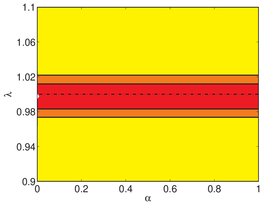
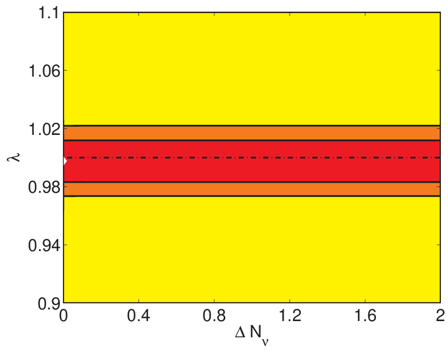
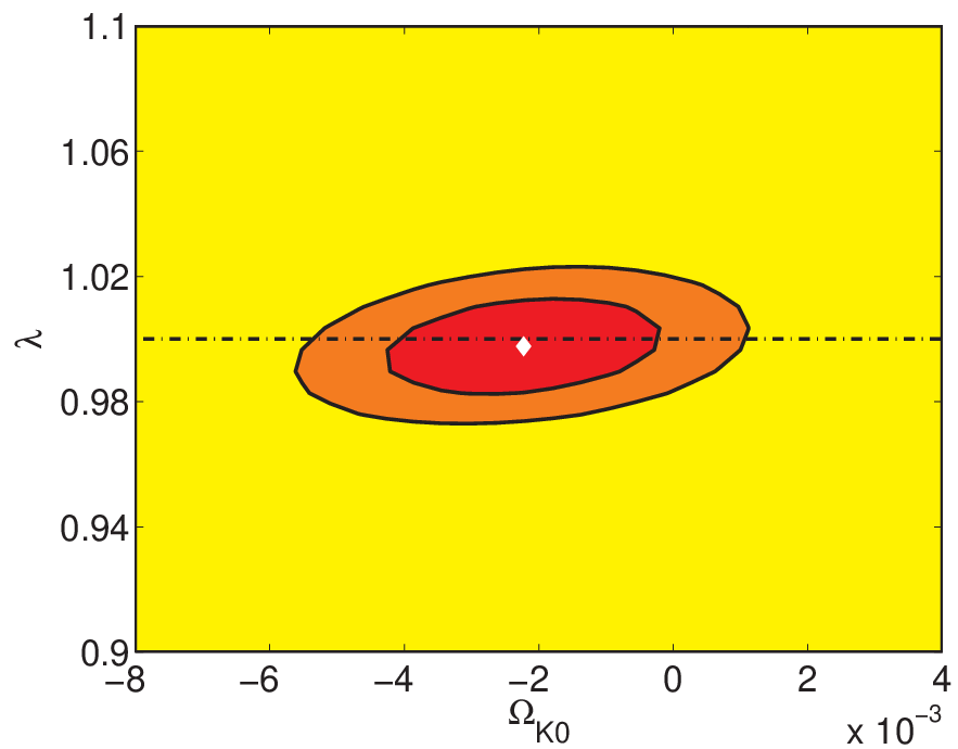
The approximate $1\sigma$ limits on the model parameters $\sigma_{i}$ are presented in Table 2.

Additionally, in Table 3 we focus on the $1\sigma$ limits of $\alpha$ and $\lambda$.

As we observe, in $1\sigma$ confidence the running parameter $\lambda$ of Hořava-Lifshitz gravity is restricted to the interval $|\lambda-1|\lesssim 0.02$, for the entire allowed range of $\omega_{3}$ (that is of $\sigma_{3}$). Finally, the best fit value for $\lambda$ restricts $|\lambda-1|$ to much more smaller values, namely $|\lambda_{b.f}-1|\approx 0.002$.

As can be observed from (25),(26) the action for scalar perturbations includes the two modes $E$ and $\psi$, and their equations of motion read:

As can be seen these two equations are coupled, not allowing for a straightforward stability investigation. However, we can still acquire information about the stability of the configuration by studying it at high and low momenta. Taking the IR limit of (28), that is considering the low-$k$ behavior, it reduces to

Thus, this decoupled equation acts as a low-momentum equation of motion for the scalar field $\psi$. A straightforward observation from (29) is that it leads to a ghost-like behavior, since it leads to the dispersion relation

which induces instabilities, regardless of the $\lambda$-value and of the sign of the cosmological constant. Now, for high $k$, (28) reduces to

Therefore, (31) yields the high-$k$ dispersion relation:

Let us now examine the tensor perturbations. Their action can be extracted from (25),(26) and therefore the graviton equation of motion writes as

Assuming graviton propagation along the $x^{3}$ direction, that is $k_{i}=k^{i}=(0,0,k)$, the $h_{ij}$ can be written as usual in terms of the Left and Right polarization components, and thus we derive the two equations for the different polarizations

where the plus and minus branches correspond to Left-handed and Right-handed modes respectively. In this relation we have identified the light speed from the low $k$ regime as $c^{2}={\kappa^{4}\mu^{2}\Lambda}/[{16(1-3\lambda)}].$ The above equation system accepts a non-trivial solution only if the corresponding determinant is zero, which leads to the dispersion relation

In order to avoid possible accidental artifacts of the detailed-balance condition, in this subsection we extend the investigation beyond detailed balance. As a demonstration, and without loss of generality, we consider a detailed-balance-breaking term of the form $\nabla_{i}R_{jk}\nabla^{i}R^{jk}$. Thus, the corresponding contribution to the action will be [7]

where $\eta$ is an additional parameter. It is straightforward to calculate the modifications that $S^{\left(2\right)}_{bdb}$ brings to the dispersion relations for scalar and tensor perturbations obtained above (expressions (32) and (35) respectively). The extended dispersion relations read:

for scalar perturbations (UV-behavior), and