Minimization of the Probabilistic $p$ -frame Potential

Journal: arXiv.org

M. Ehler Email: ehlermar@mail.nih.gov Corresponding author: Corresponding author Address: National Institutes of Health, National Institute of Child Health and Human Development, Section on Medical Biophysics, Bethesda, MD 20892 Address: University of Maryland, Department of Mathematics, Norbert Wiener Center, College Park, MD 20742 K. A. Okoudjou Email: kasso@math.umd.edu Address: University of Maryland, Department of Mathematics, Norbert Wiener Center, College Park, MD 20742

Abstract

We investigate the optimal configurations of $n$ points on the unit sphere for a class of potential functions. In particular, we characterize these optimal configurations in terms of their approximation properties within frame theory. Furthermore, we consider similar optimal configurations in terms of random distributions of points on the sphere. In this probabilistic setting, we characterize these optimal distributions by means of special classes of probabilistic frames. Our work also indicates some connections between statistical shape analysis and frame theory.

Keywords:

Frame potential, equiangular tight frames, probabilistic frames, directional statistics, statistical shape analysis

2010 MSC

42C15 , 42A61 , 60B05

1 Introduction

Frames are overcomplete (or redundant) sets of vectors that serve to faithfully represent signals. They were introduced in $1952$ by Duffin and Schaeffer [12], and reemerged with the advent of wavelets [9, 11, 15, 18, 21]. Though the overcompleteness of frames precludes signals from having unique representation in the frame expansions, it is, in fact, the driving force behind the use of frames in signal processing [6, 25, 26].

In the finite dimensional setting, frames are exactly spanning sets. However, many applications require “custom-built” frames that possess additional properties which are dictated by these applications. As a result, the construction of frames with prescribed structures has been actively pursued. For instance, a special class called finite unit norm tight frames (FUNTFs) that provide a Parseval-type representation very similar to orthonormal bases, has been customized to model data transmissions [6, 20]. Since then the characterization and construction of FUNTFs and some of their generalizations have received a lot of attention [6, 25, 26]. Beyond their use in applications, FUNTFs are also related to some deep open problems in pure mathematics such as the Kadison-Singer conjecture [7]. FUNTFs appear also in statistics where, for instance, Tyler used them to construct $M$ -estimators of multivariate scatter [32]. We elaborate more on the connection between the $M$ -estimators and FUNTFs in Remark 2.3. These $M$ -estimators were subsequently used to construct maximum likelihood estimators for the the wrapped Cauchy distribution on the circle in [24] and for the angular central Gaussian distribution on the sphere in [33].

FUNTFs are exactly the minimizers of a functional called the frame potential [2]. This was extended to characterize all finite tight frames in [35]. Furthermore, in [19, 22], finite tight frames with a convolutional structure, which can be used to model filter banks, have been characterized as minimizers of an appropriate potential. All these potentials are connected to other functionals whose extremals have long been investigated in various settings. We refer to [10, 13, 29, 34, 36] for details and related results.

In the present paper, we study objects beyond both FUNTFs and the frame potential. In fact, we consider a family of functionals, the $p$ -frame potentials, which are defined on sets $\{x_{i}\}_{i=1}^{N}$ of unit vectors in $\mathbb{R}^{d}$ ; see Section 2. These potentials have been studied in the context of spherical $t$ -designs for even integers $p$ , cf. Seidel in [29], and their minimizers are not just FUNTFs but FUNTFs that inherit additional properties and structure. Common FUNTFs are recovered only for $p=2$ . In the process, we extend Seidel’s results on spherical $t$ -designs in [29] to the entire range of positive real $p$ .

In Section 3, we give lower estimates on the $p$ -frame potentials, and prove that in certain cases their minimizers are FUNTFs, which possess additional properties and structure. In particular, if $0<p\leq 2$ , we completely characterize the minimizers of the $p$ -frame potentials when $N=kd$ for some positive integer $k$ . Moreover, when $N=d+1$ and $0<p\leq 2$ , we characterize the minimizers of the $p$ -frame potentials, under a technical condition, which, we have only been able to establish when $d=2$ . We conjecture that this technical condition holds when $d>2$ . Finally in Section 4, we introduce probabilistic $p$ -frames that generalize the concepts of frames and $p$ -frames. We characterize the minimizers of probabilistic $p$ -frame potentials in terms of probabilistic $p$ -frames. The latter problem is solved completely for $0<p\leq 2$ , and for all even integers $p$ . In particular, these last results generalize [29] as well as the recently introduced notion of the probabilistic frame potential in [16].

Further relations to statistics: Besides the results on FUNTFs used in [24, 32, 33], and mentioned above, frame theory has essentially evolved independently of statistical fields such as statistical shape analysis [14] and directional statistics [27]. Nevertheless, there still exist several overlaps, and to the best of our knowledge, these overlaps have not yet been fully explored. Recently, frame theory has been used in directional statistics [17], where FUNTFs are utilized to investigate on statistical tests for directional uniformity and to model and analyze patterns found in granular rod experiments. We must point out that similar results were obtained earlier by Tyler in [33].

Probabilistic tight frames are multivariate probability distributions whose second moments’ matrix is a multiple of the identity, and they are used in [16] to obtain approximate FUNTFs. The latter approximation procedure is connected to a classical problem in multivariate statistics, namely estimating the population covariance from a sample, which is closely related to the $M$ -estimators addressed in [24, 32, 33]. The $p$ -frame potentials and their probabilistic counterparts that we consider in the sequel, are linked to the notion of shape measure, shape space, and mean shape used in statistical shape analysis. In Section 2.2, we establish a precise connection between the full Procrustes estimate of mean shape [23, Definition 3.3] which is the eigenvector corresponding to the largest eigenvalue of the frame operator. Moreover, this eigenvalue coincides with the upper frame redundancy as introduced in [4]. The full Procrustes estimate of mean shape also saturates the upper frame inequality. Moreover, the $p$ -frame potentials form size measures as required in statistical shape analysis, and their minimizers among all collections of $N$ points on the sphere define a shape space modulo rotations.

We hope that the present paper will renew interests in more investigation on the role of frames and the $p$ -th frame potential in directional statistics and statistical shape analysis.

2 The $p$ -frame potential

2.1 Background on frames and the frame potential

To introduce frames and their elementary properties, we follow the textbook [8].

Definition 2.1.

A collection of points $\{x_{i}\}_{i=1}^{N}\subset\mathbb{R}^{d}$ is called a finite frame for $\mathbb{R}^{d}$ if there are two constants $0<A\leq B$ such that

A\|x\|^{2}\leq\sum_{i=1}^{N}|\langle x,x_{i}\rangle|^{2}\leq B\|x\|^{2},\quad\text{for all $x\in\mathbb{R}^{d}$.}

(1)

If the frame bounds $A$ and $B$ are equal, the frame $\{x_{i}\}_{i=1}^{N}\subset\mathbb{R}^{d}$ is called a finite tight frame for $\mathbb{R}^{d}$ . In this case,

A\|x\|^{2}=\sum_{i=1}^{N}|\langle x,x_{i}\rangle|^{2},\quad\text{for all $x\in\mathbb{R}^{d}$.}

(2)

A finite tight frame $\{x_{i}\}_{i=1}^{N}\subset\mathbb{R}^{d}$ consisting of unit norm vectors is called a finite unit norm tight frame (FUNTF) for $\mathbb{R}^{d}$ . In this case, the frame bound is $A=N/d$ .

A collection of unit vectors $\{x_{i}\}_{i=1}^{N}\subset S^{d-1}$ is called equiangular if there exists a nonnegative constant $C$ such that $|\langle x_{i},x_{j}\rangle|=C$ , for $i\neq j$ .

Given a collection of $N$ points $\{x_{i}\}_{i=1}^{N}$ in $\mathbb{R}^{d}$ , the analysis operator is the mapping

F:\mathbb{R}^{d}\rightarrow\mathbb{R}^{N},\quad x\mapsto\big(\langle x,x_{i}\rangle\big)_{i=1}^{N}.

Its adjoint operator is called the synthesis operator and given by

F^{*}:\mathbb{R}^{N}\rightarrow\mathbb{R}^{d},\quad(c_{i})_{i=1}^{N}\mapsto\sum_{i=1}^{N}c_{i}x_{i}.

Using these operators, it is easy to see that $\{x_{i}\}_{i=1}^{N}$ is a frame if and only if the frame operator defined by

S:=F^{*}F:\mathbb{R}^{d}\rightarrow\mathbb{R}^{d},\quad x\mapsto\sum_{i=1}^{N}\langle x,x_{i}\rangle x_{i}

is positive, self-adjoint, and invertible. In this case, the following reconstruction formula holds

x=\sum_{j=1}^{N}\langle S^{-1}x_{i},x\rangle x_{i},\text{ for all $x\in\mathbb{R}^{d}$,}

(3)

and $\{S^{-1}x_{i}\}_{i=1}^{N}$ , in fact, is a frame too, called the canonical dual frame. If $\{x_{i}\}_{i=1}^{N}$ is a frame, then $\{S^{-1/2}x_{i}\}_{i=1}^{N}$ is a finite tight frame. Moreover, note that $\{x_{i}\}_{i=1}^{N}$ is a FUNTF if and only if its frame operator $S$ is $\frac{N}{d}$ times the identity.

As mentioned in the introduction, the question of the existence and characterization of FUNTFs was settled in [2], where the frame potential, defined by

\FP(\{x_{i}\}_{i=1}^{N})=\sum_{i=1}^{N}\sum_{j=1}^{N}|\langle x_{i},x_{j}\rangle|^{2},

(4)

was introduced and used to give a characterization of its minimizers in terms of FUNTFs. More specifically, they prove the following result:

Theorem 2.2.

[2, Theorem 7.1] Let $N$ be fixed and consider the minimization of the frame potential among all collections of $N$ points on the sphere $S^{d-1}$ .

a)

If $N\leq d$ , then the minimum of the frame potential is $N$ . The minimizers are exactly the orthonormal systems for $\mathbb{R}^{d}$ with $N$ elements.
b)

If $N\geq d$ , then the minimum of the frame potential is $\frac{N^{2}}{d}$ . The minimizers are exactly the FUNTFs for $\mathbb{R}^{d}$ with $N$ elements.

We shall prove in the sequel that the frame potential is just an example in a family of functionals defined on points on the sphere, and whose minimizers have approximation properties similar to those of the frame potential. But first, we briefly comment on the relation between FUNTFs and $M$ -estimators of multivariate scatter:

Remark 2.3.

The concept of FUNTFs is used in signal processing to represent a signal $x\in\mathbb{R}^{d}$ by means of $x=\frac{d}{N}\sum_{i=1}^{N}\langle x,x_{i}\rangle x_{i}$ , which is similar to the well-known expansion in an orthonormal basis. FUNTFs have also been used in statistics to derive $M$ -estimators of multivariate scatter: For a sample $\{x_{i}\}_{i=1}^{N}\subset\mathbb{R}^{d}$ , where $x_{i}\neq 0$ , for $i=1\ldots,N$ , Tyler aims to find a symmetric positive definite matrix $\Gamma$ such that

M(\Gamma)=\frac{d}{N}\sum_{i=1}^{N}\frac{\Gamma^{1/2}x_{i}x_{i}^{\prime}\Gamma^{1/2}}{x_{i}^{\prime}\Gamma x_{i}}

is the identity matrix. Whenever this is possible, the estimate $V$ of the population scatter matrix is then given by $V=\Gamma^{-1}$ . We refer to [32] for details. Note that $M(\Gamma)=I_{d}$ implies that

\bigg\{\frac{\Gamma^{1/2}x_{i}}{\sqrt{x_{i}^{\prime}\Gamma x_{i}}}\bigg\}_{i=1}^{N}=\bigg\{\frac{\Gamma^{1/2}x_{i}}{\|\Gamma^{1/2}x_{i}\|}\bigg\}_{i=1}^{N}\subset S^{d-1}

forms a FUNTF. Moreover, $\{x_{i}\}_{i=1}^{N}\subset S^{d-1}$ is a FUNTF if and only if $M(I_{d})=I_{d}$ .

2.2 Definition of the $p$ -frame potential

Definition 2.4.

Let $N$ be a positive integer, and $0<p<\infty$ . Given a collection of unit vectors $\{x_{i}\}_{i=1}^{N}\subset S^{d-1}$ , the $p$ -frame potential is the functional

\FP_{p,N}(\{x_{i}\}_{i=1}^{N})=\sum_{i,j=1}^{N}|\langle x_{i},x_{j}\rangle|^{p}.

(5)

When, $p=\infty$ , the definition reduces to

\FP_{\infty,N}(\{x_{i}\}_{i=1}^{N})=\sup_{i\neq j}|\langle x_{i},x_{j}\rangle|.

It is clear that the $p$ -frame potential generalizes the frame potential in (4). Finite frames and the $p$ -frame potential also extend to complex $\{z_{i}\}_{i=1}^{N}\subset S_{\mathbb{C}}^{d-1}=\{z\in\mathbb{C}^{d}:\|z\|=1\}$ and are related to statistical shape analysis, a tool to quantitatively track the physical deformation of objects. We refer to [14, Chapters 2, 3 $\&$ 4] for more details on shape analysis, but we briefly indicate here its link to the $p$ -frame potential. The shape of an object is specified by landmark points that altogether form the shape space. Often, a suitable transformation is applied first in order to study shape independently on the object’s size. To remove the feature of size, we must specify a size measure $g$ ([14, Definition 2.2]), which is a positive function defined on $S_{\mathbb{C}}^{d-1}$ that satisfies

g(s\{z_{i}\}_{i=1}^{N})=sg(\{z_{i}\}_{i=1}^{N}),\quad\text{for all $s\in\mathbb{R}_{+}$ and $\{z_{i}\}_{i=1}^{N}\subset S_{\mathbb{C}}^{d-1}$}.

It is immediate that the following family of functionals can be seen as size measures:

g_{p}(\{z_{i}\}_{i=1}^{N}):=\big(\sum_{i,j=1}^{N}|\langle z_{i},z_{j}\rangle|^{p}\big)^{\frac{1}{p}}=\bigg(\FP_{N,p}(\{z_{i}\}_{i=1}^{N})\bigg)^{1/p}.

In particular, $g_{1}$ represents the centroid size (when the shape is centered at the origin), which is one of the most common size measures in statistical shape analysis. Given two complex configurations $z_{1},z_{2}\in\mathbb{C}^{d}$ derived from landmarks that code two-dimensional shape, the full Procrustes distance ([14, Definition 3.2]) is

d_{F}(z_{1},z_{2})=\inf_{\beta,\theta,a,b}\bigg\|\frac{z_{1}}{\|z_{1}\|}-\frac{z_{2}}{\|z_{2}\|}\beta e^{i\theta}-a-ib\bigg\|.

Given $N$ configurations $\{z_{i}\}_{i=1}^{N}\subset\mathbb{C}^{d}$ , the full Procrustes estimate of mean shape is defined by

\bar{z}_{P}=\arg\inf_{\|z\|=1}\big(\sum_{i=1}^{N}d_{F}^{2}(z_{i},z)\big),

cf. [14, Definition 3.3]. The average axis from the complex Bingham maximum likelihood estimator is the same as the full Procrustes estimate of mean shape for two-dimensional shapes, and the same holds for the complex Watson distribution, cf. [14, Sections 6.2 $\&$ 6.3]. If we assume that $\{z_{i}\}_{i=1}^{N}$ are centered around zero, then $\bar{z}_{P}$ is given by the eigenvector corresponding to the largest eigenvalue $\lambda$ of the frame operator of the normalized collection $\{\frac{z_{i}}{\|z_{i}\|}\}_{i=1}^{N}$ . Furthermore, one observes that this eigenvalue $\lambda$ is the upper frame redundancy of $\{z_{i}\}_{i=1}^{N}$ as introduced in [4], which also coincides with the optimal upper frame bound $B$ in (1). Therefore, the full Procrustes estimate of mean shape satisfies the upper frame inequality with equality. Moreover, we have observed that the root mean square of the full Procrustes estimate of mean shape is $1-\frac{\lambda}{N}$ .

Before stating the next elementary result, we recall some basic definitions in physics: A conservative force $F$ , is a vector field defined on $\mathbb{R}^{d}$ , such that $-F$ is the gradient of some potential $P$ that is then induced by the conservative force. Lemma 2.5 below was proved for the frame potential in [2], and we extend it to all $p$ -frame potentials with $1<p<\infty$ :

Lemma 2.5.

For each $p\in(1,\infty)$ , the $p$ -frame potential $\FP_{p,N}$ is induced by the conservative force $F_{p}=f_{p}(\|a-b\|)(a-b)$ , for $a,b\in S^{d-1}$ , where

f_{p}(x):=\begin{cases}p(1-\frac{x^{2}}{2})^{p-1},&\text{for }|x|\leq\sqrt{2},\\ -p(\frac{x^{2}}{2}-1)^{p-1},&\text{otherwise.}\end{cases}

$F_{p}$ is a central force between the ‘particles’ $a$ and $b$ that we call the $p$ -frame force.

Proof.

The function

\mathbf{p}_{p}(x):=|1-\frac{x^{2}}{2}|^{p}=\begin{cases}(1-\frac{x^{2}}{2})^{p},&\text{for }|x|\leq\sqrt{2},\\ (\frac{x^{2}}{2}-1)^{p},&\text{otherwise,}\end{cases}

is differentiable and satisfies $\mathbf{p}_{p}^{\prime}(x)=-xf_{p}(x)$ . This is sufficient to verify that the potential $P_{p}(a,b):=\mathbf{p}_{p}(\|a-b\|)$ , defined for $a,b\in S^{d-1}$ , satisfies $\nabla_{a}P_{p}(a,b)=-F(a,b)$ , where $b$ is held fixed. Thus, $F_{p}$ is a conservative vector field. The physical meaningful potential $P_{p}(a,b)$ is in fact given by

P_{p}(a,b)=\mathbf{p}_{p}(\|a-b\|)=\big|1-\frac{1}{2}\|a-b\|^{2}\big|^{p}=\big|\langle a,b\rangle\big|^{p},

where we used that $\|a\|=\|b\|=1$ . Consequently, the $p$ -frame potential is induced by the conservative central force $F_{p}$ . ∎

As a consequence of the above lemma, $\{x_{i}\}_{i=1}^{N}\subset S^{d-1}$ are in equilibrium under the $p$ -frame force if they minimize the $p$ -frame potential among all collections of $N$ points on the sphere. Note that such a collection of equilibria modulo rotations form a shape space.

Remark 2.6.

We will use repeatedly the fact that for a fixed $\{x_{i}\}_{i=1}^{N}\subset S^{d-1}$ , the $p$ -frame potential $\FP_{p,N}(\{x_{i}\}_{i=1}^{N})$ is a decreasing and continuous function of $p\in(0,\infty)$ .

3 Lower estimates for the $p$ -frame potential

We start this section with a few elementary results about the minimizers of the $p$ -frame potential as well as their connection to $t$ -designs. In fact, potentials on the sphere, and $t$ -designs have been well investigated [1, 10, 13, 29, 34]. However, one of the key differences between $t$ -designs and our $p$ -frame potential is that the former is considered only for positive integers $t$ while the latter is investigated for $p\in(0,\infty)$ .

3.1 The Welch bound revisited

If $p=2k$ is an even integer, one can use Welch’s results [36] to conclude that, for $\{x_{i}\}_{i=1}^{N}\subset S^{d-1}$ ,

\FP_{p,N}(\{x_{i}\}_{i=1}^{N})\geq\frac{N^{2}}{\binom{d+k-1}{k}}.

(6)

We shall verify that this estimate is not optimal for small $N$ , by proving an estimate for $\FP_{p,N}$ when $2<p<\infty$ . The following Proposition first appeared in [28]:

Proposition 3.1.

Let $\{x_{i}\}_{i=1}^{N}\subset S^{d-1}$ , $N\geq d$ , and $2<p<\infty$ , then

\FP_{p,N}(\{x_{i}\}_{i=1}^{N})\geq N(N-1)\big(\frac{N-d}{d(N-1)}\big)^{p/2}+N,

(7)

and equality holds if and only if $\{x_{i}\}_{i=1}^{N}$ is an equiangular FUNTF.

Proof.

For $\frac{1}{2}=\frac{1}{p}+\frac{1}{r}$ , Hölder’s inequality yields

\|(\langle x_{i},x_{j}\rangle)_{i\neq j}\|_{\ell_{2}}\leq\|(\langle x_{i},x_{j}\rangle)_{i\neq j}\|_{\ell_{p}}(N(N-1))^{1/r}.

(8)

Raising to the $p$ -th power and applying $\frac{1}{r}=\frac{1}{2}-\frac{1}{p}$ leads to

\|(\langle x_{i},x_{j}\rangle)_{i\neq j}\|_{\ell_{2}}^{p}\leq\|(\langle x_{i},x_{j}\rangle)_{i\neq j}\|_{\ell_{p}}^{p}(N(N-1))^{p/2-1}.

(9)

Therefore,

\sum_{i\neq j}|\langle x_{i},x_{j}\rangle|^{p}\geq\big(\sum_{i\neq j}|\langle x_{i},x_{j}\rangle|^{2}\big)^{p/2}(N(N-1))^{1-p/2}.

Using the fact that $\sum_{i\neq j}|\langle x_{i},x_{j}\rangle|^{2}\geq\frac{N^{2}}{d}-N$ (see Theorem 2.2) implies that

\sum_{i\neq j}|\langle x_{i},x_{j}\rangle|^{p}\geq\big(N(\frac{N}{d}-1)\big)^{p/2}(N(N-1))^{1-p/2}=N(N-1)\bigg(\frac{N-d}{d(N-1)}\bigg)^{p/2},

which proves (7).

To establish the last part of the Proposition, we recall that an equiangular FUNTF $\{x_{k}\}_{k=1}^{N}\subset\mathbb{R}^{d}$ satisfies

|\langle x_{i},x_{j}\rangle|=\sqrt{\frac{N-d}{d(N-1)}},\quad\text{ for all }i\neq j

(10)

see, [5, 31], for details. Consequently, if $\{x_{k}\}_{k=1}^{N}$ is an equiangular FUNTF, then (7) holds with equality.

On the other hand, if equality holds in (7), then $\sum_{i\neq j}|\langle x_{i},x_{j}\rangle|^{2}=\frac{N^{2}}{d}-N$ and $\{x_{i}\}_{i=1}^{N}$ is a FUNTF due to Theorem 2.2. Moreover, the Hölder estimate (8) must have been an equality which means that $|\langle x_{i},x_{j}\rangle|=C$ for $i\neq j$ , and some constant $C\geq 0$ . Thus, the FUNTF must be equiangular. ∎

By comparing (6) with (7), it is easily seen that the Welch bound is not optimal for small $N$ :

Proposition 3.2.

Let $\{x_{i}\}_{i=1}^{N}\subset S^{d-1}$ and $p=2k>2$ be an even integer. If $d<N\leq\binom{d+k-1}{k}$ , then

\FP_{p,N}(\{x_{k}\}_{k=1}^{N})\geq N(N-1)\big(\frac{N-d}{d(N-1)}\big)^{k}+N>\frac{N^{2}}{\binom{d+k-1}{k}}.

(11)

Proof.

The condition on $N$ implies $1\geq\frac{N}{\binom{d+k-1}{k}}$ , and adding $(N-1)\big(\frac{N-d}{d(N-1)}\big)^{k}>0$ to the right hand side leads to

(N-1)\big(\frac{N-d}{d(N-1)}\big)^{k}+1>\frac{N}{\binom{d+k-1}{k}}.

Multiplication by $N$ and Proposition 3.1 then yield (11). ∎

Remark 3.3.

The estimate in Proposition 3.1 is sharp if and only if an equiangular FUNTF exists. In [31, Sections 4 $\&$ 6], construction (and hence existence) of equiangular FUNTFs was established when $d+2\leq N\leq 100$ . For general $d$ and $N$ , a necessary condition for existence of equiangular FUNTFs is given, and it is conjectured that the conditions are sufficient as well. The authors essentially provide on upper bound on $N$ that depends on the dimension $d$ . Therefore, Proposition 3.1 might not be optimal when the redundancy $N/d$ is much larger than $1$ .

3.2 Relations to spherical $t$ -designs

A spherical $t$ -design is a finite subset $\{x_{i}\}_{i=1}^{N}$ of the unit sphere $S^{d-1}$ in $\mathbb{R}^{d}$ , such that,

\frac{1}{N}\sum_{i=1}^{N}h(x_{i})=\int_{S^{d-1}}h(x)d\sigma(x),

for all homogeneous polynomials $h$ of total degree equals or less than $t$ in $d$ variables and where $\sigma$ denotes the uniform surface measure on $S^{d-1}$ normalized to have mass one. The following result is due to [34, Theorem 8.1] (see [29], [13] for similar results).

Theorem 3.4.

[34, Theorem 8.1] Let $p=2k$ be an even integer and $\{x_{i}\}_{i=1}^{N}=\{-x_{i}\}_{i=1}^{N}\subset S^{d-1}$ , then

\FP_{p,N}(\{x_{i}\}_{i=1}^{N})\geq\frac{1\cdot 3\cdot 5\cdots(p-1)}{d(d+2)\cdots(d+p-2)}N^{2},

and equality holds if and only if $\{x_{i}\}_{i=1}^{N}$ is a spherical $p$ -design.

3.3 Optimal configurations for the $p$ -frame potential

We first use Theorem 2.2 to characterize the minimizers of the $p$ -frame potential for $0<p<2$ provided that the number of points $N$ is a multiple of the dimension $d$ :

Theorem 3.5.

Let $0<p<2$ and assume that $N=kd$ for some positive integer $k$ . Then the minimizers of the $p$ -frame potential are exactly the $k$ copies of any orthonormal basis modulo multiplications by $\pm 1$ . The minimum of (5), over all sets of $N=kd$ unit norm vectors, is $k^{2}d$ .

Proof.

If we fix a collection of vectors $\{x_{i}\}_{i=1}^{N}$ , then the frame potential is a decreasing function in $p\in(0,2)$ . Therefore,

N^{2}/d=\FP_{2,N}(\{x_{i}\}_{i=1}^{N})\leq\FP_{p,N}(\{x_{i}\}_{i=1}^{N}).

Now suppose that $\{y_{i}\}_{i=1}^{N}$ consists of $k$ copies of an orthonormal basis $\{e_{i}\}_{i=1}^{d}$ for $\mathbb{R}^{d}$ . Then,

\min\FP_{p,N}(\{x_{i}\}_{i=1}^{N})\leq\FP_{p,N}(\{y_{i}\}_{i=1}^{N})=\FP(\{y_{i}\}_{i=1}^{N})=N^{2}/d.

Consequently,

\min\FP_{p,N}(\{x_{k}\}_{k=1}^{N})=\min\FP(\{x_{k}\}_{k=1}^{N})=N^{2}/d.

Thus, $\FP_{p,N}$ has the same minimum as $\FP$ . Clearly $k$ copies of an orthonormal basis of $\mathbb{R}^{d}$ form a FUNTF, and hence minimize the $\FP$ due to Theorem 2.2. Consequently, the $k$ copies of an orthonormal basis also minimize the $p$ -frame potential for $0<p<2$ . On the other hand, the inner products must be $0$ or $1$ to obtain a minimizer. The smallest $p$ -frame potential then have the $k$ copies of an orthonormal basis. ∎

We now consider the $p$ -frame potential for $N=d+1$ . The case $p=2$ is covered by Theorem 2.2. Note that any FUNTF with $N=d+1$ vectors is equiangular [20, 30]. Hence, the case $2<p<\infty$ is settled by Proposition 3.1, so we focus on $p\in(0,2)$ .

One easily verifies that, for $p_{0}=\frac{\log(\frac{d(d+1)}{2})}{\log(d)}$ , an orthonormal basis plus one repeated vector and an equiangular FUNTF have the same $p_{0}$ -frame potential $\FP_{p_{0},d+1}$ . Under the assumption that those two systems are exactly the minimizers of $\FP_{p_{0},d+1}$ , the next result will give a complete characterization of the minimizers of $\FP_{p,d+1}$ , for $0<p<2$ . However, we have only been able to establish the validity of this assumption when $d=2$ , cf. Corollary 3.7.

Theorem 3.6.

Let $N=d+1$ and set $p_{0}=\frac{\log(\frac{d(d+1)}{2})}{\log(d)}=\frac{\log(\frac{N(N-1)}{2})}{\log(N-1)}$ . Let $\{x_{i}\}_{i=1}^{N}\subset S^{d-1}$ , and assume that $\FP_{p_{0},N}(\{x_{i}\}_{i=1}^{N})\geq N+2,$ with equality holds if and only if $\{x_{i}\}_{i=1}^{N}$ is an orthonormal basis plus one repeated vector or an equiangular FUNTF. Then,

(1)

for $0<p<p_{0}$ , then for any $\{x_{i}\}_{i=1}^{N}\subset S^{d-1}$ , we have $\FP_{p,N}(\{x_{i}\}_{i=1}^{N})\geq N+2,$ and equality holds if and only if $\{x_{i}\}_{i=1}^{N}$ is an orthonormal basis plus one repeated vector,
(2)

for $p_{0}<p<2$ , then for any $\{x_{i}\}_{i=1}^{N}\subset S^{d-1}$ , we have $\FP_{p,N}(\{x_{i}\}_{i=1}^{N})\geq 2^{\frac{p}{p_{0}}}\,(Nd)^{1-\frac{p}{p_{0}}}+N,$ and equality holds if and only if $\{x_{i}\}_{i=1}^{N}$ is an equiangular FUNTF.

Proof.

Under the assumptions of the Theorem, let $0<p<p_{0}$ , then

\min\FP_{p_{0},N}(\{x_{i}\}_{i=1}^{N})\leq\min\FP_{p,N}(\{x_{i}\}_{i=1}^{N}),

and using $\{y_{i}\}_{i=1}^{N}$ consisting of an orthonormal basis of $\mathbb{R}^{d}$ with one repeated vector, yields that

\min\FP_{p,N}(\{x_{i}\}_{i=1}^{N})\leq\FP_{p,N}(\{y_{i}\}_{i=1}^{N})=N+2=\min\FP_{p_{0},N}(\{x_{i}\}_{i=1}^{N}).

Consequently, $\min\FP_{p_{0},N}(\{x_{i}\}_{i=1}^{N})=\min\FP_{p,N}(\{x_{i}\}_{i=1}^{N})=N+2$ . Since an orthonormal basis plus one repeated vector minimizes the $p$ -frame potential for $p=p_{0}$ , it must also minimize $\FP_{p,N}$ for $0<p<p_{0}$ , which proves $(1)$ .

Assume now that $p_{0}<p<2$ . Choose $r$ such that $\frac{1}{p_{0}}=\frac{1}{p}+\frac{1}{r}$ , Hölder’s inequality yields

\|(\langle x_{i},x_{j}\rangle)_{i\neq j}\|_{\ell_{p_{0}}}^{p}\leq\|(\langle x_{i},x_{j}\rangle)_{i\neq j}\|_{\ell_{p}}^{p}(N^{2}-N)^{p/r}.

Since we assume that $(2)$ holds, we have $\sum_{i\neq j}|\langle x_{i},x_{j}\rangle|^{p_{0}}\geq 2$ , which leads to

	$\displaystyle\sum_{i\neq j}\|\langle x_{i},x_{j}\rangle\|^{p}$	$\displaystyle\geq\bigg(\sum_{i\neq j}\|\langle x_{i},x_{j}\rangle\|^{p_{0}}\bigg){\frac{p}{p_{0}}}(N^{2}-N)^{1-\frac{p}{p_{0}}}$
		$\displaystyle\geq 2^{\frac{p}{p_{0}}}\,(Nd)^{1-\tfrac{p}{p_{0}}}.$

This concludes the proof of $(2)$ . By applying (10), one then checks that an equiangular FUNTF satisfies $(2)$ with equality.

The “only” part comes from the fact that the Hölder inequality becomes an equality only if the sequences are linearly dependent. This means that the $\{x_{i}\}_{i=1}^{N}$ are equiangular. They must then satisfy $|\langle x_{i},x_{j}\rangle|=\frac{1}{d}$ . Thus, by (10) they form an equiangular FUNTF [5, 31]. ∎

When $d=2$ we can in fact verify the main hypothesis of Theorem 3.6, which leads to the following result:

Corollary 3.7.

Let $\{x_{i}\}_{i=1}^{3}\subset S^{1}$ , and set $p_{0}=\frac{\log(3)}{\log(2)}$ . Then,

\FP_{p_{0},3}(\{x_{i}\}_{i=1}^{3})\geq 5,

and equality holds if and only if $\{x_{i}\}_{i=1}^{3}$ is an orthonormal basis plus one repeated vector or an equiangular FUNTF.

Consequently,

(1)

for $0<p<p_{0}$ , then for any $\{x_{i}\}_{i=1}^{3}\subset S^{1}$ , we have $\FP_{p,3}(\{x_{i}\}_{i=1}^{3})\geq 5,$ and equality holds if and only if $\{x_{i}\}_{i=1}^{3}$ is an orthonormal basis plus one repeated vector,
(2)

for $p_{0}<p<\infty$ , then for any $\{x_{i}\}_{i=1}^{3}\subset S^{1}$ , we have $\FP_{p,3}(\{x_{i}\}_{i=1}^{3})\geq\frac{6}{2^{p}}+3,$ and equality holds if and only if $\{x_{i}\}_{i=1}^{3}$ is an equiangular FUNTF.

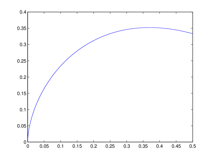
The minimum of $\FP_{p,3}$ , for $0<p<\infty$ is plotted in Figure 1.

Refer to caption — Figure 1: Minimum of $\FP_{p,3}$ in Corollary 3.7, for $0<p<10$ .

Proof.

Clearly $(1)$ and $(2)$ follows from Theorem 3.6 once the minimizers of $\FP_{p_{0},N}$ are characterized.

Without loss of generality, let $\beta$ be the smallest angle between $x_{1}$ , $x_{2}$ , and $x_{3}$ and let $\alpha$ be the second smallest angle between them. This yields, of course, $0\leq\beta\leq\alpha$ .

Case 1: For $0\leq\alpha+\beta\leq\frac{\pi}{2}$ , we have

\frac{1}{2}\sum_{i\neq j}|\langle x_{i},x_{j}\rangle|^{p}=\cos^{p}(\alpha)+\cos^{p}(\beta)+\cos^{p}(\alpha+\beta)=F(\alpha,\beta).

Since $1<p_{0}$ , the $p$ -frame potential is differentiable in $\alpha$ and $\beta$ , and its critical points are

	$\displaystyle 0$	$\displaystyle=-p\cos^{p-1}(\alpha)\sin(\alpha)-p\cos^{p-1}(\alpha+\beta)\sin(\alpha+\beta)$
	$\displaystyle 0$	$\displaystyle=-p\cos^{p-1}(\beta)\sin(\beta)-p\cos^{p-1}(\alpha+\beta)\sin(\alpha+\beta).$

This implies that either $\alpha=\beta=0$ or $\beta=0$ and $\alpha=\frac{\pi}{2}$ . In the first case, we have a maximum since it implies $x_{1}=x_{2}=x_{3}$ . The latter case means that two points are identical and the third one is perpendicular which is a potential minimum of the $p$ -frame potential.

Case 2: We can assume that $\frac{\pi}{4}\leq\alpha$ (otherwise we are in Case 1). We can further assume that $\frac{\pi}{4}\leq\alpha\leq\frac{\pi}{2}\leq\alpha+\beta\leq\frac{2\pi}{3}$ (if $\frac{2\pi}{3}<\alpha+\beta\leq\pi$ . Otherwise, substitute $x_{i}$ with $-x_{i}$ . We now have

\frac{1}{2}\sum_{i\neq j}|\langle x_{i},x_{j}\rangle|^{p}=\cos^{p}(\alpha)+\cos^{p}(\beta)+(-\cos(\alpha+\beta))^{p}=G(\alpha,\beta).

The critical points of $G$ are given by

	$\displaystyle 0$	$\displaystyle=-p\cos^{p-1}(\alpha)\sin(\alpha)+p(-\cos(\alpha+\beta))^{p-1}\sin(\alpha+\beta)$
	$\displaystyle 0$	$\displaystyle=-p\cos^{p-1}(\beta)\sin(\beta)+p(-\cos(\alpha+\beta))^{p-1}\sin(\alpha+\beta).$

By subtracting one equation from the other and raising to the second power, we obtain

z_{1}^{p-1}(1-z_{1})=z_{2}^{p-1}(1-z_{2}),

where $z_{1}=\cos(\alpha)^{2}$ and $z_{2}=\cos^{2}(\alpha+\beta)$ . Since $\sin^{2}(x)-1/2\geq\cos^{2}(x)$ for all $\pi/2\leq x\leq 2\pi/3$ , we have $0\leq z_{1}\leq 1/2$ and $0\leq z_{2}\leq 1/4$ because $z_{2}\leq 1-z_{2}-1/2$ .

We consider the function $F(z)=z^{p-1}(1-z)$ on $0\leq z\leq 1/2$ . $F$ achieves its maximum at $z=\frac{p-1}{p}\approx 0.3691$ and is convex, cf. Figure 2.

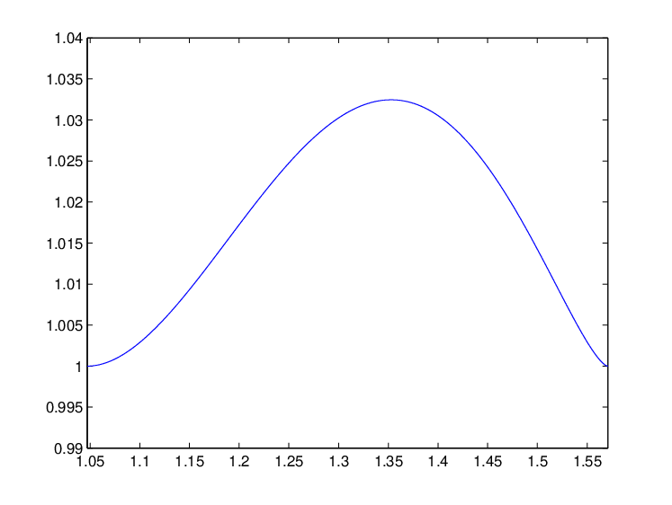
Therefore, for $0\leq z_{1}\leq 1/2$ and $0\leq z_{2}\leq 1/4$ , we have $F(z_{1})=F(z_{2})$ if and only if $z_{1}=z_{2}$ or $z_{1}=1/2$ and $z_{2}=1/4$ . For $z_{1}=\cos^{2}(\alpha)=1/2$ , we have $\alpha=\pi/3$ and $z_{2}=\cos^{2}(\pi/3+\beta)=1/4$ yields $\beta=\pi/3$ . The case $z_{1}=z_{2}$ leads to $\cos^{2}(\alpha)=\cos^{2}(\alpha+\beta)$ which implies $\alpha+\beta-\pi/2=\pi/2-\alpha$ . This is equivalent to $\beta=\pi-2\alpha$ . Since we assume $\beta\leq\alpha$ , we obtain $\pi/3\leq\alpha\leq\pi/2$ .

We now check the minima of the function

	$\displaystyle f(\alpha)$	$\displaystyle=\cos^{p}(\alpha)+\cos^{p}(\pi-2\alpha)+(-\cos(\pi-\alpha))^{p}$
		$\displaystyle=2\cos^{p}(\alpha)+(-\cos(2\alpha))^{p},$

on $\pi/3\leq\alpha\leq\pi/2$ , cf. Figure 2. Its derivative

\frac{\partial f}{\partial\alpha}(\alpha)=-2p\cos^{p-1}(\alpha)\sin(\alpha)+2p(-\cos(2\alpha))^{p-1}\sin(2\alpha)

vanishes if and only if

\cos^{p-1}(\alpha)\sin(\alpha)=(\sin^{2}(\alpha)-\cos^{2}(\alpha))^{p-1}2\cos(\alpha)\sin(\alpha)

For $\alpha\neq\pi/2$ , this yields

\cos^{p-1}(\alpha)=(1-2\cos^{2}(\alpha))^{p-1}2\cos(\alpha).

By substituting $x=\cos(\alpha)$ , we obtain, for $0<x\leq 1/2$

x^{p-1}=(1-2x^{2})^{p-1}2x,

which is equivalent to

1/2=(1/x-2x)^{p-1}x\Leftrightarrow 0=(1/x-2x)x^{1/(p-1)}-(1/2)^{1/(p-1)}

and define the new function

g(x)=-2x^{q+1}+x^{q-1}-(1/2)^{q},

where $q=1/(p-1)$ . To show that $g$ has only one extremal point on $0<x\leq 1/2$ , we differentiate

\frac{\partial g}{\partial x}(x)=-2(q+1)x^{q}+(q-1)x^{q-2}.

The term $\frac{\partial g}{\partial x}(x)$ vanishes if and only if

(q-1)x^{q-2}=2(q+1)x^{q},

which is equivalent to

x^{2}=\frac{q-1}{2(q+1)}=\frac{2-\log_{2}(3)}{2\log_{2}(3)}.

Hence, $x\approx 0.3618$ and $\frac{\partial g}{\partial x}$ does not have any other zeros on $0<x\leq 1/2$ . This means that $g$ has only one extremal point and can then only have two zeros on $0<x\leq 1/2$ . The zero at $x=1/2$ corresponds to a minimum. This means that the zero of $\frac{\partial g}{\partial x}$ at $x\approx 0.3618$ is a maximum of $g$ . Hence the other zero of g is between $0$ and $\approx 0.3618$ . However, this other zero corresponds to a maximum of $f$ . The minimum of $f$ can thus be at $x=0$ or $x=1/2$ . This implies $\alpha=\pi/3$ or $\alpha=\pi/2$ . It is easy to verify that $\alpha=\pi/3$ would lead to $\beta=\pi/3$ , and $\alpha=\pi/2$ yields $\beta=0$ . Thus, the minimum of the $p$ -frame potential corresponds to either an orthonormal basis plus one repeated element ( $\alpha=\pi/2$ , $\beta=0$ ) or an equiangular FUNTF ( $\alpha=\beta=\pi/3$ ). One easily checks that both situations lead to the same global minimum.

∎

In view of Theorem 3.6 and Corollary 3.7, we have the following conjecture:

Conjecture 3.8.

Let $N=d+1$ and $p_{0}=\frac{\log(\frac{d(d+1)}{2})}{\log(d)}$ . Then

\FP_{p_{0},N}(\{x_{k}\}_{k=1}^{N})\geq N+2,

and equality holds if and only if $\{x_{i}\}_{i=1}^{N}$ is an orthonormal basis plus one repeated vector or an equiangular FUNTF.

One can check that $1<p_{0}<2$ , for $d>1$ . According to Proposition 3.1, the minimizers of the $p$ -frame potential for $2<p<\infty$ are exactly the equiangular FUNTFs. Thus, our conjecture essentially addresses the range $0<p<2$ .

Remark 3.9.

Although we are primarily interested in real unit norm vectors $\{x_{i}\}_{i=1}^{N}\subset\mathbb{R}^{d}$ , we should mention that Theorem 2.2, Theorem 3.5, Equation (6), and Propositions 3.1 and 3.2 still hold for complex vectors $\{z_{i}\}_{i=1}^{N}\subset\mathbb{C}^{d}$ that have unit norm. The constraints on $N$ and $d$ that allow for the existence of a complex FUNTF are slightly weaker than in the real case [31].

4 The probabilistic $p$ -frame potential

The present section is dedicated to introducing a probabilistic version of the previous section. We shall consider probability distributions on the sphere rather than finite point sets. Let $\mathcal{M}(S^{d-1},\mathcal{B})$ denote the collection of probability distributions on the sphere with respect to the Borel sigma algebra $\mathcal{B}$ .

We begin by introducing the probabilistic $p$ -frame which generalizes the notion of probabilistic frames introduced in [16].

Definition 4.1.

For $0<p<\infty$ , we call $\mu\in\mathcal{M}(S^{d-1},\mathcal{B})$ a probabilistic $p$ -frame for $\mathbb{R}^{d}$ if and only if there are constants $A,B>0$ such that

A\|y\|^{p}\leq\int_{S^{d-1}}|\langle x,y\rangle|^{p}d\mu(x)\leq B\|y\|^{p},\quad\forall y\in\mathbb{R}^{d}.

(12)

We call $\mu$ a tight probabilistic $p$ -frame if and only if we can choose $A=B$ .

Due to Cauchy-Schwartz, the upper bound $B$ always exists. Consequently, in order to check that $\mu$ is a probabilistic $p$ -frame one only needs to focus on the lower bound $A$ .

Since the uniform surface measure $\sigma$ on $S^{d-1}$ is invariant under orthogonal transformations, one can easily check that it constitutes a tight probabilistic $p$ -frame, for any $0<p<\infty$ .

Given a probability measure $\mu\in\mathcal{M}(S^{d-1},\mathcal{B})$ , we call

F:\mathbb{R}^{d}\rightarrow L_{p}(S^{d-1},\mu),\quad x\mapsto\langle x,\cdot\rangle

the analysis operator. It is trivially seen that

\|F(y)\|_{L_{p}(S^{d-1},\mu)}=\|\langle x,y\rangle\|_{L_{p}(S^{d-1},\mu)}\leq\|y\|

for all $0<p\leq\infty$ . The dual of $F$ is called synthesis operator and is given by

F^{*}:L_{q}(S^{d-1},\mu)\rightarrow\mathbb{R}^{d},\quad f\mapsto\int_{S^{d-1}}f(x)xd\mu(x),

where $1=\frac{1}{p}+\frac{1}{q}$ , and $1\leq p\leq\infty$ . In fact, $F^{*}$ is well-defined and bounded operator on all $L_{r}(S^{d-1},\mu)$ where $1\leq r\leq\infty$ . Indeed, for $f\in L_{r}(S^{d-1},\mu)$ we have

\|F^{*}(f)\|\leq\int_{S^{d-1}}|f(x)|\|x\|d\mu(x)=\int_{S^{d-1}}|f(x)|d\mu(x)\leq\|f\|_{L_{r}}.

Given $\mu\in\mathcal{M}(S^{d-1},\mathcal{B})$ , the second moments matrix of $\mu$ is the $d\times d$ matrix defined by

S=F^{*}F=\bigg(\int_{S^{d-1}}x_{i}x_{j}d\mu(x)\bigg)_{i,j}

(13)

with respect to the canonical basis for $\mathbb{R}^{d}$ . As we show next, the second moments matrix $S$ plays a key role in determining if $\mu$ is a probabilistic $p$ -frame. We refer to [9], where a result was proved for similar discrete $p$ -frames.

Proposition 4.2.

If $1\leq p<\infty$ , then $\mu\in\mathcal{M}(S^{d-1},\mathcal{B})$ is a probabilistic $p$ -frame if and only if $F^{*}$ is onto.

Proof.

As mentioned earlier the upper bound in the probabilistic $p$ -frame definition always holds. So we only need to show the equivalence between the lower bound and the surjectivity of $F^{*}$ .

Assume that $F^{*}$ is surjective. Since $F$ is injective, then $S$ is invertible and for each $y\in\mathbb{R}^{d}$ we have

\|y\|^{2}=|\langle Sy,S^{-1}y\rangle_{\mathbb{R}^{d}}|=|\langle F^{*}Fy,S^{-1}y\rangle_{\mathbb{R}^{d}}|=|\langle Fy,FS^{-1}y\rangle_{L^{p}\to L^{p^{\prime}}}|,

which can be estimated as follows:

\|y\|^{2}\leq\|F(y)\|_{L^{p}}\|F(S^{-1}y)\|_{L^{p^{\prime}}}\leq C\|F(y)\|_{L^{p}}\|S^{-1}(y)\|_{\mathbb{R}^{d}}\leq C\|F(y)\|_{L^{p}}\|y\|_{\mathbb{R}^{d}}.

Therefore, for all $y\neq 0\in\mathbb{R}^{d}$ we have $1/C\|y\|\leq\|F(y)\|_{L^{p}}$ that is

1/C\|y\|^{p}\leq\int_{S^{d-1}}|\langle x,y\rangle|^{p}d\mu(x).

Thus $\mu$ is a probabilistic $p$ -frame.

Now assume that $\mu$ is a probabilistic $p$ -frame, but that $F^{*}$ is not surjective. Then, there exists $z\neq 0\in\mathbb{R}^{d}$ such that $\langle z,F^{*}f\rangle=0$ for all $f\in L_{p^{\prime}}(S^{d-1},\mu)$ . Consequently

\langle z,F^{*}f\rangle_{\mathbb{R}^{d}}=\langle F(z),f\rangle_{L_{p}\to L_{p^{\prime}}}=\int_{S^{d-1}}f(x)\langle x,z\rangle,d\mu(x)=0

for all $f\in L_{p^{\prime}}$ . A contradiction argument leads to $\langle x,z\rangle=0$ for all $x\in S^{d-1}$ which implies that $z=0$ . Thus $F^{*}$ is surjective. ∎

The second moments matrix can also be used to show that a probabilistic $p$ -frame gives rise to a reconstruction formula that extends the finite frame expansion in (3). In addition, the next result generalizes the reconstruction formula for tight probabilistic frames obtained in [16, Lemma 3.7].

Proposition 4.3.

Let $0<p<\infty$ and assume that $\mu\in\mathcal{M}(S^{d-1},\mathcal{B})$ is a probabilistic $p$ -frame for $\mathbb{R}^{d}$ . Set $\tilde{\mu}=\mu\circ S$ . Then for each $y\in\mathbb{R}^{d}$ , we have

y=\int_{S^{-1}(S^{d-1})}Sz\,\langle z,y\rangle\,d\tilde{\mu}(z)=\int_{S^{-1}(S^{d-1})}z\,\langle Sz,y\rangle\,d\tilde{\mu}(z).

(14)

Proof.

The result follows by noticing that $y=SS^{-1}y=S^{-1}Sy$ . ∎

The above result motivates the following definition:

Definition 4.4.

Let $0<p<\infty$ . If $\mu\in\mathcal{M}(S^{d-1},\mathcal{B})$ is a probabilistic $p$ -frame with frame operator $S$ , then $\tilde{\mu}=\mu\circ S\in\mathcal{M}(S^{-1}(S^{d-1}),S^{-1}\mathcal{B})$ is called the probabilistic canonical dual frame of $\mu$

Note that if $\mu$ in Proposition 4.3 is the counting measure corresponding to a FUNTF $\{x_{i}\}_{i=1}^{N}$ , then $\tilde{\mu}$ is the counting measure associated to the canonical dual frame of $\{x_{i}\}_{i=1}^{N}$ .

Lemma 4.5.

a) If $\mu$ is probabilistic frame, then it is a probabilistic $p$ -frame for all $1\leq p<\infty$ . Conversely, if $\mu$ is a probabilistic $p$ -frame for some $1\leq p<\infty$ , then it is a probabilistic frame.

b) Let $1\leq p<\infty$ . If $\mu$ is a probabilistic $p$ -frame, then so is the canonical dual $\tilde{\mu}$ .

Proof.

a) Assume that $\mu$ is a probabilistic frame and let $1\leq p<\infty$ . Then, we only need to check that the lower inequality of (12) holds, since the corresponding upper bound is trivial. By Proposition 4.2 (applied to $p=2$ ), $S=F^{*}F$ is invertible and for each $y\in\mathbb{R}^{d}$ we have

\|y\|^{2}=|\langle Sy,S^{-1}y\rangle_{\mathbb{R}^{d}}|=|\langle F^{*}Fy,S^{-1}y\rangle_{\mathbb{R}^{d}}|=|\langle Fy,FS^{-1}y\rangle_{L^{p}\to L^{p^{\prime}}}|,

which can be estimated as follows:

\|y\|^{2}\leq\|F(y)\|_{L_{p}}\|F(S^{-1}y)\|_{L_{p^{\prime}}}\leq C\|F(y)\|_{L_{p}}\|S^{-1}(y)\|_{\mathbb{R}^{d}}\leq C\|F(y)\|_{L_{p}}\|y\|_{\mathbb{R}^{d}}.

Therefore, for all $y\neq 0\in\mathbb{R}^{d}$ we have $1/C\|y\|\leq\|F(y)\|_{L_{p}}$ that is

1/C\|y\|^{p}\leq\int_{S^{d-1}}|\langle x,y\rangle|^{p}d\mu(x).

For the converse, assume that $\mu$ is a probabilistic $p$ -frame for some $p>2$ . Then, for all $y\neq 0\in\mathbb{R}^{d}$ ,

	$\displaystyle A\\|y\\|^{p}$	$\displaystyle\leq\int_{S^{d-1}}\|\langle x,y\rangle\|^{p}d\mu(x)$
		$\displaystyle=\int_{S^{d-1}}\|\langle x,y\rangle\|^{2}\,\|\langle x,y\rangle\|^{p-2}\,d\mu(x)$
		$\displaystyle\leq\int_{S^{d-1}}\\|x\\|^{p-2}\,\\|y\\|^{p-2}\,\|\langle x,y\rangle\|^{2}d\mu(x)$
		$\displaystyle=\\|y\\|^{p-2}\,\int_{S^{d-1}}\|\langle x,y\rangle\|^{2}d\mu(x),$

from which it follows that

A\|y\|^{2}\leq\int_{S^{d-1}}|\langle x,y\rangle|^{2}d\mu(x).

If $\mu$ is a probabilistic $p$ -frame for some $p<2$ . Then, for all $y\neq 0\in\mathbb{R}^{d}$ ,

\|y\|^{2}=|\langle Sy,S^{-1}y\rangle_{\mathbb{R}^{d}}|=|\langle F^{*}Fy,S^{-1}y\rangle_{\mathbb{R}^{d}}|=|\langle Fy,FS^{-1}y\rangle_{L_{p}\to L_{p^{\prime}}}|,

which can be estimated by

\|y\|^{2}\leq\|Fy\|_{L_{p}}\|FS^{-1}y\|_{L_{p^{\prime}}}\leq C\|Fy\|_{L_{2}}\|y\|,

where we have used the fact that for $p<2$ , $L_{2}(S^{d-1},\mu)\subset L_{p}(S^{d-1},\mu)$ . This conclude the proof of a).

b) If $\mu$ is a probabilistic $p$ -frame for some $1\leq p<\infty,$ then by a) $\mu$ is a probabilistic frame. In this case, $\tilde{\mu}$ is known to be a probabilistic frame, cf. [16], and thus a probabilistic $p$ -frame. ∎

We are particularly interested in tight probabilistic $p$ -frame potentials, which we seek to characterize in terms of minimizers of appropriate potentials. This motivates the following definition:

Definition 4.6.

For $0<p<\infty$ and $\mu\in\mathcal{M}(S^{d-1},\mathcal{B})$ , the probabilistic $p$ -frame potential is defined by

\PFP(\mu,p)=\int_{S^{d-1}}\int_{S^{d-1}}|\langle x,y\rangle|^{p}d\mu(x)d\mu(y).

(15)

From the weak-star-compactness of the collection of all probability distributions on the sphere, we can deduce that $\PFP(\mu,p)$ admits a minimizer which satisfies

\PFP(p)=\min_{\mu\in\mathcal{M}(S^{d-1},\mathcal{B})}\PFP(\mu,p).

(16)

We now turn to the minimizers of the probabilistic frame potential $\PFP(\mu)$ . In the process, we extend some ideas developed in [3] to the probabilistic frame potential.

Proposition 4.7.

Let $0<p<\infty$ and let $\mu$ be a minimizer of (15), then

(1)

$\int_{S^{d-1}}|\langle x,y\rangle|^{p}d\mu(x)=\PFP(p)$ , for all $y\in\supp(\mu)$ ,
(2)

$\int_{S^{d-1}}|\langle x,y\rangle|^{p}d\mu(x)\geq\PFP(p)$ , for all $y\in S^{d-1}$ .

Proof.

The proof will use the following observation. Let $\mu$ be a probability measure on $S^{d-1}$ and choose a measure $\nu$ , such that $\nu(S^{d-1})=0$ and $\mu+\varepsilon\nu\geq 0$ , for all $0\leq\varepsilon\leq 1$ . Let us also introduce the notation

\PFP(\mu,\nu,p):=\int_{S^{d-1}}\int_{S^{d-1}}|\langle x,y\rangle|^{p}d\mu(x)d\nu(y).

We then obtain

	$\displaystyle\PFP(\mu)$	$\displaystyle\leq\PFP(\mu+\varepsilon\nu,p)$
		$\displaystyle=\PFP(\mu,p)+\varepsilon^{2}\PFP(\nu,p)+2\varepsilon\PFP(\mu,\nu,p)$
		$\displaystyle=\PFP(\mu)+\varepsilon^{2}\PFP(\nu,p)+2\varepsilon\PFP(\mu,\nu,p).$

We thus have $0\leq\varepsilon\PFP(\nu,p)+2\PFP(\mu,\nu,p)$ , for all $0\leq\varepsilon\leq 1$ , which implies $\PFP(\mu,\nu,p)\geq 0$ .

We now prove $(1)$ using a contradiction argument. In particular, assume that $(1)$ does not hold. This implies that there are $y_{1},y_{2}\in\supp(\mu)$ such that

a:=\int_{S^{d-1}}|\langle x,y_{2}\rangle|^{p}d\mu(x)<\int_{S^{d-1}}|\langle x,y_{1}\rangle|^{p}d\mu(x)=:b.

Set $P_{\mu}(y)=\int_{S^{d-1}}|\langle x,y\rangle|^{p}d\mu(x)$ . Let $K$ be an open ball around $y_{1}$ in $S^{d-1}$ and so small that $y_{2}\not\in K$ and that the oscillation of $P_{\mu}(y)$ on $K$ is smaller than $\frac{b-a}{2}$ . Let $m=\mu(K)>0$ . One can check that the measure $\nu$ defined by

\nu(E):=m\delta_{y_{2}}(E)-\mu(E\cap K),\quad E\in\mathcal{B},

satisfies $\nu(S^{d-1})=0$ , and $\mu+\epsilon\nu\geq 0$ . Hence, $\PFP(\mu,\nu,p)\geq 0$ . On the other hand, we can estimate

\PFP(\mu,\nu,p)=\int_{S^{d-1}}P_{\mu}(y)d\nu(y)=P_{\mu}(y_{2})m-\int_{K}P_{\mu}(y)d\mu(y)=am-\int_{K}P_{\mu}(y)d\mu(y)

and so

\PFP(\mu,\nu,p)\leq am-(b-\frac{b-a}{2})m=-\frac{b-a}{2}m<0.

This is a contradiction to $\PFP(\mu,\nu,p)\geq 0$ and implies that there is a constant $C$ such that $P_{\mu}(y)=C$ , for all $y\in\supp(\mu)$ . We still have to verify that the constant $C$ is in fact $\PFP(p)$ :

	$\displaystyle\PFP(p)=\PFP(\mu,p)$	$\displaystyle=\int_{S^{d-1}}P_{\mu}(y)d\mu(y)$
		$\displaystyle=\int_{\supp(\mu)}P_{\mu}(y)d\mu(y)$
		$\displaystyle=\int_{\supp(\mu)}Cd\mu(y)=C.$

The proof of $(2)$ is similar to the one above, and so we omit it. ∎

The following result is an immediate consequence of Proposition 4.7.

Corollary 4.8.

Let $0<p<\infty$ and let $\mu$ be a minimizer of (15), then

(1)

$\int_{S^{d-1}}|\langle x,y\rangle|^{p}d\mu(x)=\PFP(p)\|y\|^{p}$ , for all $\frac{y}{\|y\|}\in\supp(\mu)$ ,
(2)

$\supp(\mu)$ is a complete subset of $\mathbb{R}^{d}$ .

Proof.

$(1)$ directly follows from $(1)$ in Proposition 4.7.

$(2)$ If $\supp(\mu)$ is not complete in $\mathbb{R}^{d}$ , then there is an element $y\in S^{d-1}$ that is in the orthogonal complement. However, this contradicts (2) in Proposition 4.7. ∎

We can now characterize the minimizers of the probabilistic $p$ -frame potential when $0<p<2$ . In fact, we shall show that these minimizers are discrete probability measures, and the following theorem is the analogue of Proposition 3.5:

Theorem 4.9.

Let $0<p<2$ , then the minimizers of (15) are exactly those probability distributions $\mu$ that satisfy both,

(i)

there is an orthonormal basis $\{x_{1},\ldots,x_{d}\}$ for $\mathbb{R}^{d}$ such that

$\{x_{1},\ldots,x_{d}\}\subset\supp(\mu)\subset\{\pm x_{1},\ldots,\pm x_{d}\},$
(ii)

there is $f:S^{d-1}\rightarrow\mathbb{R}$ such that $\mu(x)=f(x)\nu_{\pm x_{1},\ldots,\pm x_{d}}(x)$ and

$f(x_{i})+f(-x_{i})=\frac{1}{d}.$

The measure $\nu_{\pm x_{1},\ldots,\pm x_{d}}(x)$ in Theorem 4.9 denotes the counting measure of the set $\{\pm x_{i}:i=1,\ldots,d\}$ .

Proof.

Since $0\leq|\langle x,y\rangle|\leq 1$ , for $x,y\in S^{d-1}$ , we have $\PFP(\mu,p)\geq\PFP(\mu,2)$ . In [16, Theorem 3.10] it was shown that the normalized counting measure $\frac{1}{d}\nu_{x_{1},\ldots,x_{d}}$ of an orthonormal basis minimizes $\PFP(\cdot,2)$ . Due to $\PFP(\frac{1}{d}\nu_{x_{1},\ldots,x_{d}},2)=\PFP(\frac{1}{d}\nu_{x_{1},\ldots,x_{d}},p)$ , we obtain that $\frac{1}{d}\nu_{x_{1},\ldots,x_{d}}$ also minimizes $\PFP(\cdot,p)$ and hence $\PFP(p)=\PFP(2)$ .

In the following, we prove that all minimizers of $\PFP(\cdot,p)$ are essentially induced by an orthonormal basis. Let $\mu$ be a minimizer and let $v,w\in\supp(\mu)$ . We first show that $|\langle v,w\rangle|\in\{0,1\}$ . The implications $\langle v,w\rangle=1$ if and only if $v=w$ and $\langle v,w\rangle=-1$ if and only if $v=-w$ are trivial.

Suppose now that $v\neq\pm w$ and $\langle v,w\rangle\neq 0$ , then there exist $\varepsilon>0$ and $\delta_{\varepsilon}>0$ such that

(a)

$B_{\varepsilon}(v)\cap B_{\varepsilon}(w)=\emptyset$ and $\mu(B_{\varepsilon}(v)),\mu(B_{\varepsilon}(w))\geq\delta_{\varepsilon}$ .
(b)

for all $x\in B_{\varepsilon}(v)$ and $y\in B_{\varepsilon}(w)$ , $|\langle x,y\rangle|^{p}\geq|\langle x,y\rangle|^{2}+\varepsilon$ .

By using $B=B_{\varepsilon}(v)\times B_{\varepsilon}(w)$ , this implies

	$\displaystyle\PFP(\mu,p)$	$\displaystyle=\int_{B}\|\langle x,y\rangle\|^{p}d\mu(x)d\mu(y)+\int_{S^{d-1}\times S^{d-1}\setminus B}\|\langle x,y\rangle\|^{p}d\mu(x)d\mu(y)$
		$\displaystyle\geq\int_{B}(\|\langle x,y\rangle\|^{2}+\varepsilon)d\mu(x)d\mu(y)+\int_{S^{d-1}\times S^{d-1}\setminus B}\|\langle x,y\rangle\|^{2}d\mu(x)d\mu(y)$
		$\displaystyle=\PFP(\mu,2)+\varepsilon\mu(B_{\varepsilon}(v))\mu(B_{\varepsilon}(w))$
		$\displaystyle\geq\PFP(\mu,2)+\varepsilon\delta_{\varepsilon}^{2}>\PFP(\mu,2),$

which is a contradiction. Thus, we have verified that $|\langle x,y\rangle|\in\{0,1\}$ , for all $x,y\in\supp(\mu)$ . Distinct elements in $\supp(\mu)$ are then either orthogonal to each other or antipodes. According to Corollary 4.8, $\supp(\mu)$ is complete in $\mathbb{R}^{d}$ . Thus, there must be an orthonormal basis $\{x_{i}\}_{i=1}^{d}$ such that

\{x_{1},\ldots,x_{d}\}\subset\supp(\mu)\subset\{\pm x_{1},\ldots,\pm x_{d}\}.

Consequently, there is a density $f:S^{d-1}\rightarrow\mathbb{R}$ that vanishes on $S^{d-1}\setminus\supp(\mu)$ such that $\mu(x)=f(x)\nu_{\pm x_{1},\ldots,\pm x_{d}}(x)$ .

To verify that $f$ satisfies (ii), let us define $\tilde{f}:S^{d-1}\rightarrow\mathbb{R}$ by

\tilde{f}(x)=\begin{cases}f(x)+f(-x),&x\in\{x_{1},\ldots,x_{d}\}\\ 0,&\text{ otherwise. }\end{cases}

This implies that $\tilde{\mu}(x)=\tilde{f}(x)\nu_{x_{1},\ldots,x_{d}}(x)$ is also a minimizer of $\PFP(\cdot,2)$ . But the minimizers of the probabilistic frame potential for $p=2$ have been investigated in [16, Section 3]. We can follow the arguments given there to obtain $\tilde{f}(x_{i})=\frac{1}{d}$ , for all $i=1,\ldots,d$ . ∎

For even integers $p$ , we can give the minimum of $\PFP(\mu,p)$ and characterize its minimizers. The following theorem generalizes Theorem 3.4. Moreover, note that the bounds are now sharp, i.e., for any even integer $p$ , there is a probabilistic tight $p$ -frame:

Theorem 4.10.

Let $p$ be an even integer. For any probability distribution $\mu$ on $S^{d-1}$ ,

\PFP(\mu,p)=\int_{S^{d-1}}\int_{S^{d-1}}|\langle x,y\rangle|^{p}d\mu(x)d\mu(y)\geq\frac{1\cdot 3\cdot 5\cdots(p-1)}{d(d+2)\cdots(d+p-2)},

and equality holds if and only if $\mu$ is a probabilistic tight $p$ -frame.

Proof.

Let $\alpha=\frac{d}{2}-1$ and consider the Gegenbauer polynomials $\{C_{n}^{\alpha}\}_{n\geq 0}$ defined by

C_{0}^{\alpha}(x)=1,\qquad C_{1}^{\alpha}(x)=2\alpha x,

	$\displaystyle C_{n}^{\alpha}(x)$	$\displaystyle=\frac{1}{n}[2x(n+\alpha-1)C_{n-1}^{\alpha}(x)-(n+2\alpha-2)C_{n-2}^{\alpha}(x)]$
		$\displaystyle=C_{n}^{(\alpha)}(z)=\sum_{k=0}^{\lfloor n/2\rfloor}(-1)^{k}\frac{\Gamma(n-k+\alpha)}{\Gamma(\alpha)k!(n-2k)!}(2z)^{n-2k}.$

$\{C_{n}^{(\alpha)}\}_{n=1}^{s}$ is an orthogonal basis for the collection of polynomials of degree less or equal to $s$ on the interval $[-1,1]$ with respect to the weight

w(z)=\left(1-z^{2}\right)^{\alpha-\frac{1}{2}},

i.e., for $m\neq n$ ,

\int_{-1}^{1}C_{n}^{(\alpha)}(x)C_{m}^{(\alpha)}(x)w(x)\,dx=0.

They are normalized by

\int_{-1}^{1}\left[C_{n}^{(\alpha)}(x)\right]^{2}(1-x^{2})^{\alpha-\frac{1}{2}}\,dx=\frac{\pi 2^{1-2\alpha}\Gamma(n+2\alpha)}{n!(n+\alpha)[\Gamma(\alpha)]^{2}}.

The polynomials $t^{p}$ , $p$ an even integer, can be represented by means of

t^{p}=\sum_{k=0}^{p}\lambda_{k}C^{\alpha}_{k}(t).

It is known (see, e.g., [1, 13]) that $\lambda_{i}>0$ , $i=0,\ldots,p$ , and $\lambda_{0}$ is given by

\lambda_{0}=\frac{1}{c}\int_{-1}^{1}t^{p}w(t)dt,

where

c=\frac{\pi 2^{d+3}\Gamma(d-2)}{(\frac{d}{2}-1)\Gamma(\frac{d}{2}-1)^{2}}.

Moreover, $C^{\alpha}_{k}$ induces a positive kernel, i.e., for $\{x_{i}\}_{i=1}^{N}\subset S^{d-1}$ and $\{u_{i}\}_{i=1}^{N}\subset\mathbb{R}$ ,

\sum_{i,j=1}^{N}u_{i}C^{\alpha}_{k}(\langle x_{i},x_{j}\rangle)u_{j}\geq 0,\quad\forall k=0,1,2,...

see [1, 13]. Note that the probability measures with finite support are weak star dense in $\mathcal{M}(S^{d-1},\mathcal{B})$ . Since $C^{\alpha}_{k}$ is continuous, we obtain, for all $\mu\in\mathcal{M}(S^{d-1},\mathcal{B})$ ,

\int_{S^{d-1}}\int_{S^{d-1}}C^{\alpha}_{k}(\langle x,y\rangle)d\mu(x)d\mu(y)\geq 0,\quad\forall k=0,1,2,...

We can then estimate

	$\displaystyle\int_{S^{d-1}}\int_{S^{d-1}}\|\langle x,y\rangle\|^{p}d\mu(x)d\mu(y)$	$\displaystyle=\int_{S^{d-1}}\int_{S^{d-1}}\sum_{k=0}^{p}\lambda_{k}C^{\alpha}_{k}(\langle x,y\rangle)d\mu(x)d\mu(y)$
		$\displaystyle=\sum_{k=0}^{p}\lambda_{k}\int_{S^{d-1}}\int_{S^{d-1}}C^{\alpha}_{k}(\langle x,y\rangle)d\mu(x)d\mu(y)\geq\lambda_{0}.$

From the results in [29], one can deduce that

\lambda_{0}=\frac{1\cdot 3\cdot 5\cdots(2t-1)}{d(d+2)\cdots(d+2t-2)},

which provides the desired estimate.

We still have to address the “if and only if” part. Equality holds if and only if $\mu$ satisfies

\int_{S^{d-1}}\int_{S^{d-1}}C^{\alpha}_{k}(\langle x,y\rangle)d\mu(x)d\mu(y)=0,\quad\forall k=1,\ldots,p.

We shall follow the approach outlined in [34] in which the analog of Theorem 3.4 was addressed for finite symmetric collections of points. In this case, the finite symmetric sets of points lead to finite sums rather than integrals as above. The key ideas that we need in order to use the approach presented in [34] are: First, $\tilde{\mu}(E):=\frac{1}{2}(\mu(E)+\mu(-E))$ , for $E\in\mathcal{B}$ , satisfies $\PFP(\tilde{\mu},p)=\PFP(\mu,p)$ . Thus, we can assume that $\mu$ is symmetric. Secondly and more critically, the map

y\mapsto\int_{S^{d-1}}|\langle x,y\rangle|^{p}d\mu(x)

is a polynomial in $y$ . In fact, the integral resolves in the polynomial’s coefficients. These two observations enable us to follow the lines in [34], and we can conclude the proof. ∎

Remark 4.11.

One may speculate that Theorem 4.10 could be extended to $p\geq 2$ that are not even integers. This is not true in general. For $d=2$ and $p=3$ , for instance, the equiangular FUNTF with $3$ elements induces a smaller potential than the uniform distribution. The uniform distribution is a probabilistic tight $3$ -frame, but the equiangular FUNTF is not.

Acknowledgements

The authors would like to thank C. Bachoc, W. Czaja, C. Wickman, and W. S. Yu for discussions leading to some of the results presented here. M. Ehler was supported by the Intramural Research Program of the National Institute of Child Health and Human Development and by NIH/DFG Research Career Transition Awards Program (EH 405/1-1/575910). K. A. Okoudjou was partially supported by ONR grant N000140910324, by RASA from the Graduate School of UMCP, and by the Alexander von Humboldt foundation.

References

[1] C. Bachoc. Designs, groups and lattices. J. Théor. Nombres Bordeaux, 17 (2005), no. 1, 25–44.
[2] J. J. Benedetto and M. Fickus. Finite normalized tight frames. Adv. Comput. Math., 18 (2003), no. 2–4, 357–385.
[3] G. Björck. Distributions of positive mass, which maximize a certain generalized energy integral. Arkiv für Matematik, 3 (1955), 255–269.
[4] B. G. Bodmann, P. G. Casazza, and G. Kutyniok. A quantitative notion of redundancy for finite frames. to appear in Appl. Comput. Harmon. Anal., (2010).
[5] P. Casazza, C. Redmond, and J. C. Tremain. Real equiangular frames. Information Sciences and Systems, CISS, (2008), 715–720.
[6] P. G. Casazza and J. Kovacevic. Equal-norm tight frames with erasures. Adv. Comput. Math., 18 (2003), no. 2–4, 387–430.
[7] P. G. Casazza, M. Fickus, J. C. Tremain, and E. Weber. The Kadison-Singer problem in mathematics and engineering: a detailed account. Operator theory, operator algebras, and applications. 299–355, Contemp. Math., 414, Amer. Math. Soc., Providence, RI, 2006.
[8] O. Christensen. An Introduction to Frames and Riesz Bases. Birkhäuser, 2003.
[9] O. Christensen and D. T. Stoeva. $p$ -frames in separable Banach spaces. Adv. Comput. Math., 18 (2003), 117–126.
[10] H. Cohn and A. Kumar. Universally optimal distribution of points on spheres. J. Amer. Math. Soc. 20 (2007), no. 1, 99–148.
[11] I. Daubechies. Ten Lectures on Wavelets. SIAM, Philadelphia, 1992.
[12] R. J. Duffin and A. C. Schaeffer. A class of nonharmonic Fourier series, Trans. Amer. Math. Soc. bf 72, (1952). 341–366.
[13] P. Delsarte, J. M. Goethals, and J. J. Seidel. Spherical codes and designs. Geom. Dedicata, 6 (1997), 363–388.
[14] I. L. Dryden and K. V. Mardia. Statistical Shape Anlysis. John Wiley & Sons, Ltd., Chichester, 1998.
[15] M. Ehler. On multivariate compactly supported bi-frames. J. Fourier Anal. Appl., 13 (2007), no. 5, 511–532.
[16] M. Ehler. Random tight frames. to appear in J. Fourier Anal. Appl.
[17] M. Ehler and J. Galanis. Frame theory in directional statistics. Stat. Probabil. Lett., doi:10.1016/j.spl.2011.02.027.
[18] M. Ehler and B. Han. Wavelet bi-frames with few generators from multivariate refinable functions. Appl. Comput. Harmon. Anal., 25 (2008), no. 3, 407–414.
[19] M. Fickus, B. D. Johnson, K. Kornelson, and K. A. Okoudjou. Convolutional frames and the frame potential. Appl. Comput. Harmon. Anal., 19(1) (2005), 77–91.
[20] V. K. Goyal, J. Kovačević, and J. A. Kelner. Quantized frame expansions with erasures. Appl. Comput. Harmon. Anal., 10 (2001), no. 3, 203–233.
[21] C. E. Heil and D. F. Walnut. Continuous and discrete wavelet transforms. SIAM Review, 31 (1989), 628-666.
[22] B. D. Johnson, and K. A. Okoudjou. Frame potential and finite Abelian groups. Contemporary Math., AMS, Vol. 464 (2008), 137-148.
[23] J. T. Kent. The complex Bingham distribution and shape analysis. Journal of the Royal Statistical Society, 56 (1994), 285–299.
[24] J. T. Kent and D. E. Tyler. Maximum likelihood estimation for the wrapped Cauchy distribution. J. Appl. Statist., 15 (1994), no. 2, 247–254.
[25] J. Kovačević and A. Chebira. Life Beyond Bases: The Advent of Frames (Part I). Signal Processing Magazine, IEEE Volume 24, Issue 4, July 2007, 86–104
[26] J. Kovačević and A. Chebira. Life Beyond Bases: The Advent of Frames (Part II). Signal Processing Magazine, IEEE Volume 24, Issue 5, Sept. 2007, 115–125.
[27] K. V. Mardia and Peter E. Jupp. Directional Statistics. Wiley Series in Probability and Statistics, John Wiley & Sons (2008).
[28] O. Oktay. Frame quantization theory and equiangular tight frames. PhD thesis, University of Maryland (2007).
[29] J. J. Seidel. Definitions for spherical designs. J. Statist. Plann. Inference, 95 (2001), no. 1–2, 307–313.
[30] T. Strohmer and R. W. Heath. Grassmannian frames with applications to coding and communication. Appl. Comput. Harmon. Anal., 14 (2003), no. 3, 257–275.
[31] A. Sustik, J. A. Tropp, I. S. Dhillon, and R. W. Heath. On the existence of equiangular tight frames. Linear Algebra Appl., 426 (2007), no. 2–3, 619–635.
[32] D. E. Tyler. A distribution-free M-estimator of multivariate scatter. Ann. Statist. 15 (1987), no. 1, 234–251.
[33] D. E. Tyler. Statistical analysis for the angular central Gaussian distribution on the sphere. Biometrika 74 (1987), no. 3, 579–589.
[34] B. Venkov. Réseaux et designs sphériques. In Réseaux Euclidiens, Designs Sphériques et Formes Modulaires, Monogr. Enseign. Math. 37, Enseignement Math., 10–86, Gèneve, 2001.
[35] S. Waldron. Generalised Welch bound equality sequences are tight frames. IEEE Trans. Inform. Theory, 49 (2003), 2307-2309.
[36] L. R. Welch. Lower bounds on the maximum cross correlation of signals. IEEE Trans. Inform. Theory, 20 (1974), 397–399.

	$\displaystyle A\\|y\\|^{p}$	$\displaystyle\leq\int_{S^{d-1}}\|\langle x,y\rangle\|^{p}d\mu(x)$
		$\displaystyle=\int_{S^{d-1}}\|\langle x,y\rangle\|^{2}\,\|\langle x,y\rangle\|^{p-2}\,d\mu(x)$
		$\displaystyle\leq\int_{S^{d-1}}\\|x\\|^{p-2}\,\\|y\\|^{p-2}\,\|\langle x,y\rangle\|^{2}d\mu(x)$
		$\displaystyle=\\|y\\|^{p-2}\,\int_{S^{d-1}}\|\langle x,y\rangle\|^{2}d\mu(x),$

Minimization of the Probabilistic pp-frame Potential

Abstract

Keywords:

2010 MSC

1 Introduction

2 The pp-frame potential

2.1 Background on frames and the frame potential

Definition 2.1.

Theorem 2.2.

Remark 2.3.

2.2 Definition of the pp-frame potential

Definition 2.4.

Lemma 2.5.

Proof.

Remark 2.6.

3 Lower estimates for the pp-frame potential

3.1 The Welch bound revisited

Proposition 3.1.

Proof.

Proposition 3.2.

Proof.

Remark 3.3.

3.2 Relations to spherical tt-designs

Theorem 3.4.

3.3 Optimal configurations for the pp-frame potential

Theorem 3.5.

Proof.

Theorem 3.6.

Proof.

Corollary 3.7.

Proof.

Conjecture 3.8.

Remark 3.9.

4 The probabilistic pp-frame potential

Definition 4.1.

Proposition 4.2.

Proof.

Proposition 4.3.

Proof.

Definition 4.4.

Lemma 4.5.

Proof.

Definition 4.6.

Proposition 4.7.

Proof.

Corollary 4.8.

Proof.

Theorem 4.9.

Proof.

Theorem 4.10.

Proof.

Remark 4.11.

Acknowledgements

References

Minimization of the Probabilistic $p$ -frame Potential

2 The $p$ -frame potential

2.2 Definition of the $p$ -frame potential

3 Lower estimates for the $p$ -frame potential

3.2 Relations to spherical $t$ -designs

3.3 Optimal configurations for the $p$ -frame potential

4 The probabilistic $p$ -frame potential