Topological Insulators and Superconductors - A Curved Space Approach
Abstract
The method of the space dependent basis is applied to study electronic spinors in a crystal. The crystal in the momentum space is described by the Brillouine zone which might contains obstructions or degeneracies for which requires different gauges for different regions. The electronic bands are classified according to their topology. The connection and curvature determines the physical properties which are clasified according to the topological invariants. We apply this method to the Topological Insulators, Topological Superconductors, Persistent Currents in coupled rings and photoemission for a curved crystal-face boundary.
Keywords:Topological Insulators, connection,curvature, curved space, Topological Invariants
1.-Introduction
One of the important ideas in Condensed Matter Physics is the concept of topological order [1, 2, 3, 4, 34, 33, 5, 6, 36, 7, 10, 16, 19, 47, 17, 35, 37, 25, 22]. Insulators with a single Dirac cone which lies in a gap such as , and [1, 19] represent the experimental realization of Topological Insulators (). At the surface of the three dimensional Topological Insulator (), one obtains a two dimensional metallic surface characterized by an odd number of chiral excitations, due to Kramers theorem, electrons are protected against backscattering [55] and localization [51, 30]. When time reversal is broken localization effects are observed [50]. The surface physics has been realized in quantum wells. The quantized spin-Hall effect has been proposed [2] and observed by [17, 46] and recently the Anomalous Hall effect has been measured [20]. The spin resolved photoemission [19, 44, 45] has been used to identify the surface states. Topological superconductors and their identification through the Majorana Fermions have been observed [57]. In order to study physical properties in the Brilouine Zone () we need to use the concept of parallel transport since the spinors might rotate in The Brillouin zone contains obstructions, degeneracies and therefore the gauge transformation between different different regions is needed. This behavior is studied with the help of the connection (the vector potential in the momentum space) [8] which is similar to the parallel transport on curved surfaces. The derivative (external)[8] of the connection defines the curvature strength which measures the obstructions in the Brillouin Zone. According to the symmetry involved (time reversal symmetry, parity inversion, mirror symmetry or charge conjugation) the eigenvectors satisfy certain constraint equations. The solutions of the constraint symmetry gives rise to specific gauge symmetry for the connection in the momentum space. This gauge symmetry is used to compute the electromagnetic response with the coefficients which characterizes topological invariants . The electromagnetic (magnetoelectric) response is characterized by the second Chern number.. The interplay of Topological Insulators () and Superconductivity gives rise to Majorana Fermions [57].
The plan of this paper is as folows: In Sec.2. the method of paralel transport in the momentum space is introduced. Sec.3. is devoted to the studies of topological invariants which can be obtained using external fields to measur the responce of the system. In Sec.4.1 we consider the topological invariants for superconductors. In Sec.4.2 we derive the topological response which is obtained from sound waves. In Sec.5 we show derive the equation of motion in the momentum space. Sec.6. is devoted to the computation of topological invariants in two space dimensions using the mapping to four space dimensions. In Sec.7. we study the topology of two coupled rings in the presence of Majorana fermion and compute the persistent current. In Sec.8 we study the effects of the topology of curved surfaces on the Photoemission. In Sec.9 we present our conclusion.
2. -The method of parallel transport in momentum space
In this section I will develop the method of Topological Insulators based on the ideas of parallel transport in a curved space. The space is represented by the The spinors in the presence of the spin-orbit interaction [7] wary from point to point in . This demands the use of parallel transport which is defined in terms of the spinors spinors ( is the band-spin index). The parallel transport is defined in terms of the connection and the curvature for the coordinates. This allows to introduce the first and second chern character , which are given in terms of the covariant coordinate (or polarization) ( is the coordinate in the momentum space ) . This tools are essential for studies of Topological Insulators and Superconductors which are gaped phases of Fermionic systems which exhibit topological protected boundary modes to arbitrary deformation as long discrete symmetry such as time reversal, particle hole and chiral symmetry are respected. Due to the symmetries the Hamiltonian is invariant at the time invariant point which obey (time reversal with ) or charge conjugation (). The product of the charge conjugation (particle-hole) with the time reversal allows to define the unitary chiral symmetry which holds in the entire . As a result we have symmetry classes. For the case that the inversion symmetry and the time reversal symmetry hold, it has been proposed [6, 41] that computing determine the topological invariant index , . The real challenge is to relate the index to the quantized electromagnetic response [16, 17] .
2.1. The space dependent basis in the B.Z.
The seminal work of [36] on the Integer Quantum Hall opened the door to study disorder as a problem in a curved space, this work has been further developed in the Mathematical literature by [37] and his collaborators. In an early paper we have realized that due to the spin-orbit interaction [7] the spinors wary from point to point in . Using the formal language of space dependent basis we introduce the tangent vector. In the local frame we have a set of vectors which are related to the cartesian coordinates, ,
For translational invariant systems we have in the B.Z. the Bloch spinors which are a momentum dependent basis (when orbitals are included ).
In the presence of a non translational invariant potential we replace by, . Any Bloch Spinor can be represented in terms of the momentum dependent basis (or ),
In Quantum Mechanics we have the following matrix element for the momentum derivative . In real space- , is the coordinate operator. In momentum space we have , -
We borrow the following concepts from Differential Geometry [8] is the exterior derivative which allow to introduce . is the spin connection and is the curvature operator.
The spin connection operator: with the matrix element:
The curvature operator : , with the matrix elements:
The derivative of the operator
The covariant derivative for the spinors
Parallel transport
,
The physics of electrons in a periodic crystal is determined by the eigenvectors (spinors) ( is the band-spin index) behavior in the Brillouin Zone (torus in a dimensional momentum space). This behavior is similar to the parallel transport of a vector around a curve. We need to find the way the eigenvectors change under transport in the Brillouin Zone [7, 32, 60]. The topological properties are encoded into the connection (the vector potential in the momentum space) which measures the changes of when it is transported in the Brillouin Zone. The changes are given by:
(an index which appears twice implies a summation ). The matrix is given by where is the connection. Applying twice the (exterior) derivative we define the curvature ( see eqs. , Nakahara (2008) page 285 [8]) and find :
; ( the symbol represents the wedge product )
,
where is the matrix curvature with the matrix elements given in terms of the commutator of the covariant derivative , ; .
2.2 Observing the topology using external sources or disorder potential
The Hamiltonian can be express in terms of the eigenvalues. To obtain information about the topology, we have to transport the spinor around the B.Z. Alternatively we can include space dependent scalar and vector potentials , and probe the response.
The Hamiltonian with spin half and two orbitals in the presence of the external vector potential and scalar potential is given by: The four component spinors for the Hamiltonian :
; . and are four component spinors for particles and antiparticles.
| (2) |
The surface Due to T.R.S. invariance with and finite chemical potential the integrated Fermi Surface curvature is .
The situation is similar to spin-orbit scattering giving rise to This can be demonstrated using a diagrammatic or a Non linear sigma approach Due to the spin connections we find that the Cooperon changes sign! As a result the conductivity increases. The surface Hamiltonian is given by : . For a finite chemical potential we have the eigen spinors
The effect of the random potential:
As a result the multiple scattering matrix obeys:
| (5) |
This result is the reason for anti-localization which we have obtained in ref. [30].
3.Topological invariants from response theory
In order to demonstrate the emergent of the topological invariant we will consider a typical Hamiltonian for the materials , , . We introduce the tensor product ( stands for the and stands for the orbitals). A four band model is obtained [47] which can be written in the chiral form. .
The first term affects only the eigenvalues and not the eigenvectors , . The matrices are given as a tensor product :, , ,. The mass (gap) obeys and has points in the Brillouin where it vanishes. (On a lattice with the lattice constant we define the Cartesian component of the momentum .) The Hamiltonian is diagonalized using the four eigenvectors , are the spin helicity operator and represents the particles-antiparticles energies, with the mass which vanishes at and :
| (6) |
The Green’s function operator in the basis is given by: . In the eigen vector basis the Green’s function takes the form:
| (7) |
The transformation from the basis to the eigenvector basis replaces the coordinate with the covariant coordinate [7]. In the second quantized form the spinor operator is given by: , , . (It is important to stress that this representation is valid for momentum , for the region we need to choose a different representation.)The coupling of the to the electromagnetic field and is given by the action :
We compute the partition function integrating over the Grassman fields for four space dimensions. We find that the effective action for the electromagnetic fields obtained by [3] is given by,
Using the totally antisymmetric tensor for four space dimensions we find the electromagnetic response , polarization energy (given in terms of the electric and magnetic field ) :
with the quantized coefficient which dose not break the time reversal symmetry [3]. The response is given for space time dimensions. [3, 23, 8, 28, 16, 17],
| (9) |
In the presence of additional interactions the Green’s function might have zeroe’s [38, 39], for such a case the system seizes to be topological. If the renormalized Green’s function has no zeroe’s the topology is preserved. The renormalized Green’s function is given in terms of the wave function renormalization , where is the wave function renormalization. When the wave function renormalization is finite at we take the limit and obtain the second Chern character only for four space dimensions [39]. cancels and we find:
| (10) |
The trace operator acts only on the occupied bands . The Green’s function in the eigen vector basis representation replaces the calculation with a multiplicative covariant matrix coordinates . The Chern character is given by a matrix multiplication. The commutator gives the curvature in terms of the connection . The second Chern number is given by
| (11) |
which is either zero (exact form) or non-zero (non exact form). Therefore
| (12) |
dwhere is the Chern-Simons three form [8] . can be found with the help of the gauge symmetry imposed by [8]. The second Chern number in four dimensional space is given by: which has a winding number. is but not [8]. This means that in some restricted regions of the Brillouin zone the integral is given by a Chern-Simons contour integral [8]:
| (13) |
This result does not hold in the entire . We can identify two regions which are related by a transition function (a gauge transformation), a transformation matrix between states for the region which belongs to half of the positive sphere and for which belongs to second half, the negative shere . The matrix which transforms between the two regions is the Pfaffian matrix defined in terms of the Kramers pair. We use the eigenvectors to compute the matrix , the relation between the connections in the different regions and :
| (14) |
and the curvature transform like : . Applying Stokes theorem for the two different regions we obtain a boundary integral over the difference of the Chern-Simons terms defined for each region .The difference between the two Chern-Simons terms can be understood as a polarization difference between the two regions. The boundary is a surface perpendicular to the fourth direction (physically we can introduce the concept of polarization which is the difference of the electric flux on the two boundary surfaces perpendicular to the direction.)
We have ( are points in the Brillouin Zone where the Pfaffian matrix vanishes) . Due to the lattice periodicity Bloch theory allows us to define the polarization as modulo an integer. We recover the result for and for [6]. represents the topological invariant for space obtained from the response theory.
3.1.Topological Crystals
This method is also be applicable to Topological Crystals where a mirror reflection invariant with the property replaces the invariant.
Inspired by [41] the authors in ref. [42] proposed that has a mirror plane perpendicular to the direction. A band inversion at the four points in the Brillouin zone between and can be achieved for the mixed crystal . The model near an point [42] is given by:
| (16) |
where is the inverted mass (has zeros in the Brillouin zone), corresponds to the states with total angular momentum , and corresponds to the orbitals of the cation (Sn or Pb) and anion .
The mirror invariant with the property can be found such that the condition for the polarization is different from the one given by the time reversal invariant points.
The reflection symmetry from the plane perpendicular to is given by the transformation . The operator of reflection which acts on the states is given by a rotation of an angle around the axes and is accompanied by an inversion trough the origin. A simple calculation shows that the mirror operator is given by . As a result the state is transformed to and the Hamiltonian obeys the symmetry:
Next we include the anti unitary conjugation operator K and define the operator which obeys (this is similar to the time reversal operator ). We obtain the invariance transformation:
| (18) |
At the invariance points one obtains the conditions: .
For two dimensions we have only two invariant points and and for three dimensions we have four invariant points , , , . At this stage we will follow the strategy proposed in section . We identify the pairs of degenerate eigenvalues. For this case we expect to find a Kramers pair of eigenfunctions and . When the mass parameter has zeros we observe that the matrix defined by is a Pfaffian which vanishes at some ’s, . Due to the zeros of the Pfaffian it is not possible to construct a single eigenfunction for the entire Brillouin zone. We observe that the eigenfunction at is related to the eigenfunction with in the following way:
| (19) |
where . For each pair of mirror invariant states at the points and (for d=2) and , , , (for d=3). The Pfaffian matrix induces a transformation on the connections, resulting in the condition for the Chern-Simons field polarization (with the sum restricted to the invariant points). It results in a different condition for the polarization, since is different from the condition for the time reversal case . Therefore we can have a situation where the polarization is zero according to the time reversal symmetry and non-zero according to the mirror symmetry.
4. Topological invariant for Superconductors
For superconductors we can not use electromagnetic waves therefore we will use sound waves. In the presence of the elastic crystal deformation the deformed coordinates gives rise to spin-connections (which are obtained from the derivatives of the metric tensor). Similar to the Electromagnetic field the spin connection arises from the covariant derivative of the electronic spinors in elasticity [29, 27],
| (20) |
[28]. The topological invariant being the Pontriagin index [8]. At this point we use the relation between the second chern character and the Chern-Simons form , . For superconductors we can use the invariance in the entire Brillouine zone obtained by combining the time reversal invariance and the particle-hole symmetry. As a result one can find a unitary matrix , which anti-commutes with the Superconductor Hamiltonian. One can show that the Hamiltonian can be brought to the form ( due to the Superconducting gap we can use a flat Hamiltonian):
From the relation we identify the winding number .
In one dimensions we have .
For two dimensions one identifies the index with the Pfaffian matrix (the Pfaffian at the time reversal invariant point is equal to the matrix elements of the Hamiltonian components [18, 40, 61]):
| (26) |
4.1.Topological invariant for Superconductors from sound waves response
In the absence of the sound waves the superconductor is given by,
the pairing order field, is the space dependent chemical potential and , are the Pauli matrices in the particle-hole space. We assume that in one region and in the complimentary region . For the superconductor is topological and is characterized by the topological invariant with the number [57], in the region the superconductor is non topological. At the interface (between the two regions) the spectrum will contain bound states, Majorana zero modes. The change of sign of the chemical potential in space gives rise to the Majorana fermions.
The presence of sound waves deforms the Hamiltonian The sound waves field change the coordinates from to where . The strain field are defined by , are related. We have: , and . For the time component we have .
The derivatives transform like vectors, . For the sound waves we have: , , for . The integration area element in Eq. is multiplied by the Jacobian . The deformed Hamiltonian takes the form:
is the covariant derivative given in terms of the spin connection: , . The spin connection has been derived in terms of and . The spin connection is determined from the zero torsion condition, . We have,
| (29) |
Where .
Once the spin connection is know we can perform the path integral over the Dirac’ fermion. As for the Yang-Mills theory the fermion integration in dimensions generate a non-Abelian Chern-Simons term. We perform the path integral integration tor the fermion field and and obtain the effective sound action [29]. The topological term is given by,
| (30) |
where . counts the number of the Majorana edge modes. For the Topological Superconductor we have and is non zero. For this case Majorana modes are on the edge of the sample. As a result the effective sound action allows to identify the Topological Superconductor. It is important to mention that the connections are function of the driving force which excites the solid. Due to the high order derivatives it is difficult to observe such terms in the laboratory. For this reason we will look for an alternative way to identify the Topological Superconductor. This result is similar to the gravitational Chern-Simons term.
5. Equation of motion in the B.Z. for non commuting coordinates
The methodology of a ”curved” space induced by the spin orbit coupling in the B.Z. was described in terms of the connection and the curvature for the coordinates. This allows to introduce the first and second chern character , which are given in terms of the covariant coordinate (or polarization) ( is the coordinate in the momentum space ) . The approach is is based the non-commuting covariant coordinates , . For example: in the eigenvalue representation the Hamiltonian is given by: , the presence of a scalar potential is replaced by where is the matrix covariant coordinate. The Heisenberg equation of motion are given by:
When the real space is curved, due to dislocations or magnetic fields the momentum operator is replaced by a covariant momentum matrix where is the metric tensor [7]. As a result, the real space curvature is given by,
| (32) |
The equation of motion for the covariant momentum is accordingly modified:
The basic ingredients are the commutators in the space for the momentum and for the coordinates.
6. Topological invariant in two space dimensions derived from topological invariant in four space dimensions.
The topological response for time reversal invariant systems in one and two space dimensions is not entirely clear . In three space dimensions we can use the Chern-Simons form to relate the the second Chern number in four space dimensions to tree dimensions using the relation . In four dimensional momentum space the second Chern number is given by an index operator. In analogy with the index operator for the Dirac equation I introduce the index operator in the momentum space :
| (34) |
The operator is defined in terms of the non-Abelian spin connection :
separates the conduction band from the valence band.
In order to show that the index operator in four space dimensions is related to the index operator in d=2 space dimensions, we introduce the transformation :
| (39) |
where parametrizes the circle (see figure page [8]). Next we construct a family of gauge fields:
| (40) |
The parameters form a disc with . We construct from a manifold . We will call the patch the northern hemisphere and the suthern hemisphere and the equator of corresponds to (see the figure with the two half sphere, figure page in [8]). The gauge potential in dimensions can be written as:
is the non-Abelian spin connection in two space dimensions. On the equator we have :
| (42) |
where is the exterior derivative [8] in two dimensions, is the external derivative on and . is the spin connection in dimensions. We use the relation,
| (43) |
is gauge invariant and only might have anomalous behavior . On the boundary disc the phase defines the maping
| (44) |
is gauge ivariant and only the phase is anomalous and gives the winding number , on the disc there are points at which vanishes. The index is given by,
| (45) |
where the curvature is given by,
| (46) |
is the winding number which is is even or odd and corresponds to the index introduced earlier.
Folowing the procedure used before which relates the Chern character to the Chern-Simons form we find:
| (47) |
Since we find:
| (48) |
where . For we find and ( is the winding number ) which is identical to the index introduced by [6].
The procedure presented here allow a direct construction of the invariant in two dimensions as an emergent object from four dimensions and therefore is related to the electromagnetic or sound wave response defined in four space dimensions. Contrary to early procedures which used dimensional reduction the procedure proposed is based on deforming the spin connection to a family of higher dimensions gauge potentials .
7. Chiral wire wave coupled to two metallic rings pierced by flux- Detection of the Majorana Fermions by measuring the persistent current
We consider a situation where two metallic rings are attached to the two ends of the (which has two zero modes at the of the wire and ) (see [25, 15]). We consider the special case where ( is the wire length and lenght of each ring ) The flux in ring one is and in ring two is . Using periodic boundary conditions and we perform a gauge transformation . Due to the flux we obtain twisted boundary conditions, , which allows to find the spectrum of the two uncoupled rings as a function of the momentum , .
| (49) |
is the Hamiltonian of the wire restricted only to the Majorana modes. Expressed in terms of the fermion fields ;
The coupling between the wire and the ring are given by :
We will integrate the rings degree of freedom and obtain an effective Majorana impurity Hamiltonian.
| (50) |
is a matrix which depends on and : , ,; , , , ; ,, , ; ,, ; , , , , ; . We integrate the Majorana Fermion and obtain the exact partition function:
where is the partition function of two uncoupled rings. Therefore the current is given by ; . Due to the multiplicative form of the partition function the current is a sum of two parts (i=1,2) and a second part which is determined by the matrix and is given by , . The current in each ring is given by, (first ring) (second ring).
We investigate the case of equal fluxes, .Due to the fact that the hoping matrix elements are real. In particular the Majorana energy couple like a regular impurity to a set of states determined by the two rings . Effectively the integration of the electrons in the rings renormalizes the energy to where is the shift in energy caused by the energy in the ring .
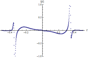
The current for a single ring is computed in the absence of wire . The current was computed for a fixed chemical potential, this explains the jump of the current at . In the presence of the Majorana energy in figure we obtain a shift in the persistent current with respect the single ring .For the Majorana energy the shift in the persistent current is reduced (the jump of the current originate from the fixed chemical potential as seen for the single ring). When the Majorana energy goes to zero the only contribution to the persistent current comes from the single ring . This dependence is due to the ground state energy which changes with the flux. In the presence of a Majorana Fermion we have in addition to the persistent current which comes from the perfect wire contributions like a contribution from the matrix which is a function of the Majorana energy determines and determines shift of the persistent current.
The persistent current is measured by the scanning of the SQUID [26] which measures the change in the magnetization. The magnetization is proportional to the persistent current. One subtracts from the persistent current contribution from the single ring and find the dependence on the Majorana energy. In the past only measurements of few rings was possible . In recent years some of the experimental groups have claimed to measure the persistent current in a single ring. Some of the complications are related to the fact that the measurements have been done in diffusive limit (with 10-20 rings) and not in the ballistic limit which we assumed in our calculation. The effect of the diffusive limit ca be study by coupling the rings to a noise bath.
8. Surface Physics-Photoemission
One of the ways to study the topology of the is to investigate the zero modes. The surface states zero modes (edge states ) for a have an odd number of chiral modes . The surface mode for the is given by one chiral mode, which is the Weyl Hamiltonian [30]. The conduction electrons have a fixed chirality on the surface of the . One observes topological surface excitations which are characterized by the integrated Fermi surface Berry curvature of . As a result, localization is prohibited [30]. The optical conductivity, the Raman spectrum, the polarization of the photoeletrons and the photoconductivity can reveal the topology of the surface states and spin texture. Recently the use of an innovative spectrometer with a high laser-based light source has shown that the spin polarization of the photoelectrons emitted from the surface of the Topological Insulator () can be manipulated through the laser light polarization [44]. One finds that the photoelectrons polarization is completely different from the initial states and is controlled by the photon polarization. The interpretation of these experiments are based on the assumption that the surface of the is flat. We will to compute the detection of photoelectrons and photoconductivity for an arbitrary a crystal-face boundary. We will introduce a model for photoemission for for an arbitrary surface.
8.1. Surface states for an arbitrary crystal-face boundary
Photoemmision, photoconductivity, optical conductivity and scanning tunneling microscopy are sensitive to the nature of the surface states. The topology of the surface states is affected by the physical boundary. For an arbitrary surface we need to solve the problem using a curved coordinate bases which rotates from point to point. For this type of problems the non-coordinate bases , introduced by Cartan [8, 9] is related to the Cartesian directions , . For example a point on a surface is given by the vector and by the coordinates on a surface with the normal to the surface . The two sets of coordinates are related throught the matrix , and . The normal to the surface is given by . This set of transformations allows to replace by the covariant derivative (which depends on the connection defined below) ; , and are the transformation and the inverse transformation matrix and are the connection one form matrix (see [8] page 285).
We will consider first the Weyl Hamiltonian for cylindrical coordinates (this problems has been considered in the literature [53, 54, 13]and here we will introduce a different method in order to deal with the arbitrary crystal face boundary.
The Weyl Hamiltonian in Cartesian coordinates is :.
We put the Hamiltonian on a cylinder and take the axes ; and ; . We propose to study this problem using the non-coordinate basis given by Cartan [8]: , and is the coordinate in the normal direction ; the derivatives are ; ; and the differentials (one form) are given by: ; ; . The coordinate basis is not fixed, therefore connection will be generated. The connection are determined from the Cartan’s structure equation for the Torsion : , . The connection is expanded in terms of the differential one form with the help of the matrix transformation : ; ; ; ;
From the transformation we obtain : and
From the torsion condition we find: , ( is the wedge product [8]) . We obtain the equation: ;.
the Weyl Hamiltonian in the cylindrical basis is given by:
The eigenvalue equation has real solutions for boundary conditions . We find: ; , ; ;;
8.2. The Hamiltonian for crystal face with a cylindrical boundary
In order to understand why the curved coordinates emerge, we will consider a three dimensional with the mass dependent gap is in the direction. Such a has a surface boundary perpendicular to the axes with crystal-face plane localized at . To simplify the discussion, we consider a situation where the crystal-face is cylindrical with the cylindrical axis in the direction and length . As a result, any point on the surface of the cylinder is given by the set of coordinates . The four-band model for the three dimensional , [6] of size . is given by where are the Pauli matrix for the orbitals and represents the spin:
;
The mass is a function of , , where is the step function. We have for , , therefore we obtain a zero mode on the surface, given by the two dimensional Weyl Hamiltonian on the surface . For a crystal-face which is cylindrical, any point on the cylinder makes an angle of with the axis.
We consider a situation where the surface perpendicular to axis (the direction of the mass gap is given by ) is is a surface of a cylinder. Any point on the surface can be viewed as rotated by an angle (the new ax makes an angle with the original axis for which the mass gap has been introduced ) The axes becomes the radial direction on a cylinder. The transformed Hamiltonian is expressed in terms of the covariant derivative . and are given by :
The Hamiltonian has zero mode solutions , where is given as a product of a scalar function and the spinor . The scalar function is localized at and vanishes for . Using the eigenvalues of and we find:
; ;
Using the eigenvectors and we introduce the rotated Pauli matrices , and for the orbital part Using the eigenstates we compute the projections ; and find the Hamiltonian for each point :
We observed that the rotation of the crystal-face for a cylinder is different from the surface state of a cylinder. In particular we mention the change sign Hamiltonian for a large angle, . We will compute the eigenvectors for eq. and determine the surface properties such as spin texture, and surface currents which affect the Photoemmision, the photoconductivity and the optical conductivity.
Conclusions To conclude the method of curved spaces in momentum space has been introduced. The method has been used to derive topological invariants from response theory. The theory has been applied to topological insulators topological superconductors and persistent currents. We have also studied the effect of the curved surfaces on the photoemission spectrum.
References
- [1] B.A.Volkov and O.A. Pankratov ”Two dimensional massless electrons in an inverted contact” JETP LETT. vol.42,179(1985)
- [2] F.D.M. Haldane ”Model For Quantum Hall Without Landau Levels ” Phys.Rev.Lett.61,2015(1988).
- [3] M.F.L.Golterman, K.Jansen and D.B. Kaplan ”Chern-Simons Currents and Chiral Fermions on the Lattice ” Phys.Lett.B301, (1993)219-223.
- [4] Michael Creutz and Ivan Horwath ”Surface States and Chiral Symmetry On The Lattice” Phys.Rev.D50,2297(1994)
- [5] C.L. Kane and E.J. Mele ”Quantum Spin Hall Effect In Graphene ” Phys.Rev. Lett. 95 226801 (2005)
- [6] C.L. Kane and E.J. Mele ” Topological Order And The Quantum Spin Hall Effect ”Phys.Rev.Lett. 95,146802(2005).
- [7] D.Schmeltzer,”Topological Spin Current Induced By Non-Commuting Coordinates: An application to the Spin-Hall Effect ”Phys.Rev.B 73,165301(2006).
- [8] M.Nakahara, ”Geometry,Topology and Physics” Taylor and Francis Group ,New York ,London (2003)
- [9] H.T. Nieh ”Gauss-Bonnet and Bianchi identities in Riemann-Cartan type gravitational theories” J.Math.Phys.21(6), June 1980
- [10] J.E.Moore and L.Balents ”Topological Invariants of Time-Reversal-Invariant Band Structures” Phys.Rev.B 75,121306(2007)
- [11] J. W. McIver, D. Hsieh, H. Steinberg ,PJarillo-Herrero and N.Gedik ,Nat.Nanotech ”Control over topological Insulator photocurrents with light polarization” 7,96 (2011).
- [12] Andrew M. Essin Joel E.Moore and David Vanderbilt ”Magnetoelectric Polarizability and Axion Electrodynamics In Cristalline Insulators” Phys.Rev.Lett.102,146805(2009)
- [13] M.M.Vazifeh and M.Franz ”Quantization and 2 periodicity of axion action in topological insulators”’Phys.Rev.B82,233103(2010)
- [14] D.A.Ivanov ”Non-Abelian of Half-Quantum Vortices in a p-Wave Superconductors” Phys.Rev.Lett.86,268(2001)
- [15] D.Schmeltzer and A.Saxena, ”Chiral P-wave Superconducting nanowire coupled to two metallic rings pierced by a flux ” Phys.Rev.B.86, 094519(2012).
- [16] Xiao-Liang Qi, Taylor Hughes and Shou-Cheng Zhang ”Topological Field Theory Of Time Reversal Invariant Insulators” Phys.Rev.B78,195424(2008)
- [17] Xiao-Liang Qi and Shou-Cheng Zhang ”Topological Insulators and Superconductors” Rev.of Modern Physics 831057 (2011).
- [18] Andreas P.Schnyder , Shinsei Ryu, Akira Furusaki, Andreas W.W. Ludwig ”Classification Of Topological Insulators and Superconductors In Three Spatial dimensions” Phys.Rev.B78,195125(2008)
- [19] M.Z.Hasan and J.E. Moore ”Three -dimensional topological Insulators” Anual Review of condensed matter Physics ,2:55,(2011)
- [20] J.G.Checkelsky,R.Yoshimi,A. Tsukazaki, K.S.Takahashi ”Trajectory of Anomalous Hall Effect toward the Quantized State in a Ferromagnetic Topological Insulator” arXiv:1406.7450v1
- [21] Chao-Xing Liu et al, ”Model Hamiltonian for Topological Insulators ” Physical Review B 82, 045122 (2010)
- [22] D.Schmeltzer , ”Quantum Mechanics For Genus g=2 Persistent Current in Coupled Rings”J. Phys:Condens Matter 20 335205(2008).
- [23] Steven Weinberg ”Theory Quantum Theory of Fields - volume II” (pages 445-450 ,eq.23.4.1) ,Cambridge University Press (1996)
- [24] D.Schmeltzer and A.Saxena ”Magnetoelectric effect induced by electron-electron interaction in three dimensional topological Insulators ” Physics Letters A 377 (2013) 1631-1636
- [25] D.Schmeltzer and A.Saxena ”The wave functions in the presence of constraints-persistent Current in Coupled Rings ” Phys.Rev.B 81 ,195310 (2010).
- [26] Hendryik Bluhm, Nicholas C. Koshnick, Julie A.Bert, Martin E.Hubert and Kathryin A.Moler ” Persistent currents in normal metal rings” Phys.Rev.Lett.102,136802 (2009)
- [27] D.Schmeltzer ”A-Geometrical approach to topological insulators with edge dislocations ” New Journal of Physics 14,063025 (2012)
- [28] D. Schmeltzer, ”Topological Insulators-transport in curved space” , arXiv:1012.5871 and Advances in Condensed Matter and Materials Research ,volume 10 Editors:Hans Geelvinck and Sjaak Reyst ,chapter 9, pages 379-403(2011).
- [29] D.Schmeltzer ”Propagation of Phonon in Topological Superconductors induced by strain fields instantons” International Journal of Modern Physics B vol.28,1450059 (2014)
- [30] D.Schmeltzer and Avadh Saxena ” Interference effects for time reversal invariant topological insulators : Surface Optical and Raman conductivity” Phys.Rev.B 88,035140 (2013)
- [31] Zohar Ringel ,Yaacov E.Kraus, and Ady Stern ”Strong side of weak topological insulators” Phys.Rev.B86,045102(2012)
- [32] E.I. Blount ”‘Formalism of Band Theory”’ Solid State Physics edited by F.Seitz and D. Turnubul , (Academic, New York ,1962),Vol.13, pages 305-375.
- [33] M.V.Berry ”Quantal Phase Factors Accompanying Adiabatic Changes” ,Proc.R.Soc.A392,45(1984).
- [34] D.Thouless,M.Kohmoto,M.Nightingale et M.den.Nijs, ”Quantized Hall Conductance In a Two-Dimensional Periodic Potential” Phys.Rev.Lett.49, 405 (1982).
- [35] B.Simon ”Holonomy the Quantum Adiabatic Theorem and Berry Phase ” Phys.Rev.Lett.51,2167 (1983).
- [36] J.Bellissard , Ordinary Quantum Hall Effect and Non-Commutativity Differential Geometry, in Localization in Disordered Systems, edited by Ziesche Weller ,Teubner -Verlag ,Leipzig ,(1987)
- [37] E.Prodan (2013) ”Quantum Transport :A Study Based on Operator Algebras ”Applied Mathematics Research eXpress, Vol.2013,No.2 pp.176-255. doi:10 .1093/amrx/abs017
- [38] V.Gourarie ”Single - particle Green’s functions and interacting topological insulators” Phys.Rev.83,085426 (2011)
- [39] Zhong Wang and Shou-Cheng Zhang ”Simplified Topological Invariants for Interacting Insulators” arXiv:1203.1028v3
- [40] Anndrew P.Schneider and Shinsei Ryu ”Topological phases and surface flat bands in superconductors whithout inversion symmetry” Phys.Rev.B. 84,060504(R)(2011)
- [41] Liang Fu ”Topological Crystalline Insulators” Phys.Rev.Lett.106,106802(2011)
- [42] Timothy H.Hsieh, Hsin Liu, Wenhui Duan, Arun Bansil and Liang Fu ” Topological crystalline insulators in the SnTe material classes ” arXiv: 1202.1003 v2
- [43] Michael Stone and Paul Goldbart ”Mathematics for Physics -A guided tour for graduate students ”, page 433 eq.12.63 , Cambridge University Press (2009)
- [44] Chris Jozwiak , Cheol-Hwan Park ,Keneth Gotlieb, Choongyu Hwang, Dung-Hai Lee , Steven G.Louie, Jonathan D. Denlinger , Costel R. Rotundu, Robert J. Birgeneau ,Zahid Hussainand Ale Lanzara, ”Photoelectron spin flipping and texture manipulation in topological insulator ” Nature Physics 293, vol 9 May (2013).
- [45] Fan Zhang,C.L. Kane, and E.J. Mele , ”Surface States of Topological Insulators ” Phys. Rev.B 86,081303(R)(2012)
- [46] Wu.C.B., A. Bernewig and Shou-Cheng Zhang ”‘The Helical Liquid and The Edge Of Quantum Spin Hall Systems”’ Phys.Rev.Lett. 96, 106401 (2006).
- [47] Chao-Xing Liu, X.L. Qi, H.Zhang,Xi Dai,Z. Fang and Shou-Cheng-Zhang ”Model Hamiltonian for topological insulators” Phys.Rev.B 82,045122(2010)
- [48] Chao-Xing Liu ,H.Zhang ,B.Yan, X.L. Qi, T.Frauenheim ,Xi Dai, Z. Fang and Shou-Cheng-Zhang ”Oscillatory crossover from two dimensional to three-dimensional topological insulators” Phys.Rev.B 81041307R (2010)
- [49] Shinobu Hikami ,”Anderson localization in a nonlinear -sigma model representation ” Phys.Rev.B 24,2671(1981)
- [50] A.A.Taskin,S.sasaki ,K.Segawa and Y. Ando ,”Quantum Oscillations in a Topological Insulator” Phys.Rev.Lett. 109,066803 (2012)
- [51] Hai-Zhou Lu, Junren Shi, and Shun-Qing Shen, ” Competition between localization and antilocalization in topological surface states ” Phys.Rev.Lett.107,076801(2011)
- [52] H.Peng et.al ”Aharonov-Bohhm interference in Topological Insulator Nanoribbons ” Nature Materials,9, 225 -229 (2010)
- [53] Yi Zhang and Ashvin Viswanath ”Anomalous Aharonov -Bohm
- [54] T.Hanaguri et al. ”Momentum-Resolved Ladau Level Spectroscopy of Dirac Surface States ”Phys.Rev.Lett.82,081305(2010)
- [55] R.Biswas and A.V. Balatsky ”Impurity-Induced On The Surface Of the Three -Dimensional Topological Insulator ” Phys.Rev.B 81,23405 (2010)
- [56] J.Chen, X.Y. He, K.H. Wu, Z.Q.Ji,L.Lu,J.R. Shi,J.H.Smet and Y.Q.Li”Tunable surface conductivity in revealed in diffusion electron transport” Phys.Rev.B. 83,241304(R)(2011)
- [57] I.Alicea,” New directions in the pursuit of Majorana fermions in solid state systems”, Rep. Prog. Phys. 75,076501 (2012).
- [58] B.Andrei Bernevig and Taylor L.Hughes ”Topological Insulators and Superconductors ” 2013 Princeton University Press,Princeton and Oxford.
- [59] D.Schmeltzer ”A microscopic model for detecting the surface states in Topological Insulators” arXiv:1310.6798(2013)
- [60] J. Zak, ”Berry Phase for energy Bands In Solids”, Phys. Rev. Lett. 62, 2747 (1989) .
- [61] Shinsey Riu, Joel Moore and Andreas W.W. Ludwig, ” Electromagnetic and gravitational responses and anomalies in topological insulators and superconductors ” Phys.Rev.B 85,045104 (2012)
- [62] Zhong Wang Xiao-Liang Qi and Shou-Cheng Zhang, ”Topological field theory and thermal responses of interacting topological superconductors ” Phys.Rev. B 84,014527(2011)