跳到论文正文
W Papers独立论文阅读器 arXiv:1012.5723 论文正文 计算阅读时间 · 0%
引用这篇论文根据当前论文元数据生成,正式投稿前建议核对。


License: arXiv.org perpetual non-exclusive license
arXiv:1012.5723v3 [cs.NI] 22 Jun 2011

Towards a Better Understanding of Large Scale Network Models

Guoqiang Mao    Senior Member, IEEE ††thanks: G. Mao is with the School of Electrical and Information Engineering, the University of Sydney and National ICT Australia. Email: guoqiang.mao@sydney.edu.au.    Brian D.O. Anderson    Life Fellow, IEEE ††thanks: B.D.O. Anderson is with the Research School of Information Sciences and Engineering, Australian National University and National ICT Australia. Email: brian.anderson@anu.edu.au.††thanks: This research is funded by ARC Discovery project: DP0877562.
Abstract

Connectivity and capacity are two fundamental properties of wireless multi-hop networks. The scalability of these properties has been a primary concern for which asymptotic analysis is a useful tool. Three related but logically distinct network models are often considered in asymptotic analyses, viz. the dense network model, the extended network model and the infinite network model, which consider respectively a network deployed in a fixed finite area with a sufficiently large node density, a network deployed in a sufficiently large area with a fixed node density, and a network deployed in ℜ2\Re^{2} with a sufficiently large node density. The infinite network model originated from continuum percolation theory and asymptotic results obtained from the infinite network model have often been applied to the dense and extended networks. In this paper, through two case studies related to network connectivity on the expected number of isolated nodes and on the vanishing of components of finite order k>1k>1 respectively, we demonstrate some subtle but important differences between the infinite network model and the dense and extended network models. Therefore extra scrutiny has to be used in order for the results obtained from the infinite network model to be applicable to the dense and extended network models. Asymptotic results are also obtained on the expected number of isolated nodes, the vanishingly small impact of the boundary effect on the number of isolated nodes and the vanishing of components of finite order k>1k>1 in the dense and extended network models using a generic random connection model.

Index Terms:
Dense network model, extended network model, infinite network model, continuum percolation, connectivity, random connection model

I Introduction

Wireless multi-hop networks in various forms, e.g. wireless ad hoc networks, sensor networks, mesh networks and vehicular networks, have been the subject of intense research in the recent decades (see [1] and references therein). Connectivity and capacity are two fundamental properties of these networks. The scalability of these properties as the number of nodes in the network becomes sufficiently large has been a primary concern. Asymptotic analysis, valid when the number of nodes in the network is large enough, has been useful for understanding the characteristics of these networks.

Three related but logically distinct network models have been widely used in the asymptotic analysis of large scale multi-hop networks. The first model, often referred to as the dense network model, considers that the network is deployed in a finite area with a sufficiently large node density. The second model, often referred to as the extended network model, considers that the node density is fixed and the network area is sufficiently large. The third model, referred to as the infinite network model, has its origin in continuum percolation theory [2]. It considers a network deployed in an infinite area, i.e. ℜ2\Re^{2} in 2D, and analyzes the properties of the network as the node density becomes sufficiently large. Due to the relatively longer history of research into continuum percolation theory and relatively abundant results in that area, and the close connections between the infinite network model and the dense and extended network models, results obtained in the infinite network model are often applied straightforwardly to the first and second models [3, 4, 5, 6, 7, 8].

In this paper, through two case studies on key events related to the network connectivity, i.e. the expected number of isolated nodes and the vanishing of components of fixed and finite order k>1k>1 (the order of a component refers to the number of nodes in the component), using a random connection model, we demonstrate some subtle but important differences between the infinite network model and the dense and extended network models due to the truncation effect, to be explained in the following paragraphs. Therefore results obtained from an infinite network model cannot be directly applied to the dense and extended networks. Instead some careful analysis of the impact of the truncation effect is required.

Here we give a detailed explanation of the above comments using a unit disk connection model as an example11 1 In the paper, we have omitted some trivial discussions on the difference between Poisson and uniform distributions and consider Poisson node distribution only.. Under the unit disk connection model, two nodes are directly connected if and only if (iff) their Euclidean distance is smaller than or equal to a given threshold r⁡(ρ)r\left(\rho\right), a parameter which is often taken as a function of a further parameter ρ\rho, to be defined shortly, under the dense and extended network models; the parameter r⁡(ρ)r\left(\rho\right) is termed the transmission range. The dense and extended network models that are often considered assume respectively a) nodes are Poissonly distributed in a unit area, say a square, with density ρ\rho and r⁡(ρ)=log⁡ρ+cπ​ρr\left(\rho\right)=\sqrt{\frac{\log\rho+c}{\pi\rho}} (the dense network model); b) nodes are Poissonly distributed on a square ρ×ρ\sqrt{\rho}\times\sqrt{\rho} with density 1 and r⁡(ρ)=log⁡ρ+cπr\left(\rho\right)=\sqrt{\frac{\log\rho+c}{\pi}} (the extended network model). The parameter cc may be either a constant; or it can depend on ρ\rho, in which case c=o⁡(log⁡ρ)c=o\left(\log\rho\right). The corresponding infinite network model considers nodes Poissonly distributed in ℜ2\Re^{2} with density ρ\rho and a pair of nodes are directly connected iff their Euclidean distance is smaller than or equal to rr, which does not depend on ρ\rho. The dense network model can be converted into the extended network model by scaling the Euclidean distances between all pairs of nodes by a factor of ρ\sqrt{\rho} while maintaining their connections, and conversely. Therefore the dense network model and the extended network model are equivalent in the analysis of connectivity. In the extended network model, as ρ→∞\rho\rightarrow\infty, the network area approaches ℜ2\Re^{2} and the average node degree approaches infinity following Θ⁡(log⁡ρ)\Theta\left(\log\rho\right), i.e. a node has more and more connections as ρ→∞\rho\rightarrow\infty. This resembles the situation that occurs in the infinite network model as ρ→∞\rho\rightarrow\infty. This close connection between the infinite network model and the dense and extended network models creates the illusion that as ρ→∞\rho\rightarrow\infty results obtained in the infinite network model can also be applied directly to the dense and extended models, e.g. those dealing with the vanishing of isolated nodes, the uniqueness of the component of infinite order, the vanishing of components of finite order k>1k>1 [3, 4, 5, 6, 7, 8].

Starting from the dense network model however, if we scale the Euclidean distances between all pairs of nodes by a factor 1/log⁡ρ+cπ​ρ1/\sqrt{\frac{\log\rho+c}{\pi\rho}}, there results a network on a square 1/log⁡ρ+cπ​ρ×1/log⁡ρ+cπ​ρ1/\sqrt{\frac{\log\rho+c}{\pi\rho}}\times 1/\sqrt{\frac{\log\rho+c}{\pi\rho}} with node density log⁡ρ+cπ\frac{\log\rho+c}{\pi}, where log⁡ρ+cπ→∞\frac{\log\rho+c}{\pi}\rightarrow\infty as ρ→∞\rho\rightarrow\infty, and a pair of nodes are directly connected iff their Euclidean distance is equal to or smaller than r=1r=1, independently of the node density. This latter network model is also equivalent to the dense and extended network models in connectivity. On the other hand, this latter network can also be obtained from an infinite network on ℜ2\Re^{2} with node density log⁡ρ+cπ\frac{\log\rho+c}{\pi} and r=1r=1 by removing all nodes and the associated connections outside a square of 1/log⁡ρ+cπ​ρ×1/log⁡ρ+cπ​ρ1/\sqrt{\frac{\log\rho+c}{\pi\rho}}\times 1/\sqrt{\frac{\log\rho+c}{\pi\rho}} in ℜ2\Re^{2}. We term the effect associated with the above removal procedure as the truncation effect. From the above discussion, it is clear that a prerequisite for the results obtained in the infinite network model to be applicable to the dense or extended network models is that the impact of the truncation effect on the property concerned must be vanishingly small as ρ→∞\rho\rightarrow\infty.

The main contributions of this paper are:

  • •

    Through two case studies, one on the expected number of isolated nodes and the other on the vanishing of components of fixed and finite order k>1k>1, using a random connection model, we show however that ensuring the impact of the truncation effect is vanishingly small either requires imposing a stronger requirement on the connection function or needs some non-trivial analysis to rule out the possibility of occurrence of some events associated with the truncation effect. Therefore results obtained assuming an infinite network model cannot be applied directly to the dense and extended network models.

  • •

    In particular, we show that in order for the impact of the truncation effect on the number of isolated nodes to be vanishingly small, a stronger requirement on the connection function (than the usual requirements of rotational invariance, integral boundedness and non-increasing monotonicity) needs to be imposed.

  • •

    We show that some non-trivial analysis is required to rule out the possibility of occurrence of some events associated with the truncation effect in order to establish the result on the vanishing of components of components of fixed and finite order k>1k>1 in the dense and extended network models. For example, an infinite component in ℜ2\Re^{2} may, after truncation, yield multiple components of extremely large order22 2 It is trivial to show that for any finite ρ\rho, almost surely there is no infinite component in a network whose nodes are Poissonly distributed with density log⁡ρ+cπ\frac{\log\rho+c}{\pi} on a square of 1/log⁡ρ+cπ​ρ×1/log⁡ρ+cπ​ρ1/\sqrt{\frac{\log\rho+c}{\pi\rho}}\times 1/\sqrt{\frac{\log\rho+c}{\pi\rho}}. Therefore we use the term components of extremely large order to refer to those components whose order may become asymptotically infinite as ρ→∞\rho\rightarrow\infty., finite components of fixed order k>1k>1 and isolated nodes in 1/log⁡ρ+cπ​ρ×1/log⁡ρ+cπ​ρ1/\sqrt{\frac{\log\rho+c}{\pi\rho}}\times 1/\sqrt{\frac{\log\rho+c}{\pi\rho}}, where these components are only connected via nodes and associated connections in the infinite component but outside 1/log⁡ρ+cπ​ρ×1/log⁡ρ+cπ​ρ1/\sqrt{\frac{\log\rho+c}{\pi\rho}}\times 1/\sqrt{\frac{\log\rho+c}{\pi\rho}}. Thus the dense and extended networks may still possibly have finite components of order k>1k>1 even though the infinite network can be shown to asymptotically almost surely have no such finite components as ρ→∞\rho\rightarrow\infty.

  • •

    Asymptotic results are established on the expected number of isolated nodes, the vanishingly small impact of the boundary effect on the number of isolated nodes and the vanishing of components of finite order k>1k>1 in the dense and extended network models using a generic random connection model. These results form key steps in extending asymptotic results on network connectivity from the unit disk model to the more generic random connection model.

To our knowledge, this is the first paper that has provided solid theoretical analysis to explain the difference between the infinite network model and the dense and extended network models and the cause of this difference, i.e. it is attributable to the truncation effect, which is different from the boundary effect that has been widely studied.

The rest of the paper is organized as follows. Section II reviews related work. Section III gives a formal definition of the network models, symbols and notations considered in the paper. Section IV comparatively studies the expected number of isolated nodes in a dense (or extended) network and in its counterpart infinite network model. Through the study, it shows that under certain conditions the impact of the truncation effect on the expected number of isolated nodes is non-negligible or may even be the dominant factor. Section V first gives an example to show that asymptotic vanishing of components of fixed and finite order k>1k>1 in an infinite network does not carry straightforwardly the conclusion that components of fixed and finite order k>1k>1 also vanish asymptotically in the dense and extended networks. Then to fill this theoretical gap and with a supplementary condition holding, a result is presented on the asymptotic vanishing of components of fixed and finite order k>1k>1 in the dense and extended network models under a random connection model. Finally Section VI summarizes conclusions and future work.

II Related Work

Extensive research has been done on connectivity problems using the well-known random geometric graph and the unit disk connection model, which is usually obtained by randomly and uniformly distributing nn vertices in a given area and connecting any two vertices iff their distance is smaller than or equal to a given threshold r⁡(n)r(n) [9, 10]. Significant outcomes have been obtained [3, 11, 12, 13, 14, 15, 10, 16].

Penrose [17, 18] and Gupta et al. [3] proved using different techniques that if the transmission range is set to r⁡(n)=log⁡n+c⁡(n)π​nr\left(n\right)=\sqrt{\frac{\log n+c\left(n\right)}{\pi n}}, a random network formed by uniformly placing nn nodes in a unit-area disk in ℜ2\Re^{2} is asymptotically almost surely connected as n→∞n\rightarrow\infty iff c⁡(n)→∞c\left(n\right)\rightarrow\infty. Specifically, Penrose’s result is based on the fact that in the above random network as ρ→∞\rho\rightarrow\infty the longest edge of the minimum spanning tree converges in probability to the minimum transmission range required for the above random network to have no isolated nodes (or equivalently the longest edge of the nearest neighbor graph of the above network) [17, 18, 10]. Gupta and Kumar’s result is based on a key finding in continuum percolation theory [2, Chapter 6]: Consider an infinite network with nodes distributed on ℜ2\Re^{2} following a Poisson distribution with density ρ\rho; and suppose that a pair of nodes separated by a Euclidean distance xx are directly connected with probability g⁡(x)g\left(x\right), independent of the event that another distinct pair of nodes are directly connected. Here, g:ℜ+→[0,1]g:\Re^{+}\rightarrow\left[0,1\right] satisfies the conditions of rotational invariance, non-increasing monotonicity and integral boundedness [2, pp. 151-152]. As ρ→∞\rho\rightarrow\infty asymptotically almost surely the above network on ℜ2\Re^{2} has only a unique infinite component and isolated nodes.

In [12], Philips et al. proved that the average node degree, i.e. the expected number of neighbors of an arbitrary node, must grow logarithmically with the area of the network to ensure that the network is connected, where nodes are placed randomly on a square according to a Poisson point process with a known density in ℜ2\Re^{2}. This result by Philips et al. actually provides a necessary condition on the average node degree required for connectivity. In [11], Xue et al. showed that in a network with a total of nn nodes randomly and uniformly distributed in a unit square in ℜ2\Re^{2}, if each node is connected to c​log⁡nc\log n nearest neighbors with c≤0.074c\leq 0.074 then the resulting random network is asymptotically almost surely disconnected as n→∞n\rightarrow\infty; and if each node is connected to c​log⁡nc\log n nearest neighbors with c≥5.1774c\geq 5.1774 then the network is asymptotically almost surely connected as n→∞n\rightarrow\infty. In [14], Balister et al. advanced the results in [11] and improved the lower and upper bounds to 0.3043​log⁡n0.3043\log n and 0.5139​log⁡n0.5139\log n respectively. In a more recent paper [16], Balister et al. achieved much improved results by showing that there exists a constant cc​r​i​tc_{crit} such that if each node is connected to ⌊c​log⁡n⌋\left\lfloor c\log n\right\rfloor nearest neighbors with c<cc​r​i​tc<c_{crit} then the network is asymptotically almost surely disconnected as n→∞n\rightarrow\infty, and if each node is connected to ⌊c​log⁡n⌋\left\lfloor c\log n\right\rfloor nearest neighbors with c>cc​r​i​tc>c_{crit} then the network is asymptotically almost surely connected as n→∞n\rightarrow\infty. In both [14] and [16], the authors considered nodes randomly distributed following a Poisson process of intensity one in a square of area nn in ℜ2\Re^{2}. In [13], Ravelomanana investigated the critical transmission range for connectivity in 3-dimensional wireless sensor networks and derived similar results to the 2-dimensional results in [3].

All the above work is based on the unit disk connection model. The unit disk connection model may simplify analysis but no real antenna has an antenna pattern similar to it. The log-normal shadowing connection model, which is more realistic than the unit disk connection model, has accordingly been considered for investigating network connectivity in [19, 20, 21, 22, 23, 24]. Under the log-normal shadowing connection model, two nodes are directly connected if the received power at one node from the other node, whose attenuation follows the log-normal model [25], is greater than a given threshold. In [19, 20, 21, 22, 23, 24], the authors investigated from different perspectives the necessary condition for a network with nodes uniformly or Poissonly distributed in a bounded area in ℜ2\Re^{2} and a pair of nodes are directly connected following the log-normal connection model to be connected. Most of the above work is based on the observation that a necessary condition for a connected network is that the network has no isolated nodes. Their analysis [19, 20, 21, 22, 23, 24] also relies on the assumption that under the log-normal connection model, the node isolation events are independent, an assumption yet to be validated analytically.

Other work in the area include [26, 6, 8, 5], which studies from the percolation perspective, the impact of mutual interference caused by simultaneous transmissions, the impact of physical layer cooperative transmissions, the impact of directional antennas and the impact of unreliable links on connectivity respectively.

In this paper we discuss the relation between three widely used network models in the above studies, i.e. the dense network model, the extended network model and the infinite network model which originated from continuum percolation theory. We examine mainly from the connectivity perspective the similarities and differences between these models and demonstrate that results obtained from continuum percolation theory assuming an infinite network model cannot be directly applied to the dense and extended network models. We also establish some results that form key steps in extending asymptotic results on network connectivity from the unit disk model to the more generic random connection model.

III Network Models

In this section we give a formal definition of network models considered in the paper. Let g:ℜ+→[0,1]g:\Re^{+}\rightarrow\left[0,1\right] be a function satisfying the conditions of non-increasing monotonicity and integral boundedness 33 3 Throughout this paper, we use the non-bold symbol, e.g. xx, to denote a scalar and the bold symbol, e.g. 𝒙\boldsymbol{x}, to denote a vector., 44 4 We refer readers to [27, 2, Chapter 6] for detailed discussions on the random connection model.:

g⁡(x)≤g⁡(y)\displaystyle g\left(x\right)\leq g\left(y\right) whenever​x≥y\displaystyle\textrm{whenever}\;\;x\geq y (1)
0<∫ℜ2g⁡(‖𝒙‖)​𝑑𝒙<∞\displaystyle 0<\int_{\Re^{2}}g\left(\left\|\boldsymbol{x}\right\|\right)d\boldsymbol{x}<\infty (2)

where ‖𝒙‖\left\|\boldsymbol{x}\right\| denotes the Euclidean norm of 𝒙\boldsymbol{x}. The function gg is the connection function that has been widely considered in the random connection model [27, 2, Chapter 6]. Further the requirement of rotational invariance on the connection function in the random connection model [27, 2, Chapter 6] has been met implicitly by letting gg be a function of a scalar, typically representing the Euclidean distance between two nodes being considered.

The following notations and definitions are used throughout the paper:

  • •

    f⁡(z)=oz​(h⁡(z))f\left(z\right)=o_{z}\left(h\left(z\right)\right) iff limz→∞f⁡(z)h⁡(z)=0\lim_{z\rightarrow\infty}\frac{f\left(z\right)}{h\left(z\right)}=0;

  • •

    f⁡(z)=ωz​(h⁡(z))f\left(z\right)=\omega_{z}\left(h\left(z\right)\right) iff h⁡(z)=oz​(f⁡(z))h\left(z\right)=o_{z}\left(f\left(z\right)\right);

  • •

    f⁡(z)=Θz​(h⁡(z))f\left(z\right)=\Theta_{z}\left(h\left(z\right)\right) iff there exist a sufficiently large z0z_{0} and two positive constants c1c_{1} and c2c_{2} such that for any z>z0z>z_{0}, c1​h​(z)≥f⁡(z)≥c2​h​(z)c_{1}h\left(z\right)\geq f\left(z\right)\geq c_{2}h\left(z\right);

  • •

    f(z)∼zh(z)f\left(z\right)\sim_{z}h\left(z\right) iff limz→∞f⁡(z)h⁡(z)=1\lim_{z\rightarrow\infty}\frac{f\left(z\right)}{h\left(z\right)}=1;

  • •

    An event ξ\xi is said to occur almost surely if its probability equals to one;

  • •

    An event ξz\xi_{z} depending on zz is said to occur asymptotically almost surely (a.a.s.) if its probability tends to one as z→∞z\rightarrow\infty.

The above definition applies whether the argument zz is continuous or discrete, e.g. assuming integer values.

Using the integral boundedness condition on gg and the non-increasing property of gg, it can be shown that

∫ℜ2g⁡(‖𝒙‖)​𝑑𝒙\displaystyle\int_{\Re^{2}}g\left(\left\|\boldsymbol{x}\right\|\right)d\boldsymbol{x} =\displaystyle= limz→∞∫0z2​π​x​g​(x)​𝑑x\displaystyle\lim_{z\rightarrow\infty}\int_{0}^{z}2\pi xg\left(x\right)dx

and

limz→∞∫z∞2​π​x​g​(x)​𝑑x=0\lim_{z\rightarrow\infty}\int_{z}^{\infty}2\pi xg\left(x\right)dx=0

The above equation, together with the following derivations

limz→∞∫z∞2​π​x​g​(x)​𝑑x\displaystyle\lim_{z\rightarrow\infty}\int_{z}^{\infty}2\pi xg\left(x\right)dx
≥\displaystyle\geq limz→∞∫z2​z2​π​x​g​(x)​𝑑x\displaystyle\lim_{z\rightarrow\infty}\int_{z}^{2z}2\pi xg\left(x\right)dx
≥\displaystyle\geq limz→∞∫z2​z2​π​x​g​(2​z)​𝑑x\displaystyle\lim_{z\rightarrow\infty}\int_{z}^{2z}2\pi xg\left(2z\right)dx
=\displaystyle= limz→∞3​π​z2​g​(2​z)\displaystyle\lim_{z\rightarrow\infty}3\pi z^{2}g\left(2z\right)

allow us to conclude that

g​(x)=ox​(1x2)g\left(x\right)=o_{x}\left(\frac{1}{x^{2}}\right) (3)

From time to time, we may require gg to satisfy the more restrictive requirement that

g​(x)=ox​(1x2​log2​x)g\left(x\right)=o_{x}\left(\frac{1}{x^{2}\log^{2}x}\right) (4)

and (1). When we do impose such additional constraint, we will specify it clearly. It is obvious that conditions (1) and (2) imply (3) while condition (4) implies (2) and (3).

In the following analysis, we will only use (1) and (4) (instead of (1) and (2)) when necessary. This helps to identify which part of the analysis relies on the more restrictive requirement on gg. In our analysis, we assume that gg has infinite support when necessary. Our results however apply to the situation when gg has bounded support, which forms a special case and only makes the analysis easier.

Further, define

rρ≜log⁡ρ+bC​ρr_{\rho}\triangleq\sqrt{\frac{\log\rho+b}{C\rho}} (5)

for some non-negative value ρ\rho, where

0<C=∫ℜ2g⁡(‖𝒙‖)​𝑑𝒙<∞0<C=\int_{\Re^{2}}g\left(\left\|\boldsymbol{x}\right\|\right)d\boldsymbol{x}<\infty (6)

and bb is a constant (+∞+\infty is allowed).

In the following, we give the formal definitions of four network models discussed in the paper. The motivation for defining a new model in Definition 3 appears later after all models are defined.

Definition 1

(dense network model) Let 𝒢⁡(𝒳ρ,grρ,A)\mathcal{G}\left(\mathcal{X}_{\rho},g_{r_{\rho}},A\right) be a network with nodes Poissonly distributed on a unit square A≜[−12,12]2A\triangleq\left[-\frac{1}{2},\frac{1}{2}\right]^{2} with density ρ\rho and a pair of nodes separated by a Euclidean distance xx are directly connected with probability grρ​(x)≜g​(xrρ)g_{r_{\rho}}\left(x\right)\triangleq g\left(\frac{x}{r_{\rho}}\right), independent of the event that another distinct pair of nodes are directly connected. 𝒳ρ\mathcal{X}_{\rho} denotes the vertex set in 𝒢⁡(𝒳ρ,grρ,A)\mathcal{G}\left(\mathcal{X}_{\rho},g_{r_{\rho}},A\right).

Definition 2

(extended network model) Let 𝒢⁡(𝒳1,glog⁡ρ+bC,Aρ)\mathcal{G}\left(\mathcal{X}_{1},g_{\sqrt{\frac{\log\rho+b}{C}}},A_{\sqrt{\rho}}\right) be a network with nodes Poissonly distributed on a square Aρ≜[−ρ2,ρ2]2A_{\sqrt{\rho}}\triangleq\left[-\frac{\sqrt{\rho}}{2},\frac{\sqrt{\rho}}{2}\right]^{2} with density 1 and a pair of nodes separated by a Euclidean distance xx are directly connected with probability glog⁡ρ+bC​(x)≜g⁡(xlog⁡ρ+bC)g_{\sqrt{\frac{\log\rho+b}{C}}}\left(x\right)\triangleq g\left(\frac{x}{\sqrt{\frac{\log\rho+b}{C}}}\right), independent of the event that another distinct pair of nodes are directly connected. 𝒳1\mathcal{X}_{1} denotes the vertex set in 𝒢⁡(𝒳1,glog⁡ρ+bC,Aρ)\mathcal{G}\left(\mathcal{X}_{1},g_{\sqrt{\frac{\log\rho+b}{C}}},A_{\sqrt{\rho}}\right).

Definition 3

Let 𝒢⁡(𝒳log⁡ρ+bC,g,A1rρ)\mathcal{G}\left(\mathcal{X}_{\frac{\log\rho+b}{C}},g,A_{\frac{1}{r_{\rho}}}\right) be a network with nodes Poissonly distributed on a square A1rρ≜[−12​rρ,12​rρ]2A_{\frac{1}{r_{\rho}}}\triangleq\left[-\frac{1}{2r_{\rho}},\frac{1}{2r_{\rho}}\right]^{2} with density log⁡ρ+bC\frac{\log\rho+b}{C} and a pair of nodes separated by a Euclidean distance xx are directly connected with probability g⁡(x)g\left(x\right), independent of the event that another distinct pair of nodes are directly connected. 𝒳log⁡ρ+bC\mathcal{X}_{\frac{\log\rho+b}{C}} denotes the vertex set in 𝒢⁡(𝒳log⁡ρ+bC,g,A1rρ)\mathcal{G}\left(\mathcal{X}_{\frac{\log\rho+b}{C}},g,A_{\frac{1}{r_{\rho}}}\right).

Definition 4

(infinite network model) Let 𝒢⁡(𝒳ρ,g,ℜ2)\mathcal{G}\left(\mathcal{X}_{\rho},g,\Re^{2}\right) be a network with nodes Poissonly distributed on ℜ2\Re^{2} with density ρ\rho and a pair of nodes separated by a Euclidean distance xx are directly connected with probability g⁡(x)g\left(x\right), independent of the event that another distinct pair of nodes are directly connected. 𝒳ρ\mathcal{X}_{\rho} denotes the vertex set in 𝒢⁡(𝒳ρ,g,ℜ2)\mathcal{G}\left(\mathcal{X}_{\rho},g,\Re^{2}\right).

With minor abuse of the terminology, we use AA (respectively AρA_{\sqrt{\rho}}, A1rρA_{\frac{1}{r_{\rho}}}) to denote both the square itself and the area of the square, and in the latter case, A=1A=1 (respectively Aρ=ρA_{\sqrt{\rho}}=\rho, A1rρ=1rρ2A_{\frac{1}{r_{\rho}}}=\frac{1}{r_{\rho}^{2}}).

The reason for choosing this particular form of rρr_{\rho} and the above network models is to avoid triviality in the analysis and to make the analysis compatible with existing results obtained under a unit disk connection model. Particularly when gg takes the form that g⁡(x)=1g(x)=1 for x≤1x\leq 1 and g⁡(x)=0g(x)=0 for x>1x>1, it can be shown that 𝒢⁡(𝒳ρ,grρ,A)\mathcal{G}\left(\mathcal{X}_{\rho},g_{r_{\rho}},A\right) reduces to the dense network model under a unit disk connection model discussed in [3, 10, 27] where C=πC=\pi and rρr_{\rho} corresponds to the critical transmission range for connectivity; 𝒢⁡(𝒳1,glog⁡ρ+bC,Aρ)\mathcal{G}\left(\mathcal{X}_{1},g_{\sqrt{\frac{\log\rho+b}{C}}},A_{\sqrt{\rho}}\right) reduces to the extended network model under a unit disk connection model considered in [28, 27, Chapter 3.3.2]. Thus the above model easily incorporates the unit disk connection model as a special case. A similar conclusion can also be drawn for the log-normal connection model.

Now we establish the relationship between the three network models in Definitions 1, 2, 3 on finite and then asymptotically infinite regions respectively using the scaling and coupling technique [2]. Given an instance of 𝒢⁡(𝒳ρ,grρ,A)\mathcal{G}\left(\mathcal{X}_{\rho},g_{r_{\rho}},A\right), if we scale the Euclidean distances between all pairs of nodes by a factor of ρ\sqrt{\rho} while maintaining their connections, there results a random network where nodes are Poissonly distributed on a square AρA_{\sqrt{\rho}} with density 11 and a pair of nodes separated by a Euclidean distance xx are directly connected with probability glog⁡ρ+bρ​(x)g_{\sqrt{\frac{\log\rho+b}{\rho}}}\left(x\right), i.e. an instance of 𝒢⁡(𝒳1,glog⁡ρ+bC,Aρ)\mathcal{G}\left(\mathcal{X}_{1},g_{\sqrt{\frac{\log\rho+b}{C}}},A_{\sqrt{\rho}}\right). All connectivity properties, e.g. connectivity, number of isolated nodes, number of components of a specified order, that hold in the instance of 𝒢⁡(𝒳ρ,grρ,A)\mathcal{G}\left(\mathcal{X}_{\rho},g_{r_{\rho}},A\right) are also valid for the associated instance in 𝒢⁡(𝒳1,glog⁡ρ+bC,Aρ)\mathcal{G}\left(\mathcal{X}_{1},g_{\sqrt{\frac{\log\rho+b}{C}}},A_{\sqrt{\rho}}\right) (To be more precise, the underlying graphs of these two network instances are isomorphic [29, 30]). Similarly if we shrink the Euclidean distances between all pairs of nodes in a network, which is an instance of 𝒢⁡(𝒳1,glog⁡ρ+bC,Aρ)\mathcal{G}\left(\mathcal{X}_{1},g_{\sqrt{\frac{\log\rho+b}{C}}},A_{\sqrt{\rho}}\right), by a factor of 1ρ\frac{1}{\sqrt{\rho}}, there results an instance of 𝒢⁡(𝒳ρ,grρ,A)\mathcal{G}\left(\mathcal{X}_{\rho},g_{r_{\rho}},A\right) and the two networks again have the same connectivity property. Therefore 𝒢⁡(𝒳ρ,grρ,A)\mathcal{G}\left(\mathcal{X}_{\rho},g_{r_{\rho}},A\right) and 𝒢⁡(𝒳1,glog⁡ρ+bC,Aρ)\mathcal{G}\left(\mathcal{X}_{1},g_{\sqrt{\frac{\log\rho+b}{C}}},A_{\sqrt{\rho}}\right) are equivalent in that any connectivity property that holds in one model will necessarily hold in the other. Similarly, it can also be shown that 𝒢⁡(𝒳ρ,grρ,A)\mathcal{G}\left(\mathcal{X}_{\rho},g_{r_{\rho}},A\right) and 𝒢⁡(𝒳log⁡ρ+bC,g,A1rρ)\mathcal{G}\left(\mathcal{X}_{\frac{\log\rho+b}{C}},g,A_{\frac{1}{r_{\rho}}}\right) are equivalent in their connectivity properties. Thus in this paper we only chose one model, i.e. 𝒢⁡(𝒳log⁡ρ+bC,g,A1rρ)\mathcal{G}\left(\mathcal{X}_{\frac{\log\rho+b}{C}},g,A_{\frac{1}{r_{\rho}}}\right), to discuss the connectivity properties of finite and asymptotically infinite networks. The reason for choosing this network model is that under the model, a pair of nodes are directly connected following gg, in the same way as nodes in the infinite network model 𝒢⁡(𝒳ρ,g,ℜ2)\mathcal{G}\left(\mathcal{X}_{\rho},g,\Re^{2}\right) are directly connected. This facilitates the discussion and comparison between the finite (asymptotically infinite) network model and the infinite network model, which is a key focus of the paper.

Further, we point out that the above discussion on the equivalence of network models 𝒢⁡(𝒳ρ,grρ,A)\mathcal{G}\left(\mathcal{X}_{\rho},g_{r_{\rho}},A\right), 𝒢⁡(𝒳1,glog⁡ρ+bC,Aρ)\mathcal{G}\left(\mathcal{X}_{1},g_{\sqrt{\frac{\log\rho+b}{C}}},A_{\sqrt{\rho}}\right) and 𝒢⁡(𝒳log⁡ρ+bC,g,A1rρ)\mathcal{G}\left(\mathcal{X}_{\frac{\log\rho+b}{C}},g,A_{\frac{1}{r_{\rho}}}\right) is only valid for the random connection model. For the other widely used model, i.e. the SINR model, under some special circumstances, e.g. the background noise is negligible [1] and the attenuation function is a power law function, the three network models are equivalent; otherwise under more general conditions, the three models are not equivalent (see e.g. [26, 31]). However the key observation revealed in our analysis, i.e. results obtained from an infinite network model do not necessarily apply to the dense and extended network models, also holds for the SINR model.

IV A Comparative Study of The Expected Number of Isolated Nodes

In this section we comparatively study the expected number of isolated nodes in 𝒢⁡(𝒳log⁡ρ+bC,g,A1rρ)\mathcal{G}\left(\mathcal{X}_{\frac{\log\rho+b}{C}},g,A_{\frac{1}{r_{\rho}}}\right) and the expected number of isolated nodes in its counterpart in an infinite network, i.e. a region with the same area as A1rρA_{\frac{1}{r_{\rho}}} in an infinite network on ℜ2\Re^{2} with the same node density log⁡ρ+bC\frac{\log\rho+b}{C} and connection function gg. The number of isolated nodes is a key parameter in the analysis of network connectivity. A necessary condition for a network to be connected is that the network has no isolated node. Such a necessary condition has been shown to be also a sufficient condition for a connected network as ρ→∞\rho\rightarrow\infty under a unit disk connection model [10] and this may also be possibly true for a random connection model.

IV-A Expected Number of Isolated Nodes in an Asymptotically Infinite Network

In this subsection we analyze the expected number of isolated nodes in 𝒢⁡(𝒳log⁡ρ+bC,g,A1rρ)\mathcal{G}\left(\mathcal{X}_{\frac{\log\rho+b}{C}},g,A_{\frac{1}{r_{\rho}}}\right). For an arbitrary node in 𝒢⁡(𝒳log⁡ρ+bC,g,A1rρ)\mathcal{G}\left(\mathcal{X}_{\frac{\log\rho+b}{C}},g,A_{\frac{1}{r_{\rho}}}\right) at location 𝒚\boldsymbol{y}, it can be shown that the probability that the node is isolated is given by [4]:

Pr(I𝒚=1)=e−∫A1rρlog⁡ρ+bCg(‖𝒙−𝒚‖)d𝒙\Pr\left(I_{\boldsymbol{y}}=1\right)=e^{-\int_{A_{\frac{1}{r_{\rho}}}}\frac{\log\rho+b}{C}g\left(\left\|\boldsymbol{x}-\boldsymbol{y}\right\|\right)d\boldsymbol{x}} (7)

where I𝒚I_{\boldsymbol{y}} is an indicator random variable: I𝒚=1I_{\boldsymbol{y}}=1 if the node at 𝒚\boldsymbol{y} is isolated and I𝒚=0I_{\boldsymbol{y}}=0 otherwise. Denote by WW the number of isolated nodes in an instance of 𝒢⁡(𝒳log⁡ρ+bC,g,A1rρ)\mathcal{G}\left(\mathcal{X}_{\frac{\log\rho+b}{C}},g,A_{\frac{1}{r_{\rho}}}\right). It then follows that the expected number of isolated nodes in 𝒢⁡(𝒳log⁡ρ+bC,g,A1rρ)\mathcal{G}\left(\mathcal{X}_{\frac{\log\rho+b}{C}},g,A_{\frac{1}{r_{\rho}}}\right) is given by

E(W)=∫A1rρlog⁡ρ+bCe−∫A1rρlog⁡ρ+bCg(‖𝒙−𝒚‖)d𝒙d𝒚E\left(W\right)=\int_{A_{\frac{1}{r_{\rho}}}}\frac{\log\rho+b}{C}e^{-\int_{A_{\frac{1}{r_{\rho}}}}\frac{\log\rho+b}{C}g\left(\left\|\boldsymbol{x}-\boldsymbol{y}\right\|\right)d\boldsymbol{x}}d\boldsymbol{y} (8)

On the basis of (8), the following theorem can be obtained.

Theorem 1

The expected number of isolated nodes in 𝒢⁡(𝒳log⁡ρ+bC,g,A1rρ)\mathcal{G}\left(\mathcal{X}_{\frac{\log\rho+b}{C}},g,A_{\frac{1}{r_{\rho}}}\right) is ∫A1rρlog⁡ρ+bCe−∫A1rρlog⁡ρ+bCg(‖𝐱−𝐲‖)d𝐱d𝐲\int_{A_{\frac{1}{r_{\rho}}}}\frac{\log\rho+b}{C}e^{-\int_{A_{\frac{1}{r_{\rho}}}}\frac{\log\rho+b}{C}g\left(\left\|\boldsymbol{x}-\boldsymbol{y}\right\|\right)d\boldsymbol{x}}d\boldsymbol{y}. For gg satisfying both (1) and (4), the expected number of isolated nodes in 𝒢⁡(𝒳log⁡ρ+bC,g,A1rρ)\mathcal{G}\left(\mathcal{X}_{\frac{\log\rho+b}{C}},g,A_{\frac{1}{r_{\rho}}}\right) converges asymptotically to e−be^{-b} as ρ→∞\rho\rightarrow\infty.

Proof:

See Appendix I ∎

IV-A1 Impact of Boundary Effect on the Number of Isolated Nodes

Before we proceed to the comparison of the expected number of isolated nodes in 𝒢⁡(𝒳log⁡ρ+bC,g,A1rρ)\mathcal{G}\left(\mathcal{X}_{\frac{\log\rho+b}{C}},g,A_{\frac{1}{r_{\rho}}}\right) and the expected number in its counterpart in an infinite network, we first examine the impact of boundary effect on the number of isolated nodes in 𝒢⁡(𝒳log⁡ρ+bC,g,A1rρ)\mathcal{G}\left(\mathcal{X}_{\frac{\log\rho+b}{C}},g,A_{\frac{1}{r_{\rho}}}\right). Boundary effect is a common concern in the analysis of network connectivity. The analysis of the impact of the boundary effect is done by comparing the number of isolated nodes in 𝒢⁡(𝒳log⁡ρ+bC,g,A1rρ)\mathcal{G}\left(\mathcal{X}_{\frac{\log\rho+b}{C}},g,A_{\frac{1}{r_{\rho}}}\right) and the number in a network with nodes Poissonly distributed on a torus A1rρT≜[−12​rρ,12​rρ]2A_{\frac{1}{r_{\rho}}}^{T}\triangleq\left[-\frac{1}{2r_{\rho}},\frac{1}{2r_{\rho}}\right]^{2} with node density log⁡ρ+bC\frac{\log\rho+b}{C} and where a pair of nodes separated by a toroidal distance xTx^{T} [10, p. 13] are directly connected with probability g⁡(xT)g\left(x^{T}\right), independent of the event that another distinct pair of nodes are directly connected. Denote the network on a torus by 𝒢T​(𝒳log⁡ρ+bC,g,A1rρT)\mathcal{G}^{T}\left(\mathcal{X}_{\frac{\log\rho+b}{C}},g,A_{\frac{1}{r_{\rho}}}^{T}\right). The following lemma can be established.

Lemma 1

The expected number of isolated nodes in 𝒢T​(𝒳log⁡ρ+bC,g,A1rρT)\mathcal{G}^{T}\left(\mathcal{X}_{\frac{\log\rho+b}{C}},g,A_{\frac{1}{r_{\rho}}}^{T}\right) is ρe−∫A1rρlog⁡ρ+bCg(‖𝐱‖)d𝐱\rho e^{-\int_{A_{\frac{1}{r_{\rho}}}}\frac{\log\rho+b}{C}g\left(\left\|\boldsymbol{x}\right\|\right)d\boldsymbol{x}}. For gg satisfying both (1) and (4), the expected number of isolated nodes in 𝒢T​(𝒳log⁡ρ+bC,g,A1rρ)\mathcal{G}^{T}\left(\mathcal{X}_{\frac{\log\rho+b}{C}},g,A_{\frac{1}{r_{\rho}}}\right) converges to e−be^{-b} as ρ→∞\rho\rightarrow\infty.

Proof:

See Appendix II ∎On the basis of Theorem 1 and Lemma 1, and using the coupling technique, the following lemma can be obtained.

Lemma 2

For gg satisfying both (1) and (4), the number of isolated nodes in 𝒢⁡(𝒳log⁡ρ+bC,g,A1rρ)\mathcal{G}\left(\mathcal{X}_{\frac{\log\rho+b}{C}},g,A_{\frac{1}{r_{\rho}}}\right) due to the boundary effect is a.a.s. 00 as ρ→∞\rho\rightarrow\infty.

Proof:

Comparing Theorem 1 and Lemma 1, it is noted that the expected numbers of isolated nodes on a torus and on a square respectively asymptotically converge to the same non-zero finite constant e−be^{-b} as ρ→∞\rho\rightarrow\infty. Now we use the coupling technique [2] to construct the connection between WW and WTW^{T}, the number of isolated nodes in the corresponding instance of 𝒢T​(𝒳log⁡ρ+bC,g,A1rρ)\mathcal{G}^{T}\left(\mathcal{X}_{\frac{\log\rho+b}{C}},g,A_{\frac{1}{r_{\rho}}}\right). Consider an instance of 𝒢T​(𝒳log⁡ρ+bC,g,A1rρT)\mathcal{G}^{T}\left(\mathcal{X}_{\frac{\log\rho+b}{C}},g,A_{\frac{1}{r_{\rho}}}^{T}\right). The number of isolated nodes in that network is WTW^{T}, which depends on ρ\rho. Remove each connection of the above network with probability 1−g⁡(x)g⁡(xT)1-\frac{g\left(x\right)}{g\left(x^{T}\right)}, independent of the event that another connection is removed, where xx is the Euclidean distance between the two endpoints of the connection and xTx^{T} is the corresponding toroidal distance. Due to xT≤xx^{T}\leq x (see (40) in Appendix II) and the non-increasing property of gg, 0≤1−g⁡(x)g⁡(xT)≤10\leq 1-\frac{g\left(x\right)}{g\left(x^{T}\right)}\leq 1. Further note that only connections between nodes near the boundary with xT<xx^{T}<x will be affected, i.e. when x=xTx=x^{T} the removal probability is zero. Denote the number of newly appearing isolated nodes by WEW^{E}. WEW^{E} has the meaning of being the number of isolated nodes due to the boundary effect. It is straightforward to show that WEW^{E} is a non-negative random integer, depending on ρ\rho. Further, such a connection removal process results a random network with nodes Poissonly distributed with density log⁡ρ+bC\frac{\log\rho+b}{C} where a pair of nodes separated by a Euclidean distance xx are directly connected with probability g⁡(x)g\left(x\right), i.e. a random network on a square with the boundary effect included. The following equation results as a consequence of the above discussion:

W=WE+WTW=W^{E}+W^{T}

Using Theorem 1, Lemma 1 and the above equation, it can be shown that

limρ→∞E⁡(WE)=limρ→∞E⁡(W−WT)=0\lim_{\rho\rightarrow\infty}E\left(W^{E}\right)=\lim_{\rho\rightarrow\infty}E\left(W-W^{T}\right)=0

Due to the non-negativity of WEW^{E}:

limρ→∞Pr⁡(WE=0)=1\lim_{\rho\rightarrow\infty}\Pr\left(W^{E}=0\right)=1

∎

Remark 1

Note that for gg not satisfying (4), E⁡(W)E\left(W\right) and E⁡(WT)E\left(W^{T}\right) are not necessarily convergent as ρ→∞\rho\rightarrow\infty. Particularly using the same procedure in Appendix I and II (see also (14) in Section IV-C below), it can be shown that when g​(x)=ωx​(1x2​log2​x)g\left(x\right)=\omega_{x}\left(\frac{1}{x^{2}\log^{2}x}\right), both limρ→∞E⁡(W)\lim_{\rho\rightarrow\infty}E\left(W\right) and limρ→∞E⁡(WT)\lim_{\rho\rightarrow\infty}E\left(W^{T}\right) are unbounded. When g​(x)=Θx​(1x2​log2​x)g\left(x\right)=\Theta_{x}\left(\frac{1}{x^{2}\log^{2}x}\right), limρ→∞E⁡(W)\lim_{\rho\rightarrow\infty}E\left(W\right) and limρ→∞E⁡(WT)\lim_{\rho\rightarrow\infty}E\left(W^{T}\right) start to depend on the asymptotic behavior of gg and is only convergent when limx→∞g⁡(x)​x2​log2​x=a\lim_{x\rightarrow\infty}g\left(x\right)x^{2}\log^{2}x=a, where 0<a<∞0<a<\infty is a positive constant. In that case, it can be shown that limρ→∞E⁡(W)\lim_{\rho\rightarrow\infty}E\left(W\right) and limρ→∞E⁡(WT)\lim_{\rho\rightarrow\infty}E\left(W^{T}\right) converge to e−b+4​πC​ae^{-b+\frac{4\pi}{C}a}. For limρ→∞E⁡(WT)\lim_{\rho\rightarrow\infty}E\left(W^{T}\right) the above result can be established by first choosing a small positive constant △​ε\triangle\varepsilon and then letting ρ\rho be sufficiently large such that D⁡(𝟎,12​rρ−1−△​ε)D\left(\boldsymbol{0},\frac{1}{2}r_{\rho}^{-1-\triangle\varepsilon}\right) contains A1rρA_{\frac{1}{r_{\rho}}}, where D⁡(𝐱,r)D\left(\boldsymbol{x},r\right) denotes a disk centered at 𝐱\boldsymbol{x} and with a radius rr. An upper and lower bound on E⁡(WT)E\left(W^{T}\right) can then be established by noting that

limρ→∞ρe−∫D⁡(𝟎,12​rρ−1−△​ε)log⁡ρ+bCg(‖𝒙‖)d𝒙\displaystyle\lim_{\rho\rightarrow\infty}\rho e^{-\int_{D\left(\boldsymbol{0},\frac{1}{2}r_{\rho}^{-1-\triangle\varepsilon}\right)}\frac{\log\rho+b}{C}g\left(\left\|\boldsymbol{x}\right\|\right)d\boldsymbol{x}}
≤\displaystyle\leq limρ→∞E(WT)=ρe−∫A1rρlog⁡ρ+bCg(‖𝒙‖)d𝒙\displaystyle\lim_{\rho\rightarrow\infty}E\left(W^{T}\right)=\rho e^{-\int_{A_{\frac{1}{r_{\rho}}}}\frac{\log\rho+b}{C}g\left(\left\|\boldsymbol{x}\right\|\right)d\boldsymbol{x}}
≤\displaystyle\leq limρ→∞ρe−∫D⁡(𝟎,12​rρ−1)log⁡ρ+bCg(‖𝒙‖)d𝒙\displaystyle\lim_{\rho\rightarrow\infty}\rho e^{-\int_{D\left(\boldsymbol{0},\frac{1}{2}r_{\rho}^{-1}\right)}\frac{\log\rho+b}{C}g\left(\left\|\boldsymbol{x}\right\|\right)d\boldsymbol{x}}

Following the exactly same procedure as that in (45) and (46) (in Appendix II) and finally letting △​ε→0\triangle\varepsilon\rightarrow 0, the result for limρ→∞E⁡(WT)\lim_{\rho\rightarrow\infty}E\left(W^{T}\right) can be obtained. The result for limρ→∞E⁡(W)\lim_{\rho\rightarrow\infty}E\left(W\right) can be obtained following a similar procedure as that in Appendix I.

IV-B The Number of Isolated Nodes in a Region A1rρA_{\frac{1}{r_{\rho}}} of an Infinite Network with Node Density log⁡ρ+bC\frac{\log\rho+b}{C}

In this subsection, we consider the number of isolated nodes in the counterpart of 𝒢⁡(𝒳log⁡ρ+bC,g,A1rρ)\mathcal{G}\left(\mathcal{X}_{\frac{\log\rho+b}{C}},g,A_{\frac{1}{r_{\rho}}}\right) in an infinite network. Specifically, for a meaningful comparison with the number of isolated nodes in 𝒢⁡(𝒳log⁡ρ+bC,g,A1rρ)\mathcal{G}\left(\mathcal{X}_{\frac{\log\rho+b}{C}},g,A_{\frac{1}{r_{\rho}}}\right), we consider the number of isolated nodes, denoted by W∞W^{\infty} (with superscript ∞ marking the parameter in an infinite network), in a square A1rρA_{\frac{1}{r_{\rho}}} of an infinite network on ℜ2\Re^{2} with Poissonly distributed node at density log⁡ρ+bC\frac{\log\rho+b}{C}. Denote the infinite network by 𝒢⁡(𝒳log⁡ρ+bC,g,ℜ2)\mathcal{G}\left(\mathcal{X}_{\frac{\log\rho+b}{C}},g,\Re^{2}\right). For gg satisfying (2), a randomly chosen node in 𝒢⁡(𝒳log⁡ρ+bC,g,ℜ2)\mathcal{G}\left(\mathcal{X}_{\frac{\log\rho+b}{C}},g,\Re^{2}\right), at location 𝒚∈A1rρ\boldsymbol{y}\in A_{\frac{1}{r_{\rho}}}, is isolated with probability

Pr(I𝒚∞=1)=e−∫ℜ2log⁡ρ+bCg(‖𝒙−𝒚‖)d𝒙=1ρe−b\Pr\left(I_{\boldsymbol{y}}^{\infty}=1\right)=e^{-\int_{\Re^{2}}\frac{\log\rho+b}{C}g\left(\left\|\boldsymbol{x}-\boldsymbol{y}\right\|\right)d\boldsymbol{x}}=\frac{1}{\rho}e^{-b} (9)

where (2) is used in the above equation. Therefore

E⁡(W∞)\displaystyle E\left(W^{\infty}\right) =\displaystyle= ∫A1rρlog⁡ρ+bC×1ρ​e−b​𝑑𝒚\displaystyle\int_{A_{\frac{1}{r_{\rho}}}}\frac{\log\rho+b}{C}\times\frac{1}{\rho}e^{-b}d\boldsymbol{y} (10)
=\displaystyle= log⁡ρ+bC×1ρ​e−b×(1rρ)2\displaystyle\frac{\log\rho+b}{C}\times\frac{1}{\rho}e^{-b}\times\left(\frac{1}{r_{\rho}}\right)^{2}
=\displaystyle= e−b\displaystyle e^{-b}

The last line follows by (5).

The above result is summarized in the following lemma:

Lemma 3

For gg satisfying (2), the expected number of isolated nodes in a region A1rρA_{\frac{1}{r_{\rho}}} of 𝒢⁡(𝒳log⁡ρ+bC,g,ℜ2)\mathcal{G}\left(\mathcal{X}_{\frac{\log\rho+b}{C}},g,\Re^{2}\right) is e−be^{-b}.

IV-C A Comparison of the Expected Number of Isolated Nodes in 𝒢⁡(𝒳log⁡ρ+bC,g,A1rρ)\mathcal{G}\left(\mathcal{X}_{\frac{\log\rho+b}{C}},g,A_{\frac{1}{r_{\rho}}}\right) and In Its Counterpart in An Infinite Network

Comparing Theorem 1 and Lemma 3, we note that:

  1. 1.

    The expected number of isolated nodes in 𝒢⁡(𝒳log⁡ρ+bC,g,A1rρ)\mathcal{G}\left(\mathcal{X}_{\frac{\log\rho+b}{C}},g,A_{\frac{1}{r_{\rho}}}\right) only converges asymptotically to e−be^{-b} as ρ→∞\rho\rightarrow\infty whereas the expected number of isolated nodes in an area of the same size in 𝒢⁡(𝒳log⁡ρ+bC,g,ℜ2)\mathcal{G}\left(\mathcal{X}_{\frac{\log\rho+b}{C}},g,\Re^{2}\right) is always e−be^{-b} no matter which value ρ\rho takes.

  2. 2.

    The expected number of isolated nodes in 𝒢⁡(𝒳log⁡ρ+bC,g,A1rρ)\mathcal{G}\left(\mathcal{X}_{\frac{\log\rho+b}{C}},g,A_{\frac{1}{r_{\rho}}}\right) converges asymptotically to e−be^{-b} for gg satisfying both (1) and (4) whereas the expected number of isolated nodes in an area of the same size in 𝒢⁡(𝒳log⁡ρ+bC,g,ℜ2)\mathcal{G}\left(\mathcal{X}_{\frac{\log\rho+b}{C}},g,\Re^{2}\right) is e−be^{-b} for gg satisfying (2) only.

In the following we examine the reason behind the differences.

Using (7), (8), (9) and (10), it can be shown that

E⁡(W)E⁡(W∞)\displaystyle\frac{E\left(W\right)}{E\left(W^{\infty}\right)}
=\displaystyle= eb∫A1rρlog⁡ρ+bCe−∫A1rρlog⁡ρ+bCg(‖𝒙−𝒚‖)d𝒙d𝒚\displaystyle e^{b}\int_{A_{\frac{1}{r_{\rho}}}}\frac{\log\rho+b}{C}e^{-\int_{A_{\frac{1}{r_{\rho}}}}\frac{\log\rho+b}{C}g\left(\left\|\boldsymbol{x}-\boldsymbol{y}\right\|\right)d\boldsymbol{x}}d\boldsymbol{y}
=\displaystyle= eb∫A1rρlog⁡ρ+bCexp(−∫ℜ2log⁡ρ+bCg(‖𝒙−𝒚‖)d𝒙\displaystyle e^{b}\int_{A_{\frac{1}{r_{\rho}}}}\frac{\log\rho+b}{C}\exp\left(-\int_{\Re^{2}}\frac{\log\rho+b}{C}g\left(\left\|\boldsymbol{x}-\boldsymbol{y}\right\|\right)d\boldsymbol{x}\right.
×\displaystyle\times OPEN∫ℜ2\A1rρlog⁡ρ+bC​g​(‖𝒙−𝒚‖)​𝑑𝒙)​𝑑𝒚\displaystyle\left.\int_{\Re^{2}\backslash A_{\frac{1}{r_{\rho}}}}\frac{\log\rho+b}{C}g\left(\left\|\boldsymbol{x}-\boldsymbol{y}\right\|\right)d\boldsymbol{x}\right)d\boldsymbol{y}
=\displaystyle= ∫A1rρlog⁡ρ+bC​ρ​e∫ℜ2\A1rρlog⁡ρ+bC​g​(‖𝒙−𝒚‖)​𝑑𝒙​𝑑𝒚\displaystyle\int_{A_{\frac{1}{r_{\rho}}}}\frac{\log\rho+b}{C\rho}e^{\int_{\Re^{2}\backslash A_{\frac{1}{r_{\rho}}}}\frac{\log\rho+b}{C}g\left(\left\|\boldsymbol{x}-\boldsymbol{y}\right\|\right)d\boldsymbol{x}}d\boldsymbol{y} (11)

It is trivial to show that the value in (11) is always greater than 11 for gg with infinite support. That is, for any gg with infinite support, the expected number of isolated nodes in 𝒢⁡(𝒳log⁡ρ+bC,g,A1rρ)\mathcal{G}\left(\mathcal{X}_{\frac{\log\rho+b}{C}},g,A_{\frac{1}{r_{\rho}}}\right) is strictly larger than the expected number of isolated nodes in an area A1rρA_{\frac{1}{r_{\rho}}} of 𝒢⁡(𝒳log⁡ρ+bC,g,ℜ2)\mathcal{G}\left(\mathcal{X}_{\frac{\log\rho+b}{C}},g,\Re^{2}\right). Further, it can be shown that the value in (11) accounts for the cumulative effect of nodes outside A1rρA_{\frac{1}{r_{\rho}}} in 𝒢⁡(𝒳log⁡ρ+bC,g,ℜ2)\mathcal{G}\left(\mathcal{X}_{\frac{\log\rho+b}{C}},g,\Re^{2}\right) and the associated connections between these nodes and nodes inside A1rρA_{\frac{1}{r_{\rho}}} on decreasing the expected number of isolated nodes in A1rρA_{\frac{1}{r_{\rho}}} respectively. Because 𝒢⁡(𝒳log⁡ρ+bC,g,A1rρ)\mathcal{G}\left(\mathcal{X}_{\frac{\log\rho+b}{C}},g,A_{\frac{1}{r_{\rho}}}\right) can be obtained from 𝒢⁡(𝒳log⁡ρ+bC,g,ℜ2)\mathcal{G}\left(\mathcal{X}_{\frac{\log\rho+b}{C}},g,\Re^{2}\right) by removing all these nodes and associated connections outside an area of A1rρA_{\frac{1}{r_{\rho}}} in 𝒢⁡(𝒳log⁡ρ+bC,g,ℜ2)\mathcal{G}\left(\mathcal{X}_{\frac{\log\rho+b}{C}},g,\Re^{2}\right), we term the this distinction the truncation effect. Theorem 1 and Lemma 3 shows that when gg satisfies both (1) and (4) (i.e. gg has to decrease fast enough), the impact of the truncation effect on isolated nodes becomes vanishingly small as ρ→∞\rho\rightarrow\infty.

Based on the above discussion, the following theorem can be established:

Theorem 2

For gg satisfying (2), the expected number of isolated nodes in an area of A1rρA_{\frac{1}{r_{\rho}}} in 𝒢⁡(𝒳log⁡ρ+bC,g,ℜ2)\mathcal{G}\left(\mathcal{X}_{\frac{\log\rho+b}{C}},g,\Re^{2}\right) is e−be^{-b}. Removing all nodes of 𝒢⁡(𝒳log⁡ρ+bC,g,ℜ2)\mathcal{G}\left(\mathcal{X}_{\frac{\log\rho+b}{C}},g,\Re^{2}\right) outside A1rρA_{\frac{1}{r_{\rho}}} and the associated connections, there results 𝒢⁡(𝒳log⁡ρ+bC,g,A1rρ)\mathcal{G}\left(\mathcal{X}_{\frac{\log\rho+b}{C}},g,A_{\frac{1}{r_{\rho}}}\right). The expected number of isolated nodes in 𝒢⁡(𝒳log⁡ρ+bC,g,A1rρ)\mathcal{G}\left(\mathcal{X}_{\frac{\log\rho+b}{C}},g,A_{\frac{1}{r_{\rho}}}\right) converges to e−be^{-b} if gg satisfies both (1) and (4). The more restrictive requirement on gg is a sufficient condition for the impact of the truncation effect associated with the above removal operations on the number of isolated nodes in 𝒢⁡(𝒳log⁡ρ+bC,g,A1rρ)\mathcal{G}\left(\mathcal{X}_{\frac{\log\rho+b}{C}},g,A_{\frac{1}{r_{\rho}}}\right) to be vanishingly small as ρ→∞\rho\rightarrow\infty.

In the following, we show that the more restrictive requirement on gg in (4) (compared with (1) and (2)) is also necessary for the impact of the truncation effect to become vanishingly small as ρ→∞\rho\rightarrow\infty. Specifically, consider the case when (4) is not satisfied. Let

f⁡(x)\displaystyle f\left(x\right) ≜\displaystyle\triangleq g⁡(x)​x2​log2​x\displaystyle g\left(x\right)x^{2}\log^{2}x (12)

Condition (4) not being satisfied means

limx→∞f⁡(x)≠0\lim_{x\rightarrow\infty}f\left(x\right)\neq 0 (13)

i.e. limx→∞f⁡(x)\lim_{x\rightarrow\infty}f\left(x\right) may equal to a positive constant, ∞\infty, or does not exist (e.g. f⁡(x)f\left(x\right) is a periodic function of xx).

It can be shown that (following the equation, detailed explanations are given and see also (42) in Appendix II)

limρ→∞E⁡(W)\displaystyle\lim_{\rho\rightarrow\infty}E\left(W\right) (14)
≥\displaystyle\geq limρ→∞E⁡(WT)\displaystyle\lim_{\rho\rightarrow\infty}E\left(W^{T}\right)
=\displaystyle= limρ→∞ρe−∫A1rρlog⁡ρ+bCg(‖𝒙‖)d𝒙\displaystyle\lim_{\rho\rightarrow\infty}\rho e^{-\int_{A_{\frac{1}{r_{\rho}}}}\frac{\log\rho+b}{C}g\left(\left\|\boldsymbol{x}\right\|\right)d\boldsymbol{x}}
≥\displaystyle\geq limρ→∞ρe−∫D⁡(𝟎,12​rρ−1)log⁡ρ+bCg(‖𝒙‖)d𝒙\displaystyle\lim_{\rho\rightarrow\infty}\rho e^{-\int_{D\left(\boldsymbol{0},\frac{1}{2}r_{\rho}^{-1}\right)}\frac{\log\rho+b}{C}g\left(\left\|\boldsymbol{x}\right\|\right)d\boldsymbol{x}}
=\displaystyle= e−b​limρ→∞e∫ℜ2\D⁡(𝟎,12​rρ−1)log⁡ρ+bC​g​(‖𝒙‖)​𝑑𝒙\displaystyle e^{-b}\lim_{\rho\rightarrow\infty}e^{\int_{\Re^{2}\backslash D\left(\boldsymbol{0},\frac{1}{2}r_{\rho}^{-1}\right)}\frac{\log\rho+b}{C}g\left(\left\|\boldsymbol{x}\right\|\right)d\boldsymbol{x}}
=\displaystyle= e−b+4​πC​limx→∞f⁡(x)\displaystyle e^{-b+\frac{4\pi}{C}\lim_{x\rightarrow\infty}f\left(x\right)}

where the last step results because of the following equation:

∫ℜ2\D⁡(𝟎,12​rρ−1)log⁡ρ+bC​g​(‖𝒙‖)​𝑑𝒙\displaystyle\int_{\Re^{2}\backslash D\left(\boldsymbol{0},\frac{1}{2}r_{\rho}^{-1}\right)}\frac{\log\rho+b}{C}g\left(\left\|\boldsymbol{x}\right\|\right)d\boldsymbol{x}
=\displaystyle= limρ→∞∫12​rρ−1∞log⁡ρ+bC​2​π​x​g​(x)​𝑑x\displaystyle\lim_{\rho\rightarrow\infty}\int_{\frac{1}{2}r_{\rho}^{-1}}^{\infty}\frac{\log\rho+b}{C}2\pi xg\left(x\right)dx
=\displaystyle= limρ→∞π2​rρ−4​g​(12​rρ−1)​log⁡ρ+b−1C​ρ2Cρ​(log⁡ρ+b)2\displaystyle\lim_{\rho\rightarrow\infty}\frac{\frac{\pi}{2}r_{\rho}^{-4}g\left(\frac{1}{2}r_{\rho}^{-1}\right)\frac{\log\rho+b-1}{C\rho^{2}}}{\frac{C}{\rho\left(\log\rho+b\right)^{2}}}
=\displaystyle= limρ→∞π2​C​(log⁡ρ+b)2​rρ−2​g​(12​rρ−1)\displaystyle\lim_{\rho\rightarrow\infty}\frac{\pi}{2C}\left(\log\rho+b\right)^{2}r_{\rho}^{-2}g\left(\frac{1}{2}r_{\rho}^{-1}\right)
=\displaystyle= limρ→∞π2​C​(log⁡ρ+b)2​rρ−2​f⁡(12​rρ−1)14​rρ−2​log2⁡(12​rρ−1)\displaystyle\lim_{\rho\rightarrow\infty}\frac{\pi}{2C}\left(\log\rho+b\right)^{2}r_{\rho}^{-2}\frac{f\left(\frac{1}{2}r_{\rho}^{-1}\right)}{\frac{1}{4}r_{\rho}^{-2}\log^{2}\left(\frac{1}{2}r_{\rho}^{-1}\right)}
=\displaystyle= limρ→∞2​π​(log⁡ρ+b)2​f​(12​rρ−1)C​(log⁡12−12​log⁡(log⁡ρ+b)+12​log​ρ+12​log​C)2\displaystyle\lim_{\rho\rightarrow\infty}\frac{2\pi\left(\log\rho+b\right)^{2}f\left(\frac{1}{2}r_{\rho}^{-1}\right)}{C\left(\log\frac{1}{2}-\frac{1}{2}\log\left(\log\rho+b\right)+\frac{1}{2}\log\rho+\frac{1}{2}\log C\right)^{2}}
=\displaystyle= 4​πC​limρ→∞f⁡(12​rρ−1)\displaystyle\frac{4\pi}{C}\lim_{\rho\rightarrow\infty}f\left(\frac{1}{2}r_{\rho}^{-1}\right)
=\displaystyle= 4​πC​limx→∞f⁡(x)\displaystyle\frac{4\pi}{C}\lim_{x\rightarrow\infty}f\left(x\right)

where in the second step, L’Hôpital’s rule with Clog⁡ρ+b\frac{C}{\log\rho+b} being the denominator and ∫12​rρ−1∞2​π​x​g​(x)​𝑑x\int_{\frac{1}{2}r_{\rho}^{-1}}^{\infty}2\pi xg\left(x\right)dx being the numerator is used; in the third step, (12) is used.

Remark 2

Equation (14) shows also that limρ→∞E⁡(WT)≥e−b+4​πC​limx→∞f⁡(x)\lim_{\rho\rightarrow\infty}E\left(W^{T}\right)\geq e^{-b+\frac{4\pi}{C}\lim_{x\rightarrow\infty}f\left(x\right)} where E⁡(WT)E\left(W^{T}\right) is the expected number of isolated nodes on a torus, which does not include the contribution of the boundary effect on the number of isolated nodes. Note also that the expected number of isolated nodes in an area of A1rρA_{\frac{1}{r_{\rho}}} in 𝒢⁡(𝒳log⁡ρ+bC,g,ℜ2)\mathcal{G}\left(\mathcal{X}_{\frac{\log\rho+b}{C}},g,\Re^{2}\right) is e−be^{-b}. Therefore the term e4​πC​limx→∞f⁡(x)e^{\frac{4\pi}{C}\lim_{x\rightarrow\infty}f\left(x\right)} is entirely attributable to the truncation effect.

Note that f⁡(x)f\left(x\right) is a non-negative function for x>1x>1. It is obvious from (14) that unless limx→∞f⁡(x)=0\lim_{x\rightarrow\infty}f\left(x\right)=0, i.e. (4) is satisfied, the expected number of isolated node in 𝒢⁡(𝒳log⁡ρ+bC,g,A1rρ)\mathcal{G}\left(\mathcal{X}_{\frac{\log\rho+b}{C}},g,A_{\frac{1}{r_{\rho}}}\right) will be larger than the expected number of isolated nodes in an area of A1rρA_{\frac{1}{r_{\rho}}} in 𝒢⁡(𝒳log⁡ρ+bC,g,ℜ2)\mathcal{G}\left(\mathcal{X}_{\frac{\log\rho+b}{C}},g,\Re^{2}\right). That is, the impact of the truncation effect on the number of isolated nodes in 𝒢⁡(𝒳log⁡ρ+bC,g,A1rρ)\mathcal{G}\left(\mathcal{X}_{\frac{\log\rho+b}{C}},g,A_{\frac{1}{r_{\rho}}}\right) will not be vanishingly small as ρ→∞\rho\rightarrow\infty. In particular, it can be shown that for g​(x)=Θx​(1x2​log2​x)g\left(x\right)=\Theta_{x}\left(\frac{1}{x^{2}\log^{2}x}\right), the impact of the truncation effect is non-negligible or even dominant in determining the number of isolated nodes in 𝒢⁡(𝒳log⁡ρ+bC,g,A1rρ)\mathcal{G}\left(\mathcal{X}_{\frac{\log\rho+b}{C}},g,A_{\frac{1}{r_{\rho}}}\right). Using (14), it can also be shown that for g​(x)=ωx​(1x2​log2​x)g\left(x\right)=\omega_{x}\left(\frac{1}{x^{2}\log^{2}x}\right), limρ→∞E⁡(W)\lim_{\rho\rightarrow\infty}E\left(W\right) is unbounded, i.e. connectivity cannot be achieved for g​(x)=ωx​(1x2​log2​x)g\left(x\right)=\omega_{x}\left(\frac{1}{x^{2}\log^{2}x}\right) even if (1) and (2) are satisfied.

The above discussion leads to the following conclusion:

Theorem 3

The more restrictive requirement on gg that it satisfies (4) is a necessary condition for the impact of the truncation effect on the number of isolated nodes in 𝒢⁡(𝒳log⁡ρ+bC,g,A1rρ)\mathcal{G}\left(\mathcal{X}_{\frac{\log\rho+b}{C}},g,A_{\frac{1}{r_{\rho}}}\right) to be vanishingly small as ρ→∞\rho\rightarrow\infty. Further for g​(x)=Θx​(1x2​log2​x)g\left(x\right)=\Theta_{x}\left(\frac{1}{x^{2}\log^{2}x}\right), the impact of the truncation effect is non-negligible or even dominant in determining the number of isolated nodes in 𝒢⁡(𝒳log⁡ρ+bC,g,A1rρ)\mathcal{G}\left(\mathcal{X}_{\frac{\log\rho+b}{C}},g,A_{\frac{1}{r_{\rho}}}\right); and for g​(x)=ωx​(1x2​log2​x)g\left(x\right)=\omega_{x}\left(\frac{1}{x^{2}\log^{2}x}\right), the truncation effect is the dominant factor in determining the number of isolated nodes in 𝒢⁡(𝒳log⁡ρ+bC,g,A1rρ)\mathcal{G}\left(\mathcal{X}_{\frac{\log\rho+b}{C}},g,A_{\frac{1}{r_{\rho}}}\right).

Noting that the number of isolated nodes in a network is a non-negative integer, the following result can be obtained as an easy consequence of Theorem 2 (see also [32]). Notice that in formulating this result, we drop the assumption that bb, originally introduced in (5), is a constant, and allow it instead to be ρ\rho-dependent.

Corollary 1

For gg satisfying both (1) and (4), a necessary condition for 𝒢⁡(𝒳log⁡ρ+bC,g,A1rρ)\mathcal{G}\left(\mathcal{X}_{\frac{\log\rho+b}{C}},g,A_{\frac{1}{r_{\rho}}}\right) to be a.a.s. (as ρ→∞\rho\rightarrow\infty) connected is b→∞b\rightarrow\infty.

Remark 3

As pointed out in [2, p. 151], the three requirements on gg in the random connection model, i.e. rotational invariance, non-increasing monotonicity and integral boundedness, are not equally important. Particularly, rotational invariance and non-increasing monotonicity are required only to simply the analysis such that “the notation and formulae will be somewhat simpler”. Similarly, we expect the results obtained in this section and in the next section requiring non-increasing monotonicity in (1) are also valid when the condition in (1) is removed. These however require more complicated handling of g⁡(x)g\left(x\right), particularly when xx is sufficiently large.

V Vanishing of Components of Finite Order

In this section we consider the events of the asymptotic vanishing of components of fixed and finite order k>1k>1 in the infinite network 𝒢⁡(𝒳log⁡ρ+bC,g,ℜ2)\mathcal{G}\left(\mathcal{X}_{\frac{\log\rho+b}{C}},g,\Re^{2}\right) and in 𝒢⁡(𝒳log⁡ρ+bC,g,A1rρ)\mathcal{G}\left(\mathcal{X}_{\frac{\log\rho+b}{C}},g,A_{\frac{1}{r_{\rho}}}\right) respectively as ρ→∞\rho\rightarrow\infty.

In [2, Theorem 6.4] it was shown that as ρ→∞\rho\rightarrow\infty (and log⁡ρ+bC→∞\frac{\log\rho+b}{C}\rightarrow\infty) the probability for a node to be isolated given that its component is finite converges to 11. In other words, as ρ→∞\rho\rightarrow\infty a.a.s. 𝒢⁡(𝒳log⁡ρ+bC,g,ℜ2)\mathcal{G}\left(\mathcal{X}_{\frac{\log\rho+b}{C}},g,\Re^{2}\right) has only isolated nodes and components of infinite order, and components of fixed and finite order k>1k>1 asymptotically vanish. In the following we show that due to the truncation effect, the above result obtained in 𝒢⁡(𝒳log⁡ρ+bC,g,ℜ2)\mathcal{G}\left(\mathcal{X}_{\frac{\log\rho+b}{C}},g,\Re^{2}\right) does not carry over to the conclusion that as ρ→∞\rho\rightarrow\infty a.a.s. 𝒢⁡(𝒳log⁡ρ+bC,g,A1rρ)\mathcal{G}\left(\mathcal{X}_{\frac{\log\rho+b}{C}},g,A_{\frac{1}{r_{\rho}}}\right) has only isolated nodes and infinite components too, without further analysis on the impact of the truncation effect. Specifically, an infinite component in 𝒢⁡(𝒳log⁡ρ+bC,g,ℜ2)\mathcal{G}\left(\mathcal{X}_{\frac{\log\rho+b}{C}},g,\Re^{2}\right) may possibly consist of components of extremely large order, components of fixed and finite order k>1k>1 and isolated nodes involving nodes and connections entirely contained inside A1rρA_{\frac{1}{r_{\rho}}}, where these components are only connected to each other via nodes and connections outside A1rρA_{\frac{1}{r_{\rho}}}. Note that for any finite ρ\rho, almost surely there is no infinite component in 𝒢⁡(𝒳log⁡ρ+bC,g,A1rρ)\mathcal{G}\left(\mathcal{X}_{\frac{\log\rho+b}{C}},g,A_{\frac{1}{r_{\rho}}}\right). Therefore we use the term component of extremely large order to refer to a component whose order may become asymptotically infinite as ρ→∞\rho\rightarrow\infty. As the nodes and associated connections outside A1rρA_{\frac{1}{r_{\rho}}} are removed, the infinite component in ℜ2\Re^{2} may possibly leave components of extremely large order, components of finite order k>1k>1 and isolated nodes in A1rρA_{\frac{1}{r_{\rho}}}. As such, vanishing of components of finite order k>1k>1 in 𝒢⁡(𝒳log⁡ρ+bC,g,ℜ2)\mathcal{G}\left(\mathcal{X}_{\frac{\log\rho+b}{C}},g,\Re^{2}\right) as ρ→∞\rho\rightarrow\infty does not necessarily carry the conclusion that components of finite order k>1k>1 in 𝒢⁡(𝒳log⁡ρ+bC,g,A1rρ)\mathcal{G}\left(\mathcal{X}_{\frac{\log\rho+b}{C}},g,A_{\frac{1}{r_{\rho}}}\right) also vanish as ρ→∞\rho\rightarrow\infty, even when A1rρA_{\frac{1}{r_{\rho}}} approaches ℜ2\Re^{2} as ρ→∞\rho\rightarrow\infty. An example is illustrated in Fig. 1.

Refer to caption
Figure 1: An illustration that an infinite component in ℜ2\Re^{2} may leave components of extremely large order, components of finite order k>1k>1 and isolated nodes in a finite (or asymptotically infinite) region in ℜ2\Re^{2} when nodes and connections outside the finite (asymptotically infinite) region is removed. The figure uses the unit disk connection model as a special case for easy illustration. Each ball has a radius of half of the transmission range and is centered at a node. Two adjacent balls overlap iff the associated nodes are directly connected. The figure shows an infinite component with nodes organized in a tree structure. The square area represents the finite (asymptotically infinite) region. Even as the square grows to include more and more nodes of the infinite component, it is still possible for the square to have components of finite order k>1k>1 when nodes and connections outside the square are removed.

We further point out that many other topologies, particularly under a random connection model where even a pair of nodes separated by a large distance may have a non-zero probability to be directly connected, can be drawn for an infinite component in ℜ2\Re^{2}, where after removing all nodes and associated connections of the infinite component outside A1rρA_{\frac{1}{r_{\rho}}}, the infinite component leaves components of finite order k>1k>1 inside A1rρA_{\frac{1}{r_{\rho}}}, even when A1rρA_{\frac{1}{r_{\rho}}} grows as ρ→∞\rho\rightarrow\infty. We emphasize that we are not hinting that the topology of the infinite component shown in Fig. 1 is likely to occur in 𝒢⁡(𝒳log⁡ρ+bC,g,ℜ2)\mathcal{G}\left(\mathcal{X}_{\frac{\log\rho+b}{C}},g,\Re^{2}\right) as ρ→∞\rho\rightarrow\infty, but neither can such a possibility be precluded using [2, Theorem 6.4]. Therefore a conclusion cannot be drawn straightforwardly from [2, Theorem 6.4] that a.a.s. components of finite order k>1k>1 in 𝒢⁡(𝒳log⁡ρ+bC,g,A1rρ)\mathcal{G}\left(\mathcal{X}_{\frac{\log\rho+b}{C}},g,A_{\frac{1}{r_{\rho}}}\right) vanish as ρ→∞\rho\rightarrow\infty. Instead some non-trivial analysis is required to establish such a conclusion in 𝒢⁡(𝒳log⁡ρ+bC,g,A1rρ)\mathcal{G}\left(\mathcal{X}_{\frac{\log\rho+b}{C}},g,A_{\frac{1}{r_{\rho}}}\right).

We present such a result for the vanishing of components of finite order k>1k>1 in 𝒢⁡(𝒳log⁡ρ+bC,g,A1rρ)\mathcal{G}\left(\mathcal{X}_{\frac{\log\rho+b}{C}},g,A_{\frac{1}{r_{\rho}}}\right) as ρ→∞\rho\rightarrow\infty to fill this theoretical gap:

Theorem 4

For gg satisfying (1) and (4), a.a.s. there is no component of finite order k>1k>1 in 𝒢⁡(𝒳log⁡ρ+bC,g,A1rρ)\mathcal{G}\left(\mathcal{X}_{\frac{\log\rho+b}{C}},g,A_{\frac{1}{r_{\rho}}}\right).

Proof:

See Appendix III.∎

Remark 4

Theorem 4 gives a sufficient condition on gg required for the number of components of fixed and finite order k>1k>1 in 𝒢⁡(𝒳log⁡ρ+bC,g,A1rρ)\mathcal{G}\left(\mathcal{X}_{\frac{\log\rho+b}{C}},g,A_{\frac{1}{r_{\rho}}}\right) to be vanishingly small as ρ→∞\rho\rightarrow\infty. It is also interesting to obtain a necessary condition on gg required for the number of components of fixed and finite order k>1k>1 in 𝒢⁡(𝒳log⁡ρ+bC,g,A1rρ)\mathcal{G}\left(\mathcal{X}_{\frac{\log\rho+b}{C}},g,A_{\frac{1}{r_{\rho}}}\right) to be vanishingly small. The technique used in the proof of Theorem 4 however cannot answer the above question on a necessary condition on gg. More specifically, denote by ξk\xi_{k} the (random) number of components of order kk in an instance of 𝒢⁡(𝒳λ,g,A1rρ)\mathcal{G}\left(\mathcal{X}_{\lambda},g,A_{\frac{1}{r_{\rho}}}\right) and let MM be an arbitrarily large positive integer MM. The proof of Theorem 4 is based on an analysis of E⁡(∑k=2Mξk)E\left(\sum_{k=2}^{M}\xi_{k}\right). By showing that limρ→∞E⁡(∑k=2Mξk)=0\lim_{\rho\rightarrow\infty}E\left(\sum_{k=2}^{M}\xi_{k}\right)=0, it follows that limρ→∞Pr⁡(∑k=2Mξk=0)=1\lim_{\rho\rightarrow\infty}\Pr\left(\sum_{k=2}^{M}\xi_{k}=0\right)=1. However limρ→∞E⁡(∑k=2Mξk)=0\lim_{\rho\rightarrow\infty}E\left(\sum_{k=2}^{M}\xi_{k}\right)=0 is only a sufficient condition for limρ→∞Pr⁡(∑k=2Mξk=0)=1\lim_{\rho\rightarrow\infty}\Pr\left(\sum_{k=2}^{M}\xi_{k}=0\right)=1, not a necessary condition. It would be interesting to develop a technique to obtain a tight necessary condition on gg required for the number of components of fixed and finite order k>1k>1 in 𝒢⁡(𝒳log⁡ρ+bC,g,A1rρ)\mathcal{G}\left(\mathcal{X}_{\frac{\log\rho+b}{C}},g,A_{\frac{1}{r_{\rho}}}\right) to be vanishingly small.

VI Conclusion

In this paper, we discussed the connectivity of several network models including the widely used dense network model 𝒢⁡(𝒳ρ,grρ,A)\mathcal{G}\left(\mathcal{X}_{\rho},g_{r_{\rho}},A\right), extended network model 𝒢⁡(𝒳1,glog⁡ρ+bC,Aρ)\mathcal{G}\left(\mathcal{X}_{1},g_{\sqrt{\frac{\log\rho+b}{C}}},A_{\sqrt{\rho}}\right) and infinite network model 𝒢⁡(𝒳ρ,g,ℜ2)\mathcal{G}\left(\mathcal{X}_{\rho},g,\Re^{2}\right). Using the scaling and coupling technique, it is shown that the dense network model and the extended network model are equivalent in their connectivity properties and they are also equivalent to the network model 𝒢⁡(𝒳log⁡ρ+bC,g,A1rρ)\mathcal{G}\left(\mathcal{X}_{\frac{\log\rho+b}{C}},g,A_{\frac{1}{r_{\rho}}}\right), which can be obtained from the infinite network model 𝒢⁡(𝒳log⁡ρ+bC,g,ℜ2)\mathcal{G}\left(\mathcal{X}_{\frac{\log\rho+b}{C}},g,\Re^{2}\right) by removing all nodes and associated connections outside the area A1rρA_{\frac{1}{r_{\rho}}} of 𝒢⁡(𝒳ρ,g,ℜ2)\mathcal{G}\left(\mathcal{X}_{\rho},g,\Re^{2}\right). Define the effect associated with the above removal operation as the truncation effect. A prerequisite for any (asymptotic) conclusion obtained in the infinite network model to be applicable to the dense and extended network models is that the impact of the truncation effect must be vanishingly small on the parameter concerned as ρ→∞\rho\rightarrow\infty - a conclusion that often needs non-trivial analysis to establish. We then conducted two case studies using a random connection model, on the expected number of isolated nodes and on the vanishing of components of fixed and finite order k>1k>1 respectively, with a focus on examining the impact of the truncation effect and showed that the connection function gg has to decrease sufficiently fast in order for the truncation effect to have a vanishingly small impact.

In the first case study, we showed that for gg satisfying both (1) and (4), the impact of the truncation effect on the number of isolated nodes in 𝒢⁡(𝒳log⁡ρ+bC,g,A1rρ)\mathcal{G}\left(\mathcal{X}_{\frac{\log\rho+b}{C}},g,A_{\frac{1}{r_{\rho}}}\right) is vanishingly small as ρ→∞\rho\rightarrow\infty. However for gg satisfying (1) and (2) only, the impact of the truncation effect on the number of isolated nodes in 𝒢⁡(𝒳log⁡ρ+bC,g,A1rρ)\mathcal{G}\left(\mathcal{X}_{\frac{\log\rho+b}{C}},g,A_{\frac{1}{r_{\rho}}}\right) is non-negligible and may even be the dominant factor in determining the number of isolated nodes.

In the second case study, we first showed using an example that due to the truncation effect, asymptotic vanishing of components of fixed and finite order k>1k>1 in an infinite network does not carry over straightforwardly to the conclusion that components of fixed and finite order k>1k>1 also vanish asymptotically in the dense and extended networks. Then to fill this theoretical gap, a result is presented on the asymptotic vanishing of components of finite order k>1k>1 in the dense and extended network models under a random connection model.

Some interesting results useful for the analysis of connectivity under a random connection model in the dense and extended networks were also established. These include the expected number of isolated nodes, which resulted in a necessary condition for a dense (or extended) network to be connected, the vanishingly small impact of the boundary effect on the number of isolated nodes, and the asymptotic vanishing of components of finite order k>1k>1.

Many results in the paper were given in the form of sufficient conditions on the connection function gg required for the impact of the truncation effect to be vanishingly small. It will be interesting and important to examine necessary conditions on gg required for the impact of the truncation effect to be vanishingly small.

Appendix I Proof of Theorem 1

In this Appendix, we give a proof of Theorem 1.

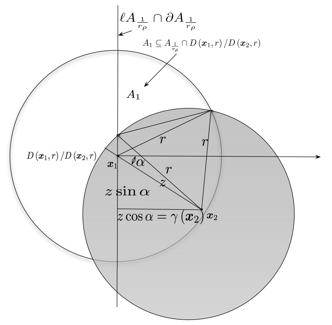
We analyze E⁡(W)E\left(W\right) as ρ→∞\rho\rightarrow\infty. Denote by D⁡(𝒚,rρ−ε)D\left(\boldsymbol{y},r_{\rho}^{-\varepsilon}\right) a disk centered at 𝒚\boldsymbol{y} and with a radius rρ−εr_{\rho}^{-\varepsilon}, where ε\varepsilon is a small positive constant and ε<14\varepsilon<\frac{1}{4}. Denote by B⁡(A1rρ)⊂A1rρB\left(A_{\frac{1}{r_{\rho}}}\right)\subset A_{\frac{1}{r_{\rho}}} an area within rρ−εr_{\rho}^{-\varepsilon} of the border of A1rρA_{\frac{1}{r_{\rho}}}; denote by ℓ​A1rρ⊂A1rρ\ell A_{\frac{1}{r_{\rho}}}\subset A_{\frac{1}{r_{\rho}}} a rectangular area of size rρ−ε×(rρ−1−2​rρ−ε)r_{\rho}^{-\varepsilon}\times\left(r_{\rho}^{-1}-2r_{\rho}^{-\varepsilon}\right) within rρ−εr_{\rho}^{-\varepsilon} of one side of A1rρA_{\frac{1}{r_{\rho}}}, away from the corners of A1rρA_{\frac{1}{r_{\rho}}} by rρ−εr_{\rho}^{-\varepsilon}, and there are four such areas; let ∠​A1rρ⊂A1rρ\angle A_{\frac{1}{r_{\rho}}}\subset A_{\frac{1}{r_{\rho}}} denote a square of size rρ−ε×rρ−εr_{\rho}^{-\varepsilon}\times r_{\rho}^{-\varepsilon} at the four corners of A1rρA_{\frac{1}{r_{\rho}}}. Fig. 2 illustrates these areas.

Refer to caption
Figure 2: An Illustration of the boundary areas of A1rρA_{\frac{1}{r_{\rho}}}. The areas ∠​A1rρ\angle A_{\frac{1}{r_{\rho}}}, ℓ​A1rρ\ell A_{\frac{1}{r_{\rho}}} are self-explanatory and B⁡(A1rρ)B\left(A_{\frac{1}{r_{\rho}}}\right) is the shaded area in the figure.

It follows from (8) that

limρ→∞E⁡(W)\displaystyle\lim_{\rho\rightarrow\infty}E\left(W\right) (15)
=\displaystyle= limρ→∞∫A1rρlog⁡ρ+bCe−∫A1rρlog⁡ρ+bCg(‖𝒙−𝒚‖)d𝒙d𝒚\displaystyle\lim_{\rho\rightarrow\infty}\int_{A_{\frac{1}{r_{\rho}}}}\frac{\log\rho+b}{C}e^{-\int_{A_{\frac{1}{r_{\rho}}}}\frac{\log\rho+b}{C}g\left(\left\|\boldsymbol{x}-\boldsymbol{y}\right\|\right)d\boldsymbol{x}}d\boldsymbol{y}
=\displaystyle= limρ→∞ρrρ2∫A1rρ\B⁡(A1rρ)e−ρrρ2∫A1rρg(‖𝒙−𝒚‖)d𝒙d𝒚\displaystyle\lim_{\rho\rightarrow\infty}\rho r_{\rho}^{2}\int_{A_{\frac{1}{r_{\rho}}}\backslash B\left(A_{\frac{1}{r_{\rho}}}\right)}e^{-\rho r_{\rho}^{2}\int_{A_{\frac{1}{r_{\rho}}}}g\left(\left\|\boldsymbol{x}-\boldsymbol{y}\right\|\right)d\boldsymbol{x}}d\boldsymbol{y}
+\displaystyle+ limρ→∞4ρrρ2∫ℓ​A1rρe−ρrρ2∫A1rρg(‖𝒙−𝒚‖)d𝒙d𝒚\displaystyle\lim_{\rho\rightarrow\infty}4\rho r_{\rho}^{2}\int_{\ell A_{\frac{1}{r_{\rho}}}}e^{-\rho r_{\rho}^{2}\int_{A_{\frac{1}{r_{\rho}}}}g\left(\left\|\boldsymbol{x}-\boldsymbol{y}\right\|\right)d\boldsymbol{x}}d\boldsymbol{y}
+\displaystyle+ limρ→∞4ρrρ2∫∠​A1rρe−ρrρ2∫A1rρg(‖𝒙−𝒚‖)d𝒙d𝒚\displaystyle\lim_{\rho\rightarrow\infty}4\rho r_{\rho}^{2}\int_{\angle A_{\frac{1}{r_{\rho}}}}e^{-\rho r_{\rho}^{2}\int_{A_{\frac{1}{r_{\rho}}}}g\left(\left\|\boldsymbol{x}-\boldsymbol{y}\right\|\right)d\boldsymbol{x}}d\boldsymbol{y}

The three summands in (15) represent respectively the expected number of isolated nodes in the central area A1rρ\B⁡(A1rρ)A_{\frac{1}{r_{\rho}}}\backslash B\left(A_{\frac{1}{r_{\rho}}}\right), in the boundary area along the four sides of A1rρA_{\frac{1}{r_{\rho}}} and in the four corners of A1rρA_{\frac{1}{r_{\rho}}}. In the following analysis, we will show that for gg satisfying both (1) and (4), the first term approaches e−be^{-b} as ρ→∞\rho\rightarrow\infty, and the second and the third terms approach 00 as ρ→∞\rho\rightarrow\infty.

Consider the first summand in (15). Using the definition of rρr_{\rho} in (5), first it can be shown that for any 𝒚\boldsymbol{y} and therefore 𝒚∈A1rρ\B⁡(A1rρ)\boldsymbol{y}\in A_{\frac{1}{r_{\rho}}}\backslash B\left(A_{\frac{1}{r_{\rho}}}\right) (see Fig. 2 for the region A1rρ\B⁡(A1rρ)A_{\frac{1}{r_{\rho}}}\backslash B\left(A_{\frac{1}{r_{\rho}}}\right)):

limρ→∞ρe−ρrρ2∫D⁡(𝒚,rρ−ε)g(‖𝒙−𝒚‖)d𝒙\displaystyle\lim_{\rho\rightarrow\infty}\rho e^{-\rho r_{\rho}^{2}\int_{D\left(\boldsymbol{y},r_{\rho}^{-\varepsilon}\right)}g\left(\left\|\boldsymbol{x}-\boldsymbol{y}\right\|\right)d\boldsymbol{x}} (16)
=\displaystyle= limρ→∞ρ​e−ρ​rρ2​(∫ℜ2g⁡(‖𝒙−𝒚‖)​𝑑𝒙−∫ℜ2\D⁡(𝒚,rρ−ε)g⁡(‖𝒙−𝒚‖)​𝑑𝒙)\displaystyle\lim_{\rho\rightarrow\infty}\rho e^{-\rho r_{\rho}^{2}\left(\int_{\Re^{2}}g\left(\left\|\boldsymbol{x}-\boldsymbol{y}\right\|\right)d\boldsymbol{x}-\int_{\Re^{2}\backslash D\left(\boldsymbol{y},r_{\rho}^{-\varepsilon}\right)}g\left(\left\|\boldsymbol{x}-\boldsymbol{y}\right\|\right)d\boldsymbol{x}\right)}
=\displaystyle= limρ→∞ρ​e−ρ​rρ2​(C−∫ℜ2\D⁡(𝒚,rρ−ε)g⁡(‖𝒙−𝒚‖)​𝑑𝒙)\displaystyle\lim_{\rho\rightarrow\infty}\rho e^{-\rho r_{\rho}^{2}\left(C-\int_{\Re^{2}\backslash D\left(\boldsymbol{y},r_{\rho}^{-\varepsilon}\right)}g\left(\left\|\boldsymbol{x}-\boldsymbol{y}\right\|\right)d\boldsymbol{x}\right)}
=\displaystyle= limρ→∞e−b​eρ​rρ2​∫ℜ2\D⁡(𝒚,rρ−ε)g⁡(‖𝒙−𝒚‖)​𝑑𝒙\displaystyle\lim_{\rho\rightarrow\infty}e^{-b}e^{\rho r_{\rho}^{2}\int_{\Re^{2}\backslash D\left(\boldsymbol{y},r_{\rho}^{-\varepsilon}\right)}g\left(\left\|\boldsymbol{x}-\boldsymbol{y}\right\|\right)d\boldsymbol{x}}
=\displaystyle= e−b​limρ→∞elog⁡ρ+bC​∫rρ−ε∞2​π​r​g​(r)​𝑑r\displaystyle e^{-b}\lim_{\rho\rightarrow\infty}e^{\frac{\log\rho+b}{C}\int_{r_{\rho}^{-\varepsilon}}^{\infty}2\pi rg\left(r\right)dr}

It can be shown further using (5) that (following the equation, detailed explanations are given):

limρ→∞log⁡ρ+bC​∫rρ−ε∞2​π​r​g​(r)​𝑑r\displaystyle\lim_{\rho\rightarrow\infty}\frac{\log\rho+b}{C}\int_{r_{\rho}^{-\varepsilon}}^{\infty}2\pi rg\left(r\right)dr
=\displaystyle= limρ→∞∫rρ−ε∞2​π​r​g​(r)​𝑑rClog⁡ρ+b\displaystyle\lim_{\rho\rightarrow\infty}\frac{\int_{r_{\rho}^{-\varepsilon}}^{\infty}2\pi rg\left(r\right)dr}{\frac{C}{\log\rho+b}}
=\displaystyle= limρ→∞−2​π​rρ−ε​g​(rρ−ε)​(−ε2​rρ−ε−2​1−(log⁡ρ+b)C​ρ2)−Cρ​(log⁡ρ+b)2\displaystyle\lim_{\rho\rightarrow\infty}\frac{-2\pi r_{\rho}^{-\varepsilon}g\left(r_{\rho}^{-\varepsilon}\right)\left(-\frac{\varepsilon}{2}r_{\rho}^{-\varepsilon-2}\frac{1-\left(\log\rho+b\right)}{C\rho^{2}}\right)}{-\frac{C}{\rho\left(\log\rho+b\right)^{2}}}
=\displaystyle= limρ→∞π​ε​(log⁡ρ+b)2​rρ−2​ε−2​g​(rρ−ε)​log⁡ρ+b−1C​ρ\displaystyle\lim_{\rho\rightarrow\infty}\pi\varepsilon\left(\log\rho+b\right)^{2}r_{\rho}^{-2\varepsilon-2}g\left(r_{\rho}^{-\varepsilon}\right)\frac{\log\rho+b-1}{C\rho}
=\displaystyle= limρ→∞π​ε​(log⁡ρ+b)2​rρ−2​ε​g​(rρ−ε)\displaystyle\lim_{\rho\rightarrow\infty}\pi\varepsilon\left(\log\rho+b\right)^{2}r_{\rho}^{-2\varepsilon}g\left(r_{\rho}^{-\varepsilon}\right) (17)
=\displaystyle= limρ→∞π​ε​(log⁡ρ+b)2​rρ−2​ε​oρ​(1rρ−2​ε​log2⁡(rρ−2​ε))\displaystyle\lim_{\rho\rightarrow\infty}\pi\varepsilon\left(\log\rho+b\right)^{2}r_{\rho}^{-2\varepsilon}o_{\rho}\left(\frac{1}{r_{\rho}^{-2\varepsilon}\log^{2}\left(r_{\rho}^{-2\varepsilon}\right)}\right) (18)
=\displaystyle= limρ→∞(π​ε​(log⁡ρ+b)2CLOSE\displaystyle\lim_{\rho\rightarrow\infty}\left(\pi\varepsilon\left(\log\rho+b\right)^{2}\right.
OPENoρ​(12​ε2​(log⁡(log⁡ρ+b)−log⁡C−log⁡ρ)2))\displaystyle\left.o_{\rho}\left(\frac{1}{2\varepsilon^{2}\left(\log\left(\log\rho+b\right)-\log C-\log\rho\right)^{2}}\right)\right)
=\displaystyle= 0\displaystyle 0 (19)

where L’Hôpital’s rule is used in the second step of the above equation, and g​(x)=ox​(1x2​log2​x)g\left(x\right)=o_{x}\left(\frac{1}{x^{2}\log^{2}x}\right) is used from (17) to (18). As a result of (16) and (19)

limρ→∞ρe−ρrρ2∫D⁡(𝒚,rρ−ε)g(‖𝒙−𝒚‖)d𝒙=e−b\lim_{\rho\rightarrow\infty}\rho e^{-\rho r_{\rho}^{2}\int_{D\left(\boldsymbol{y},r_{\rho}^{-\varepsilon}\right)}g\left(\left\|\boldsymbol{x}-\boldsymbol{y}\right\|\right)d\boldsymbol{x}}=e^{-b} (20)

It follows that (see Fig. 2 for an illustration of the region A1rρ\B⁡(A1rρ)A_{\frac{1}{r_{\rho}}}\backslash B\left(A_{\frac{1}{r_{\rho}}}\right), which is unshaded in the figure.)

limρ→∞ρrρ2∫A1rρ\B⁡(A1rρ)e−ρrρ2∫A1rρg(‖𝒙−𝒚‖)d𝒙d𝒚\displaystyle\lim_{\rho\rightarrow\infty}\rho r_{\rho}^{2}\int_{A_{\frac{1}{r_{\rho}}}\backslash B\left(A_{\frac{1}{r_{\rho}}}\right)}e^{-\rho r_{\rho}^{2}\int_{A_{\frac{1}{r_{\rho}}}}g\left(\left\|\boldsymbol{x}-\boldsymbol{y}\right\|\right)d\boldsymbol{x}}d\boldsymbol{y}
≤\displaystyle\leq limρ→∞ρrρ2∫A1rρ\B⁡(A1rρ)e−ρrρ2∫D⁡(𝒚,rρ−ε)g(‖𝒙−𝒚‖)d𝒙d𝒚\displaystyle\lim_{\rho\rightarrow\infty}\rho r_{\rho}^{2}\int_{A_{\frac{1}{r_{\rho}}}\backslash B\left(A_{\frac{1}{r_{\rho}}}\right)}e^{-\rho r_{\rho}^{2}\int_{D\left(\boldsymbol{y},r_{\rho}^{-\varepsilon}\right)}g\left(\left\|\boldsymbol{x}-\boldsymbol{y}\right\|\right)d\boldsymbol{x}}d\boldsymbol{y}
=\displaystyle= limρ→∞(ρe−ρrρ2∫D⁡(𝟎,rρ−ε)g(‖𝒙‖)d𝒙)(rρ2∫A1rρ\B⁡(A1rρ)d𝒚)\displaystyle\lim_{\rho\rightarrow\infty}\left(\rho e^{-\rho r_{\rho}^{2}\int_{D\left(\boldsymbol{0},r_{\rho}^{-\varepsilon}\right)}g\left(\left\|\boldsymbol{x}\right\|\right)d\boldsymbol{x}}\right)\left(r_{\rho}^{2}\int_{A_{\frac{1}{r_{\rho}}}\backslash B\left(A_{\frac{1}{r_{\rho}}}\right)}d\boldsymbol{y}\right)
=\displaystyle= e−b\displaystyle e^{-b}

and

limρ→∞ρrρ2∫A1rρ\B⁡(A1rρ)e−ρrρ2∫A1rρg(‖𝒙−𝒚‖)d𝒙d𝒚\displaystyle\lim_{\rho\rightarrow\infty}\rho r_{\rho}^{2}\int_{A_{\frac{1}{r_{\rho}}}\backslash B\left(A_{\frac{1}{r_{\rho}}}\right)}e^{-\rho r_{\rho}^{2}\int_{A_{\frac{1}{r_{\rho}}}}g\left(\left\|\boldsymbol{x}-\boldsymbol{y}\right\|\right)d\boldsymbol{x}}d\boldsymbol{y}
≥\displaystyle\geq limρ→∞ρrρ2∫A1rρ\B⁡(A1rρ)e−ρrρ2∫ℜ2g(‖𝒙−𝒚‖)d𝒙d𝒚\displaystyle\lim_{\rho\rightarrow\infty}\rho r_{\rho}^{2}\int_{A_{\frac{1}{r_{\rho}}}\backslash B\left(A_{\frac{1}{r_{\rho}}}\right)}e^{-\rho r_{\rho}^{2}\int_{\Re^{2}}g\left(\left\|\boldsymbol{x}-\boldsymbol{y}\right\|\right)d\boldsymbol{x}}d\boldsymbol{y}
=\displaystyle= e−b\displaystyle e^{-b}

Therefore

limρ→∞ρrρ2∫A1rρ/B⁡(A1rρ)e−ρrρ2∫A1rρg(‖𝒙−𝒚‖)d𝒙d𝒚=e−b\lim_{\rho\rightarrow\infty}\rho r_{\rho}^{2}\int_{A_{\frac{1}{r_{\rho}}}/B\left(A_{\frac{1}{r_{\rho}}}\right)}e^{-\rho r_{\rho}^{2}\int_{A_{\frac{1}{r_{\rho}}}}g\left(\left\|\boldsymbol{x}-\boldsymbol{y}\right\|\right)d\boldsymbol{x}}d\boldsymbol{y}=e^{-b} (21)

For the second term in (15), an illustration of the boundary area for 𝒚∈ℓ​A1rρ\boldsymbol{y}\in\ell A_{\frac{1}{r_{\rho}}} is shown in Fig. 3.

Refer to caption
(a)
Refer to caption
(b)
Figure 3: An illustration of the boundary area for 𝒚∈ℓ​A1rρ\boldsymbol{y}\in\ell A_{\frac{1}{r_{\rho}}}. The figure is drawn for 𝒚\boldsymbol{y} located near the left border of A1rρA_{\frac{1}{r_{\rho}}}. The situations for 𝒚\boldsymbol{y} near the top, bottom and right borders of A1rρA_{\frac{1}{r_{\rho}}} can be drawn analogously. D⁡(𝒚,rρ−ε)D\left(\boldsymbol{y},r_{\rho}^{-\varepsilon}\right) is a disk centered at 𝒚\boldsymbol{y} and has a radius rρ−εr_{\rho}^{-\varepsilon}. lyl_{y} is the distance between 𝒚\boldsymbol{y} and the border of A1rρA_{\frac{1}{r_{\rho}}}. DyD_{y} is a half disk centered at 𝒚\boldsymbol{y}, with a radius rρ−εr_{\rho}^{-\varepsilon} and on the right side of 𝒚\boldsymbol{y}. CyC_{y} is a half disk centered at 𝒚\boldsymbol{y}, with a radius lyl_{y} and on the left side of 𝒚\boldsymbol{y}. Ry⊂A1rρ∩D⁡(𝒚,rρ−ε)R_{y}\subset A_{\frac{1}{r_{\rho}}}\cap D\left(\boldsymbol{y},r_{\rho}^{-\varepsilon}\right) is a rectangle of ly×2​rρ−2​ε−ly2l_{y}\times 2\sqrt{r_{\rho}^{-2\varepsilon}-l_{y}^{2}} on the left side of 𝒚\boldsymbol{y}. Ly=(A1rρ∩D⁡(𝒚,rρ−ε))\DyL_{y}=\left(A_{\frac{1}{r_{\rho}}}\cap D\left(\boldsymbol{y},r_{\rho}^{-\varepsilon}\right)\right)\backslash D_{y} is the shaded area in sub-figure b.

Define Ly≜(A1rρ∩D⁡(𝒚,rρ−ε))\DyL_{y}\triangleq\left(A_{\frac{1}{r_{\rho}}}\cap D\left(\boldsymbol{y},r_{\rho}^{-\varepsilon}\right)\right)\backslash D_{y} (i.e. the shaded area in Fig. 3b). The symbols DyD_{y}, CyC_{y}, lyl_{y} and RyR_{y} are defined in Fig. 3. It can be shown that

4limρ→∞ρrρ2∫ℓ​A1rρe−ρrρ2∫A1rρg(‖𝒙−𝒚‖)d𝒙d𝒚\displaystyle 4\lim_{\rho\rightarrow\infty}\rho r_{\rho}^{2}\int_{\ell A_{\frac{1}{r_{\rho}}}}e^{-\rho r_{\rho}^{2}\int_{A_{\frac{1}{r_{\rho}}}}g\left(\left\|\boldsymbol{x}-\boldsymbol{y}\right\|\right)d\boldsymbol{x}}d\boldsymbol{y}
≤\displaystyle\leq 4limρ→∞rρ2∫ℓ​A1rρρe−ρrρ2∫A1rρ∩D⁡(𝒚,rρ−ε)g(‖𝒙−𝒚‖)d𝒙d𝒚\displaystyle 4\lim_{\rho\rightarrow\infty}r_{\rho}^{2}\int_{\ell A_{\frac{1}{r_{\rho}}}}\rho e^{-\rho r_{\rho}^{2}\int_{A_{\frac{1}{r_{\rho}}}\cap D\left(\boldsymbol{y},r_{\rho}^{-\varepsilon}\right)}g\left(\left\|\boldsymbol{x}-\boldsymbol{y}\right\|\right)d\boldsymbol{x}}d\boldsymbol{y}
=\displaystyle= 4​limρ→∞rρ2​∫ℓ​A1rρρ​e−ρ​rρ2​(∫Dyg⁡(‖𝒙−𝒚‖)​𝑑𝒙+∫Lyg⁡(‖𝒙−𝒚‖)​𝑑𝒙)​𝑑𝒚\displaystyle 4\lim_{\rho\rightarrow\infty}r_{\rho}^{2}\int_{\ell A_{\frac{1}{r_{\rho}}}}\rho e^{-\rho r_{\rho}^{2}\left(\int_{D_{y}}g\left(\left\|\boldsymbol{x}-\boldsymbol{y}\right\|\right)d\boldsymbol{x}+\int_{L_{y}}g\left(\left\|\boldsymbol{x}-\boldsymbol{y}\right\|\right)d\boldsymbol{x}\right)}d\boldsymbol{y}
=\displaystyle= 4limρ→∞((ρ12e−12ρrρ2∫D⁡(𝟎,rρ−ε)g(‖𝒙‖)d𝒙)\displaystyle 4\lim_{\rho\rightarrow\infty}\left(\left(\rho^{\frac{1}{2}}e^{-\frac{1}{2}\rho r_{\rho}^{2}\int_{D\left(\boldsymbol{0},r_{\rho}^{-\varepsilon}\right)}g\left(\left\|\boldsymbol{x}\right\|\right)d\boldsymbol{x}}\right)\right.
(ρ12rρ2∫ℓ​A1rρe−ρrρ2∫Lyg(‖𝒙−𝒚‖)d𝒙d𝒚))\displaystyle\left.\left(\rho^{\frac{1}{2}}r_{\rho}^{2}\int_{\ell A_{\frac{1}{r_{\rho}}}}e^{-\rho r_{\rho}^{2}\int_{L_{y}}g\left(\left\|\boldsymbol{x}-\boldsymbol{y}\right\|\right)d\boldsymbol{x}}d\boldsymbol{y}\right)\right) (22)

For the first term ρ12e−12ρrρ2∫D⁡(𝟎,rρ−ε)g(‖𝒙‖)d𝒙\rho^{\frac{1}{2}}e^{-\frac{1}{2}\rho r_{\rho}^{2}\int_{D\left(\boldsymbol{0},r_{\rho}^{-\varepsilon}\right)}g\left(\left\|\boldsymbol{x}\right\|\right)d\boldsymbol{x}} in (22), it can be shown that

limρ→∞ρ12e−12ρrρ2∫D⁡(𝟎,rρ−ε)g(‖𝒙‖)d𝒙\displaystyle\lim_{\rho\rightarrow\infty}\rho^{\frac{1}{2}}e^{-\frac{1}{2}\rho r_{\rho}^{2}\int_{D\left(\boldsymbol{0},r_{\rho}^{-\varepsilon}\right)}g\left(\left\|\boldsymbol{x}\right\|\right)d\boldsymbol{x}} (23)
=\displaystyle= limρ→∞ρ12​e−12​ρ​rρ2​(∫ℜ2g⁡(‖𝒙‖)​𝑑𝒙−∫ℜ2\D⁡(𝟎,rρ−ε)g⁡(‖𝒙‖)​𝑑𝒙)\displaystyle\lim_{\rho\rightarrow\infty}\rho^{\frac{1}{2}}e^{-\frac{1}{2}\rho r_{\rho}^{2}\left(\int_{\Re^{2}}g\left(\left\|\boldsymbol{x}\right\|\right)d\boldsymbol{x}-\int_{\Re^{2}\backslash D\left(\boldsymbol{0},r_{\rho}^{-\varepsilon}\right)}g\left(\left\|\boldsymbol{x}\right\|\right)d\boldsymbol{x}\right)}
=\displaystyle= limρ→∞ρ12​e−12​ρ​rρ2​C​e12​ρ​rρ2​∫ℜ2\D⁡(𝟎,rρ−ε)g⁡(‖𝒙‖)​𝑑𝒙\displaystyle\lim_{\rho\rightarrow\infty}\rho^{\frac{1}{2}}e^{-\frac{1}{2}\rho r_{\rho}^{2}C}e^{\frac{1}{2}\rho r_{\rho}^{2}\int_{\Re^{2}\backslash D\left(\boldsymbol{0},r_{\rho}^{-\varepsilon}\right)}g\left(\left\|\boldsymbol{x}\right\|\right)d\boldsymbol{x}}
=\displaystyle= e−b2\displaystyle e^{-\frac{b}{2}}

where (19) is used in reaching (23).

Let γ\gamma be a positive constant and 12>γ>ε2\frac{1}{2}>\gamma>\frac{\varepsilon}{2}. Let △\triangle be a positive constant such that

∫0△2​π​x​g​(x)​𝑑x=γ​2​C\int_{0}^{\triangle}2\pi xg\left(x\right)dx=\gamma 2C (24)

The existence of such a positive constant △\triangle can be shown by using (6) and noting that 2​γ<12\gamma<1. Using the non-increasing property of gg, it can also be shown that g⁡(△)>0g\left(\triangle\right)>0; otherwise it can be shown that ∫0△2​π​x​g​(x)​𝑑x=C\int_{0}^{\triangle}2\pi xg\left(x\right)dx=C which implies γ=12\gamma=\frac{1}{2}. This constitutes a contradiction with the requirement that 12>γ>ε2\frac{1}{2}>\gamma>\frac{\varepsilon}{2}. Therefore g⁡(△)>0g\left(\triangle\right)>0. In the following analysis, it is assumed that ρ\rho is sufficiently large such that rρ−ε≥2​△r_{\rho}^{-\varepsilon}\geq 2\triangle.

For the second term in (22), it can be shown that

limρ→∞ρ12rρ2∫ℓ​A1rρe−ρrρ2∫Lyg(‖𝒙−𝒚‖)d𝒙d𝒚\displaystyle\lim_{\rho\rightarrow\infty}\rho^{\frac{1}{2}}r_{\rho}^{2}\int_{\ell A_{\frac{1}{r_{\rho}}}}e^{-\rho r_{\rho}^{2}\int_{L_{y}}g\left(\left\|\boldsymbol{x}-\boldsymbol{y}\right\|\right)d\boldsymbol{x}}d\boldsymbol{y} (25)
=\displaystyle= limρ→∞(ρ12​rρ2​(rρ−1−2​rρ−ε)CLOSE\displaystyle\lim_{\rho\rightarrow\infty}\left(\rho^{\frac{1}{2}}r_{\rho}^{2}\left(r_{\rho}^{-1}-2r_{\rho}^{-\varepsilon}\right)\right.
×∫0rρ−εe−ρrρ2∫Lyg(‖𝒙−𝒚‖)d𝒙dy)\displaystyle\times\left.\int_{0}^{r_{\rho}^{-\varepsilon}}e^{-\rho r_{\rho}^{2}\int_{L_{y}}g\left(\left\|\boldsymbol{x}-\boldsymbol{y}\right\|\right)d\boldsymbol{x}}dy\right)
≤\displaystyle\leq limρ→∞ρ12rρ∫0rρ−εe−ρrρ2∫Lyg(‖𝒙−𝒚‖)d𝒙dy\displaystyle\lim_{\rho\rightarrow\infty}\rho^{\frac{1}{2}}r_{\rho}\int_{0}^{r_{\rho}^{-\varepsilon}}e^{-\rho r_{\rho}^{2}\int_{L_{y}}g\left(\left\|\boldsymbol{x}-\boldsymbol{y}\right\|\right)d\boldsymbol{x}}dy
=\displaystyle= limρ→∞log⁡ρ+bC∫0rρ−εe−ρrρ2∫Lyg(‖𝒙−𝒚‖)d𝒙dy\displaystyle\lim_{\rho\rightarrow\infty}\sqrt{\frac{\log\rho+b}{C}}\int_{0}^{r_{\rho}^{-\varepsilon}}e^{-\rho r_{\rho}^{2}\int_{L_{y}}g\left(\left\|\boldsymbol{x}-\boldsymbol{y}\right\|\right)d\boldsymbol{x}}dy
=\displaystyle= limρ→∞log⁡ρ+bC(∫0△e−ρrρ2∫Lyg(‖𝒙−𝒚‖)d𝒙dy\displaystyle\lim_{\rho\rightarrow\infty}\sqrt{\frac{\log\rho+b}{C}}\left(\int_{0}^{\triangle}e^{-\rho r_{\rho}^{2}\int_{L_{y}}g\left(\left\|\boldsymbol{x}-\boldsymbol{y}\right\|\right)d\boldsymbol{x}}dy\right.
+\displaystyle+ ∫△rρ−εe−ρrρ2∫Lyg(‖𝒙−𝒚‖)d𝒙dy)\displaystyle\left.\int_{\triangle}^{r_{\rho}^{-\varepsilon}}e^{-\rho r_{\rho}^{2}\int_{L_{y}}g\left(\left\|\boldsymbol{x}-\boldsymbol{y}\right\|\right)d\boldsymbol{x}}dy\right) (26)

where in (25) 𝒚\boldsymbol{y} represents a (any) point in ℓ​Aρ\ell A_{\rho} at a Euclidean distance y∈[0,rρ−ε]y\in[0,r_{\rho}^{-\varepsilon}] apart from the border of AρA_{\rho}. Define λ≜log⁡ρ+bC\lambda\triangleq\frac{\log\rho+b}{C} for convenience, it can be further shown that in (26)

limρ→∞λ∫△rρ−εe−ρrρ2∫Lyg(‖𝒙−𝒚‖)d𝒙dy\displaystyle\lim_{\rho\rightarrow\infty}\sqrt{\lambda}\int_{\triangle}^{r_{\rho}^{-\varepsilon}}e^{-\rho r_{\rho}^{2}\int_{L_{y}}g\left(\left\|\boldsymbol{x}-\boldsymbol{y}\right\|\right)d\boldsymbol{x}}dy (27)
≤\displaystyle\leq limρ→∞λ∫△rρ−εe−ρrρ2∫Cyg(‖𝒙−𝒚‖)d𝒙dy\displaystyle\lim_{\rho\rightarrow\infty}\sqrt{\lambda}\int_{\triangle}^{r_{\rho}^{-\varepsilon}}e^{-\rho r_{\rho}^{2}\int_{C_{y}}g\left(\left\|\boldsymbol{x}-\boldsymbol{y}\right\|\right)d\boldsymbol{x}}dy
=\displaystyle= limρ→∞λ∫△rρ−εe−12ρrρ2∫0y2πxg(x)dxdy\displaystyle\lim_{\rho\rightarrow\infty}\sqrt{\lambda}\int_{\triangle}^{r_{\rho}^{-\varepsilon}}e^{-\frac{1}{2}\rho r_{\rho}^{2}\int_{0}^{y}2\pi xg\left(x\right)dx}dy
=\displaystyle= limρ→∞λ​∫△rρ−εe−12​ρ​rρ2​(∫0△2​π​x​g​(x)​𝑑x+∫△y2​π​x​g​(x)​𝑑x)​𝑑y\displaystyle\lim_{\rho\rightarrow\infty}\sqrt{\lambda}\int_{\triangle}^{r_{\rho}^{-\varepsilon}}e^{-\frac{1}{2}\rho r_{\rho}^{2}\left(\int_{0}^{\triangle}2\pi xg\left(x\right)dx+\int_{\triangle}^{y}2\pi xg\left(x\right)dx\right)}dy
≤\displaystyle\leq limρ→∞λ∫△rρ−εe−12ρrρ2∫0△2πxg(x)dxdy\displaystyle\lim_{\rho\rightarrow\infty}\sqrt{\lambda}\int_{\triangle}^{r_{\rho}^{-\varepsilon}}e^{-\frac{1}{2}\rho r_{\rho}^{2}\int_{0}^{\triangle}2\pi xg\left(x\right)dx}dy
=\displaystyle= limρ→∞λ​∫△rρ−εe−γ⁡(log⁡ρ+b)​𝑑y\displaystyle\lim_{\rho\rightarrow\infty}\sqrt{\lambda}\int_{\triangle}^{r_{\rho}^{-\varepsilon}}e^{-\gamma\left(\log\rho+b\right)}dy
=\displaystyle= limρ→∞λ​(e−γ​b​ρ−γ​((log⁡ρ+bC​ρ)−ε2−△))\displaystyle\lim_{\rho\rightarrow\infty}\sqrt{\lambda}\left(e^{-\gamma b}\rho^{-\gamma}\left(\left(\frac{\log\rho+b}{C\rho}\right)^{-\frac{\varepsilon}{2}}-\triangle\right)\right)
=\displaystyle= 0\displaystyle 0 (28)

where (24) is used in reaching (27), and γ>ε2\gamma>\frac{\varepsilon}{2} is used in reaching (28). It can also be shown that for the other term in (26),

limρ→∞log⁡ρ+bC∫0△e−ρrρ2∫Lyg(‖𝒙−𝒚‖)d𝒙dy\displaystyle\lim_{\rho\rightarrow\infty}\sqrt{\frac{\log\rho+b}{C}}\int_{0}^{\triangle}e^{-\rho r_{\rho}^{2}\int_{L_{y}}g\left(\left\|\boldsymbol{x}-\boldsymbol{y}\right\|\right)d\boldsymbol{x}}dy (29)
≤\displaystyle\leq limρ→∞λ∫0△e−ρrρ2∫Ryg(‖𝒙−𝒚‖)d𝒙dy\displaystyle\lim_{\rho\rightarrow\infty}\sqrt{\lambda}\int_{0}^{\triangle}e^{-\rho r_{\rho}^{2}\int_{R_{y}}g\left(\left\|\boldsymbol{x}-\boldsymbol{y}\right\|\right)d\boldsymbol{x}}dy
=\displaystyle= limρ→∞λ∫0△e−ρrρ22∫0y∫0rρ−2​ε−x2g(x2+z2)dzdxdy\displaystyle\lim_{\rho\rightarrow\infty}\sqrt{\lambda}\int_{0}^{\triangle}e^{-\rho r_{\rho}^{2}2\int_{0}^{y}\int_{0}^{\sqrt{r_{\rho}^{-2\varepsilon}-x^{2}}}g\left(\sqrt{x^{2}+z^{2}}\right)dzdx}dy
≤\displaystyle\leq limρ→∞λ∫0△e−ρrρ22∫0y∫0rρ−ε−xg(x2+z2)dzdxdy\displaystyle\lim_{\rho\rightarrow\infty}\sqrt{\lambda}\int_{0}^{\triangle}e^{-\rho r_{\rho}^{2}2\int_{0}^{y}\int_{0}^{r_{\rho}^{-\varepsilon}-x}g\left(\sqrt{x^{2}+z^{2}}\right)dzdx}dy (30)
≤\displaystyle\leq limρ→∞λ∫0△e−ρrρ22∫0y∫0rρ−ε−△g(x2+z2)dzdxdy\displaystyle\lim_{\rho\rightarrow\infty}\sqrt{\lambda}\int_{0}^{\triangle}e^{-\rho r_{\rho}^{2}2\int_{0}^{y}\int_{0}^{r_{\rho}^{-\varepsilon}-\triangle}g\left(\sqrt{x^{2}+z^{2}}\right)dzdx}dy (31)
≤\displaystyle\leq limρ→∞λ∫0△e−ρrρ22∫0y∫0rρ−ε−△g(z+△)dzdxdy\displaystyle\lim_{\rho\rightarrow\infty}\sqrt{\lambda}\int_{0}^{\triangle}e^{-\rho r_{\rho}^{2}2\int_{0}^{y}\int_{0}^{r_{\rho}^{-\varepsilon}-\triangle}g\left(z+\triangle\right)dzdx}dy (32)
=\displaystyle= limρ→∞λ∫0△e−ρrρ22y∫0rρ−ε−△g(z+△)dzdy\displaystyle\lim_{\rho\rightarrow\infty}\sqrt{\lambda}\int_{0}^{\triangle}e^{-\rho r_{\rho}^{2}2y\int_{0}^{r_{\rho}^{-\varepsilon}-\triangle}g\left(z+\triangle\right)dz}dy (33)

where (30) is obtained by noting that rρ−2​ε−x2≥(rρ−ε−x)2r_{\rho}^{-2\varepsilon}-x^{2}\geq\left(r_{\rho}^{-\varepsilon}-x\right)^{2} for rρ−ε≥xr_{\rho}^{-\varepsilon}\geq x (note that for ρ\rho sufficiently large, rρ−ε>△≥y≥xr_{\rho}^{-\varepsilon}>\triangle\geq y\geq x); (31) is obtained by noting that x≤△x\leq\triangle and (32) is obtained by noting that y≤△y\leq\triangle and the non-increasing property of gg.

Let ρ\rho be sufficiently large such that rρ−ε≥2​△r_{\rho}^{-\varepsilon}\geq 2\triangle and also note that g⁡(△)>0g\left(\triangle\right)>0. Therefore β≜∫0△g⁡(z+△)​𝑑z\beta\triangleq\int_{0}^{\triangle}g\left(z+\triangle\right)dz is a positive constant and β>0\beta>0. It then follows from (33) that

limρ→∞log⁡ρ+bC∫0△e−ρrρ2∫Lyg(‖𝒙−𝒚‖)d𝒙dy\displaystyle\lim_{\rho\rightarrow\infty}\sqrt{\frac{\log\rho+b}{C}}\int_{0}^{\triangle}e^{-\rho r_{\rho}^{2}\int_{L_{y}}g\left(\left\|\boldsymbol{x}-\boldsymbol{y}\right\|\right)d\boldsymbol{x}}dy (34)
≤\displaystyle\leq limρ→∞log⁡ρ+bC​∫0△e−ρ​rρ2​2​β​y​𝑑y\displaystyle\lim_{\rho\rightarrow\infty}\sqrt{\frac{\log\rho+b}{C}}\int_{0}^{\triangle}e^{-\rho r_{\rho}^{2}2\beta y}dy
=\displaystyle= limρ→∞log⁡ρ+bC×1−e−ρ​rρ2​2​β​△ρ​rρ2​2​β\displaystyle\lim_{\rho\rightarrow\infty}\sqrt{\frac{\log\rho+b}{C}}\times\frac{1-e^{-\rho r_{\rho}^{2}2\beta\triangle}}{\rho r_{\rho}^{2}2\beta}
=\displaystyle= limρ→∞log⁡ρ+bC×1−e−2​β​△​log⁡ρ+bC2​β​log⁡ρ+bC\displaystyle\lim_{\rho\rightarrow\infty}\sqrt{\frac{\log\rho+b}{C}}\times\frac{1-e^{-2\beta\triangle\frac{\log\rho+b}{C}}}{2\beta\frac{\log\rho+b}{C}}
=\displaystyle= 0\displaystyle 0

As a result of (28) and (34), both terms on the right hand side of (26) go to zero and it follows that

limρ→∞ρ12rρ2∫ℓ​Aρe−ρrρ2∫Lyg(‖𝒙−𝒚‖)d𝒙d𝒚=0\lim_{\rho\rightarrow\infty}\rho^{\frac{1}{2}}r_{\rho}^{2}\int_{\ell A_{\rho}}e^{-\rho r_{\rho}^{2}\int_{L_{y}}g\left(\left\|\boldsymbol{x}-\boldsymbol{y}\right\|\right)d\boldsymbol{x}}d\boldsymbol{y}=0

The above equation, together with (22) and (23), leads to the conclusion that

4limρ→∞ρrρ2∫ℓ​Aρe−ρrρ2∫Aρg(‖𝒙−𝒚‖)d𝒙d𝒚=04\lim_{\rho\rightarrow\infty}\rho r_{\rho}^{2}\int_{\ell A_{\rho}}e^{-\rho r_{\rho}^{2}\int_{A_{\rho}}g\left(\left\|\boldsymbol{x}-\boldsymbol{y}\right\|\right)d\boldsymbol{x}}d\boldsymbol{y}=0 (35)

i.e. the second term in (15) approaches 00 as ρ→∞\rho\rightarrow\infty.

For the third term in (15), it can be shown that

4limρ→∞ρrρ2∫∠​A1rρe−ρrρ2∫A1rρg(‖𝒙−𝒚‖)d𝒙d𝒚\displaystyle 4\lim_{\rho\rightarrow\infty}\rho r_{\rho}^{2}\int_{\angle A_{\frac{1}{r_{\rho}}}}e^{-\rho r_{\rho}^{2}\int_{A_{\frac{1}{r_{\rho}}}}g\left(\left\|\boldsymbol{x}-\boldsymbol{y}\right\|\right)d\boldsymbol{x}}d\boldsymbol{y} (36)
≤\displaystyle\leq 4limρ→∞ρrρ2∫∠​A1rρe−ρrρ2∫A1rρ∩D⁡(𝒚,rρ−ε)g(‖𝒙−𝒚‖)d𝒙d𝒚\displaystyle 4\lim_{\rho\rightarrow\infty}\rho r_{\rho}^{2}\int_{\angle A_{\frac{1}{r_{\rho}}}}e^{-\rho r_{\rho}^{2}\int_{A_{\frac{1}{r_{\rho}}}\cap D\left(\boldsymbol{y},r_{\rho}^{-\varepsilon}\right)}g\left(\left\|\boldsymbol{x}-\boldsymbol{y}\right\|\right)d\boldsymbol{x}}d\boldsymbol{y}
≤\displaystyle\leq 4limρ→∞ρrρ2∫∠​A1rρe−14ρrρ2∫D⁡(𝒚,rρ−ε)g(‖𝒙−𝒚‖)d𝒙d𝒚\displaystyle 4\lim_{\rho\rightarrow\infty}\rho r_{\rho}^{2}\int_{\angle A_{\frac{1}{r_{\rho}}}}e^{-\frac{1}{4}\rho r_{\rho}^{2}\int_{D\left(\boldsymbol{y},r_{\rho}^{-\varepsilon}\right)}g\left(\left\|\boldsymbol{x}-\boldsymbol{y}\right\|\right)d\boldsymbol{x}}d\boldsymbol{y}
=\displaystyle= 4limρ→∞(rρ−ε)2rρ2ρe−14ρrρ2∫D⁡(𝒚,rρ−ε)g(‖𝒙−𝒚‖)d𝒙\displaystyle 4\lim_{\rho\rightarrow\infty}\left(r_{\rho}^{-\varepsilon}\right)^{2}r_{\rho}^{2}\rho e^{-\frac{1}{4}\rho r_{\rho}^{2}\int_{D\left(\boldsymbol{y},r_{\rho}^{-\varepsilon}\right)}g\left(\left\|\boldsymbol{x}-\boldsymbol{y}\right\|\right)d\boldsymbol{x}}
=\displaystyle= 4​limρ→∞rρ2−2​ε​ρ​e−14​ρ​rρ2​(C−∫ℜ2\D⁡(𝒚,rρ−ε)g⁡(‖𝒙−𝒚‖)​𝑑𝒙)\displaystyle 4\lim_{\rho\rightarrow\infty}r_{\rho}^{2-2\varepsilon}\rho e^{-\frac{1}{4}\rho r_{\rho}^{2}\left(C-\int_{\Re^{2}\backslash D\left(\boldsymbol{y},r_{\rho}^{-\varepsilon}\right)}g\left(\left\|\boldsymbol{x}-\boldsymbol{y}\right\|\right)d\boldsymbol{x}\right)}
=\displaystyle= 4​limρ→∞(log⁡ρ+bC​ρ)1−ε​ρ​e−14​(log⁡ρ+b)\displaystyle 4\lim_{\rho\rightarrow\infty}\left(\frac{\log\rho+b}{C\rho}\right)^{1-\varepsilon}\rho e^{-\frac{1}{4}\left(\log\rho+b\right)}
=\displaystyle= 4​C−1+ε​e−14​b​limρ→∞(log⁡ρ+b)1−ερ14−ε\displaystyle 4C^{-1+\varepsilon}e^{-\frac{1}{4}b}\lim_{\rho\rightarrow\infty}\frac{\left(\log\rho+b\right)^{1-\varepsilon}}{\rho^{\frac{1}{4}-\varepsilon}}
=\displaystyle= 0\displaystyle 0 (37)

where the second step results by noting that for any 𝒚∈∠​A1rρ\boldsymbol{y}\in\angle A_{\frac{1}{r_{\rho}}}, Aρ∩D⁡(𝒚,rρ−ε)A_{\rho}\cap D\left(\boldsymbol{y},r_{\rho}^{-\varepsilon}\right) covers at least one quarter of D⁡(𝒚,rρ−ε)D\left(\boldsymbol{y},r_{\rho}^{-\varepsilon}\right), (19) is used in reaching (36), and ε<14\varepsilon<\frac{1}{4} is used in the final step.

As a result of (15), (21), (35) and (37):

limρ→∞E⁡(W)=e−b\lim_{\rho\rightarrow\infty}E\left(W\right)=e^{-b} (38)

Appendix II: Proof of Lemma 1

The torus that is commonly discussed in random geometric graph theory is essentially the same as a square except that the distance between two points on a torus is defined by their toroidal distance, instead of Euclidean distance. Thus a pair of nodes in 𝒢T​(𝒳log⁡ρ+bC,g,A1rρT)\mathcal{G}^{T}\left(\mathcal{X}_{\frac{\log\rho+b}{C}},g,A_{\frac{1}{r_{\rho}}}^{T}\right), located at 𝒙1\boldsymbol{x}_{1} and 𝒙2\boldsymbol{x}_{2} respectively, are directly connected with probability g⁡(‖𝒙1−𝒙2‖T)g\left(\left\|\boldsymbol{x}_{1}-\boldsymbol{x}_{2}\right\|^{T}\right) where ‖𝒙1−𝒙2‖T\left\|\boldsymbol{x}_{1}-\boldsymbol{x}_{2}\right\|^{T} denotes the toroidal distance between the two nodes. For a unit torus AT=[−12,12]2A^{T}=\left[-\frac{1}{2},\frac{1}{2}\right]^{2}, the toroidal distance is given by [10, p. 13]:

‖𝒙1−𝒙2‖T≜min⁡{‖𝒙1+𝒛−𝒙2‖:𝒛∈ℤ2}\left\|\boldsymbol{x}_{1}-\boldsymbol{x}_{2}\right\|^{T}\triangleq\min\left\{\left\|\boldsymbol{x}_{1}+\boldsymbol{z}-\boldsymbol{x}_{2}\right\|:\boldsymbol{z}\in\mathbb{Z}^{2}\right\} (39)

The toroidal distance between points on a torus of any other size can be computed analogously.

Remark 5

The use of toroidal distance allows nodes located near the boundary to have the same number of connections probabilistically as a node located near the center. Therefore it allows the removal of the boundary effect that is present in a square. The consideration of a torus implies that there is no need to consider special cases occurring near the boundary of the region and that events inside the region do not depend on the particular location inside the region. This often simplifies the analysis.

From now on, whenever the difference between a torus and a square affects the parameter being discussed, we use superscript T to mark the parameter in a torus.

We note the following relation between toroidal distance and Euclidean distance on a square area centered at the origin:

‖𝒙1−𝒙2‖T\displaystyle\left\|\boldsymbol{x}_{1}-\boldsymbol{x}_{2}\right\|^{T} ≤\displaystyle\leq ‖𝒙1−𝒙2‖\displaystyle\left\|\boldsymbol{x}_{1}-\boldsymbol{x}_{2}\right\| (40)
‖𝒙‖T\displaystyle\left\|\boldsymbol{x}\right\|^{T} =\displaystyle= ‖𝒙‖\displaystyle\left\|\boldsymbol{x}\right\| (41)

which will be used in the later analysis.

It can then be shown that for an arbitrary node in 𝒢T​(𝒳log⁡ρ+bC,g,A1rρT)\mathcal{G}^{T}\left(\mathcal{X}_{\frac{\log\rho+b}{C}},g,A_{\frac{1}{r_{\rho}}}^{T}\right) at location 𝒚\boldsymbol{y}, the probability that it is isolated is given by:

Pr⁡(I𝒚T=1)\displaystyle\Pr\left(I_{\boldsymbol{y}}^{T}=1\right) =\displaystyle= e−∫A1rρTlog⁡ρ+bCg(‖𝒙−𝒚‖T)d𝒙\displaystyle e^{-\int_{A_{\frac{1}{r_{\rho}}}^{T}}\frac{\log\rho+b}{C}g\left(\left\|\boldsymbol{x}-\boldsymbol{y}\right\|^{T}\right)d\boldsymbol{x}}
=\displaystyle= e−∫A1rρTlog⁡ρ+bCg(‖𝒙‖T)d𝒙\displaystyle e^{-\int_{A_{\frac{1}{r_{\rho}}}^{T}}\frac{\log\rho+b}{C}g\left(\left\|\boldsymbol{x}\right\|^{T}\right)d\boldsymbol{x}}
=\displaystyle= e−∫A1rρlog⁡ρ+bCg(‖𝒙‖)d𝒙\displaystyle e^{-\int_{A_{\frac{1}{r_{\rho}}}}\frac{\log\rho+b}{C}g\left(\left\|\boldsymbol{x}\right\|\right)d\boldsymbol{x}}

where in the second step, the property of a torus that the probability that an arbitrary node at location 𝒚\boldsymbol{y} is isolated is equal to the probability that a node at the origin is isolated is used; in the third step (41) is used.

Thus the expected number of isolated nodes in 𝒢T​(𝒳log⁡ρ+bC,g,A1rρT)\mathcal{G}^{T}\left(\mathcal{X}_{\frac{\log\rho+b}{C}},g,A_{\frac{1}{r_{\rho}}}^{T}\right) is given by

E⁡(WT)\displaystyle E\left(W^{T}\right) (42)
=\displaystyle= ∫A1rρlog⁡ρ+bCe−∫A1rρlog⁡ρ+bCg(‖𝒙‖)d𝒙d𝒚\displaystyle\int_{A_{\frac{1}{r_{\rho}}}}\frac{\log\rho+b}{C}e^{-\int_{A_{\frac{1}{r_{\rho}}}}\frac{\log\rho+b}{C}g\left(\left\|\boldsymbol{x}\right\|\right)d\boldsymbol{x}}d\boldsymbol{y}
=\displaystyle= 1rρ2log⁡ρ+bCe−∫A1rρlog⁡ρ+bCg(‖𝒙‖)d𝒙\displaystyle\frac{1}{r_{\rho}^{2}}\frac{\log\rho+b}{C}e^{-\int_{A_{\frac{1}{r_{\rho}}}}\frac{\log\rho+b}{C}g\left(\left\|\boldsymbol{x}\right\|\right)d\boldsymbol{x}} (43)
=\displaystyle= ρe−∫A1rρlog⁡ρ+bCg(‖𝒙‖)d𝒙\displaystyle\rho e^{-\int_{A_{\frac{1}{r_{\rho}}}}\frac{\log\rho+b}{C}g\left(\left\|\boldsymbol{x}\right\|\right)d\boldsymbol{x}} (44)

First it can be shown using (6) that for gg satisfying (4)

limρ→∞ρe−∫D⁡(𝟎,rρ−ε)log⁡ρ+bCg(‖𝒙‖)d𝒙\displaystyle\lim_{\rho\rightarrow\infty}\rho e^{-\int_{D\left(\boldsymbol{0},r_{\rho}^{-\varepsilon}\right)}\frac{\log\rho+b}{C}g\left(\left\|\boldsymbol{x}\right\|\right)d\boldsymbol{x}} (45)
=\displaystyle= limρ→∞ρ​e−log⁡ρ+bC​(C−∫ℜ2\D⁡(𝟎,rρ−ε)g⁡(‖𝒙‖)​𝑑𝒙)\displaystyle\lim_{\rho\rightarrow\infty}\rho e^{-\frac{\log\rho+b}{C}\left(C-\int_{\Re^{2}\backslash D\left(\boldsymbol{0},r_{\rho}^{-\varepsilon}\right)}g\left(\left\|\boldsymbol{x}\right\|\right)d\boldsymbol{x}\right)}
=\displaystyle= e−b​limρ→∞elog⁡ρ+bC​∫rρ−ε∞2​π​x​g​(x)​𝑑x\displaystyle e^{-b}\lim_{\rho\rightarrow\infty}e^{\frac{\log\rho+b}{C}\int_{r_{\rho}^{-\varepsilon}}^{\infty}2\pi xg\left(x\right)dx}
=\displaystyle= e−b\displaystyle e^{-b}

where D⁡(𝟎,x)D\left(\boldsymbol{0},x\right) denotes a disk centered at the origin and with a radius xx, ε\varepsilon is a small positive constant, and the last step results because

limρ→∞∫rρ−ε∞2​π​x​g​(x)​𝑑x1log⁡ρ+b\displaystyle\lim_{\rho\rightarrow\infty}\frac{\int_{r_{\rho}^{-\varepsilon}}^{\infty}2\pi xg\left(x\right)dx}{\frac{1}{\log\rho+b}} (46)
=\displaystyle= limρ→∞π​ε​rρ−ε​g​(rρ−ε)​rρ−ε−2​log⁡ρ+b−1C​ρ21ρ​(log⁡ρ+b)2\displaystyle\lim_{\rho\rightarrow\infty}\frac{\pi\varepsilon r_{\rho}^{-\varepsilon}g\left(r_{\rho}^{-\varepsilon}\right)r_{\rho}^{-\varepsilon-2}\frac{\log\rho+b-1}{C\rho^{2}}}{\frac{1}{\rho\left(\log\rho+b\right)^{2}}}
=\displaystyle= limρ→∞π​ε​(log⁡ρ+b)2​rρ−2​ε​oρ​(1rρ−2​ε​log2⁡(rρ−2​ε))\displaystyle\lim_{\rho\rightarrow\infty}\pi\varepsilon\left(\log\rho+b\right)^{2}r_{\rho}^{-2\varepsilon}o_{\rho}\left(\frac{1}{r_{\rho}^{-2\varepsilon}\log^{2}\left(r_{\rho}^{-2\varepsilon}\right)}\right)
=\displaystyle= 0\displaystyle 0

where L’Hôpital’s rule is used in reaching (46) and in the third step g​(x)=ox​(1x2​log2​x)g\left(x\right)=o_{x}\left(\frac{1}{x^{2}\log^{2}x}\right) is used. Note that by definition of CC in (6),

ρe−∫ℜ2log⁡ρ+bCg(‖𝒙‖)d𝒙=e−b\rho e^{-\int_{\Re^{2}}\frac{\log\rho+b}{C}g\left(\left\|\boldsymbol{x}\right\|\right)d\boldsymbol{x}}=e^{-b} (47)

and

ρe−∫ℜ2log⁡ρ+bCg(‖𝒙‖)d𝒙\displaystyle\rho e^{-\int_{\Re^{2}}\frac{\log\rho+b}{C}g\left(\left\|\boldsymbol{x}\right\|\right)d\boldsymbol{x}} (48)
≤\displaystyle\leq ρe−∫A1rρlog⁡ρ+bCg(‖𝒙‖)d𝒙\displaystyle\rho e^{-\int_{A_{\frac{1}{r_{\rho}}}}\frac{\log\rho+b}{C}g\left(\left\|\boldsymbol{x}\right\|\right)d\boldsymbol{x}}
≤\displaystyle\leq ρe−∫D⁡(𝟎,rρ−ε)log⁡ρ+bCg(‖𝒙‖)d𝒙\displaystyle\rho e^{-\int_{D\left(\boldsymbol{0},r_{\rho}^{-\varepsilon}\right)}\frac{\log\rho+b}{C}g\left(\left\|\boldsymbol{x}\right\|\right)d\boldsymbol{x}}

As a result of (42), (45), (47) and (48)

limρ→∞E⁡(WT)\displaystyle\lim_{\rho\rightarrow\infty}E\left(W^{T}\right) =\displaystyle= e−b\displaystyle e^{-b} (49)

Appendix III Proof of Theorem 4

In this Appendix, we give a proof of Theorem 4.

For convenience, let λ\lambda be the node density in 𝒢⁡(𝒳log⁡ρ+bC,g,A1rρ)\mathcal{G}\left(\mathcal{X}_{\frac{\log\rho+b}{C}},g,A_{\frac{1}{r_{\rho}}}\right) where λ≜ρ​rρ2=log⁡ρ+bC\lambda\triangleq\rho r_{\rho}^{2}=\frac{\log\rho+b}{C}. Using the above notations, 𝒢⁡(𝒳log⁡ρ+bC,g,A1rρ)\mathcal{G}\left(\mathcal{X}_{\frac{\log\rho+b}{C}},g,A_{\frac{1}{r_{\rho}}}\right) can be written as 𝒢⁡(𝒳λ,g,A1rρ)\mathcal{G}\left(\mathcal{X}_{\lambda},g,A_{\frac{1}{r_{\rho}}}\right).

Note that for any finite ρ\rho the total number of nodes in 𝒢⁡(𝒳λ,g,A1rρ)\mathcal{G}\left(\mathcal{X}_{\lambda},g,A_{\frac{1}{r_{\rho}}}\right), hence the total number of components in 𝒢⁡(𝒳λ,g,A1rρ)\mathcal{G}\left(\mathcal{X}_{\lambda},g,A_{\frac{1}{r_{\rho}}}\right), is almost surely finite. Denote by ξk\xi_{k} the (random) number of components of order kk in an instance of 𝒢⁡(𝒳λ,g,A1rρ)\mathcal{G}\left(\mathcal{X}_{\lambda},g,A_{\frac{1}{r_{\rho}}}\right). It then suffices to show that for an arbitrarily large positive integer MM:

limρ→∞Pr⁡(∑k=2Mξk=0)=1\lim_{\rho\rightarrow\infty}\Pr\left(\sum_{k=2}^{M}\xi_{k}=0\right)=1 (50)

The following symbols and notations are used in this appendix:

Denote by g1​(𝒙1,𝒙2,…,𝒙k)g_{1}\left(\boldsymbol{x}_{1},\boldsymbol{x}_{2},\ldots,\boldsymbol{x}_{k}\right) the probability that a set of kk nodes at non-random positions 𝒙1\boldsymbol{x}_{1}, 𝒙2\boldsymbol{x}_{2}, …\ldots, 𝒙k∈A1rρ\boldsymbol{x}_{k}\in A_{\frac{1}{r_{\rho}}} forms a connected component.

Denote by g2​(𝒚,𝒙1,𝒙2,…,𝒙k)g_{2}\left(\boldsymbol{y};\boldsymbol{x}_{1},\boldsymbol{x}_{2},\ldots,\boldsymbol{x}_{k}\right) the probability that a node at non-random position 𝒚\boldsymbol{y} is connected to at least one node in {𝒙1,𝒙2,…,𝒙k}\left\{\boldsymbol{x}_{1},\boldsymbol{x}_{2},\ldots,\boldsymbol{x}_{k}\right\}. It can be shown that

g2​(𝒚,𝒙1,𝒙2,…,𝒙k)=1−∏i=1k(1−g⁡(‖𝒚−𝒙i‖))g_{2}\left(\boldsymbol{y};\boldsymbol{x}_{1},\boldsymbol{x}_{2},\ldots,\boldsymbol{x}_{k}\right)=1-\prod_{i=1}^{k}\left(1-g\left(\left\|\boldsymbol{y}-\boldsymbol{x}_{i}\right\|\right)\right) (51)

and

g2​(𝒚,𝒙1,𝒙2,…,𝒙k)≥g2​(𝒚,𝒙1,𝒙2,…,𝒙i)​ for ​1≤i≤kg_{2}\left(\boldsymbol{y};\boldsymbol{x}_{1},\boldsymbol{x}_{2},\ldots,\boldsymbol{x}_{k}\right)\geq g_{2}\left(\boldsymbol{y};\boldsymbol{x}_{1},\boldsymbol{x}_{2},\ldots,\boldsymbol{x}_{i}\right)\text{ for }1\leq i\leq k (52)

As an easy consequence of the union bound,

g2​(𝒚,𝒙1,𝒙2,…,𝒙k)≤∑i=1kg⁡(‖𝒚−𝒙i‖)g_{2}\left(\boldsymbol{y};\boldsymbol{x}_{1},\boldsymbol{x}_{2},\ldots,\boldsymbol{x}_{k}\right)\leq\sum_{i=1}^{k}g\left(\left\|\boldsymbol{y}-\boldsymbol{x}_{i}\right\|\right) (53)

Using the monotonicity and positive integral properties of gg in (1) and (2), it can be shown that there exists a positive constant rr such that g⁡(r−)​(1−g⁡(r+))>0g\left(r^{-}\right)\left(1-g\left(r^{+}\right)\right)>0 where g⁡(r−)≜limx→r−g⁡(x)g\left(r^{-}\right)\triangleq\lim_{x\rightarrow r^{-}}g\left(x\right) and g⁡(r+)≜limx→r+g⁡(x)g\left(r^{+}\right)\triangleq\lim_{x\rightarrow r^{+}}g\left(x\right). If gg is a continuous function, then g⁡(r−)=g⁡(r+)g\left(r^{-}\right)=g\left(r^{+}\right); if gg is a discontinuous function, e.g. a unit disk connection model, by choosing rr to be the transmission range, g⁡(r−)​(1−g⁡(r+))=1g\left(r^{-}\right)\left(1-g\left(r^{+}\right)\right)=1. For convenience in notations, we use β\beta for g⁡(r−)​(1−g⁡(r+))g\left(r^{-}\right)\left(1-g\left(r^{+}\right)\right), i.e.

β≜g⁡(r−)​(1−g⁡(r+))\beta\triangleq g\left(r^{-}\right)\left(1-g\left(r^{+}\right)\right) (54)

Denote by ∂A1rρ\partial A_{\frac{1}{r_{\rho}}} the border of A1rρA_{\frac{1}{r_{\rho}}}. Denote by ℓ​A1rρ⊂A1rρ\ell A_{\frac{1}{r_{\rho}}}\subset A_{\frac{1}{r_{\rho}}} a rectangular area of size (1rρ−2​r)×r\left(\frac{1}{r_{\rho}}-2r\right)\times r along one side of the border of A1rρA_{\frac{1}{r_{\rho}}}, within a distance rr of the border and away from the four corners of A1rρA_{\frac{1}{r_{\rho}}} by at least rr. There are four such areas in A1rρA_{\frac{1}{r_{\rho}}}. Denote by ∠​A1rρ⊂A1rρ\angle A_{\frac{1}{r_{\rho}}}\subset A_{\frac{1}{r_{\rho}}} a square area of size r×rr\times r located at a corner of A1rρA_{\frac{1}{r_{\rho}}}. There are four such corner squares in A1rρA_{\frac{1}{r_{\rho}}}. Denote by Bd​(A1rρ)⊂A1rρB_{d}\left(A_{\frac{1}{r_{\rho}}}\right)\subset A_{\frac{1}{r_{\rho}}} a boundary area within a distance dd of the border of A1rρA_{\frac{1}{r_{\rho}}}. Note the difference of the definitions of those symbols from those used Appendix I and particularly Fig. 2.

Let D⁡(𝒙,d)⊂ℜ2D\left(\boldsymbol{x},d\right)\subset\Re^{2} represents a disk centered at 𝒙∈A1rρ\boldsymbol{x}\in A_{\frac{1}{r_{\rho}}} and with a radius dd.

We first establish some preliminary results that will be used in the proof.

Lemma 4

In 𝒢⁡(𝒳λ,g,A1rρ)\mathcal{G}\left(\mathcal{X}_{\lambda},g,A_{\frac{1}{r_{\rho}}}\right), the expected number of components of order kk is given by

E(ξk)=λkk!∫(A1rρ)kg1(𝒙1,𝒙2,…,𝒙k)e−λ∫A1rρg2(𝒚;𝒙1,𝒙2,…,𝒙k)d𝒚d(𝒙1⋯𝒙k)E\left(\xi_{k}\right)=\frac{\lambda^{k}}{k!}\int_{\left(A_{\frac{1}{r_{\rho}}}\right)^{k}}g_{1}\left(\boldsymbol{x}_{1},\boldsymbol{x}_{2},\ldots,\boldsymbol{x}_{k}\right)e^{-\lambda\int_{A_{\frac{1}{r_{\rho}}}}g_{2}\left(\boldsymbol{y};\boldsymbol{x}_{1},\boldsymbol{x}_{2},\ldots,\boldsymbol{x}_{k}\right)d\boldsymbol{y}}d\left(\boldsymbol{x}_{1}\cdots\boldsymbol{x}_{k}\right) (55)
Proof:

It can be shown that for any n≥kn\geq k:

E(ξk||𝒳λ|=n)=(nk)(A1rρ)n∫(A1rρ)ng1(𝒙1,𝒙2,…,𝒙k)∏i=k+1n(1−g2(𝒙i;𝒙1,𝒙2,…,𝒙k))d(𝒙1⋯𝒙n)E\left(\xi_{k}\left|\left|\mathcal{X}_{\lambda}\right|=n\right.\right)=\frac{\left(\begin{array}[]{c}n\\ k\end{array}\right)}{\left(A_{\frac{1}{r_{\rho}}}\right)^{n}}\int_{\left(A_{\frac{1}{r_{\rho}}}\right)^{n}}g_{1}\left(\boldsymbol{x}_{1},\boldsymbol{x}_{2},\ldots,\boldsymbol{x}_{k}\right)\prod_{i=k+1}^{n}\left(1-g_{2}\left(\boldsymbol{x}_{i};\boldsymbol{x}_{1},\boldsymbol{x}_{2},\ldots,\boldsymbol{x}_{k}\right)\right)d\left(\boldsymbol{x}_{1}\cdots\boldsymbol{x}_{n}\right) (56)

In (56), (nk)\left(\begin{array}[]{c}n\\ k\end{array}\right) is the number of distinct sets of kk nodes drawn from a total of nn nodes and the rest term represents the probability of the event that a randomly chosen set of kk nodes forms a component of order kk. From (56), it follows that

E⁡(ξk)\displaystyle E\left(\xi_{k}\right)
=\displaystyle= ∑n=k∞E(ξk||𝒳λ|=n)(λ​A1rρ)nn!e−λ​A1rρ\displaystyle\sum_{n=k}^{\infty}E\left(\xi_{k}\left|\left|\mathcal{X}_{\lambda}\right|=n\right.\right)\frac{\left(\lambda A_{\frac{1}{r_{\rho}}}\right)^{n}}{n!}e^{-\lambda A_{\frac{1}{r_{\rho}}}}
=\displaystyle= ∑n=k∞(λ​A1rρ)nn!e−λ​A1rρ(nk)(A1rρ)n∫(A1rρ)ng1(𝒙1,𝒙2,…,𝒙k)∏i=k+1n(1−g2(𝒙i;𝒙1,𝒙2,…,𝒙k))d(𝒙1⋯𝒙n)\displaystyle\sum_{n=k}^{\infty}\frac{\left(\lambda A_{\frac{1}{r_{\rho}}}\right)^{n}}{n!}e^{-\lambda A_{\frac{1}{r_{\rho}}}}\frac{\left(\begin{array}[]{c}n\\ k\end{array}\right)}{\left(A_{\frac{1}{r_{\rho}}}\right)^{n}}\int_{\left(A_{\frac{1}{r_{\rho}}}\right)^{n}}g_{1}\left(\boldsymbol{x}_{1},\boldsymbol{x}_{2},\ldots,\boldsymbol{x}_{k}\right)\prod_{i=k+1}^{n}\left(1-g_{2}\left(\boldsymbol{x}_{i};\boldsymbol{x}_{1},\boldsymbol{x}_{2},\ldots,\boldsymbol{x}_{k}\right)\right)d\left(\boldsymbol{x}_{1}\cdots\boldsymbol{x}_{n}\right)
=\displaystyle= ∑n=k∞λnn!e−λ​A1rρ(nk)∫(A1rρ)kg1(𝒙1,𝒙2,…,𝒙k)(∫A1rρ1−g2(𝒚;𝒙1,𝒙2,…,𝒙k)d𝒚)n−kd(𝒙1⋯𝒙k)\displaystyle\sum_{n=k}^{\infty}\frac{\lambda^{n}}{n!}e^{-\lambda A_{\frac{1}{r_{\rho}}}}\left(\begin{array}[]{c}n\\ k\end{array}\right)\int_{\left(A_{\frac{1}{r_{\rho}}}\right)^{k}}g_{1}\left(\boldsymbol{x}_{1},\boldsymbol{x}_{2},\ldots,\boldsymbol{x}_{k}\right)\left(\int_{A_{\frac{1}{r_{\rho}}}}1-g_{2}\left(\boldsymbol{y};\boldsymbol{x}_{1},\boldsymbol{x}_{2},\ldots,\boldsymbol{x}_{k}\right)d\boldsymbol{y}\right)^{n-k}d\left(\boldsymbol{x}_{1}\cdots\boldsymbol{x}_{k}\right)
=\displaystyle= ∫(A1rρ)kg1(𝒙1,𝒙2,…,𝒙k)(∑n=k∞λnn!e−λ​Aρ(nk)(∫A1rρ1−g2(𝒚;𝒙1,𝒙2,…,𝒙k)d𝒚)n−k)d(𝒙1⋯𝒙k)\displaystyle\int_{\left(A_{\frac{1}{r_{\rho}}}\right)^{k}}g_{1}\left(\boldsymbol{x}_{1},\boldsymbol{x}_{2},\ldots,\boldsymbol{x}_{k}\right)\left(\sum_{n=k}^{\infty}\frac{\lambda^{n}}{n!}e^{-\lambda A_{\rho}}\left(\begin{array}[]{c}n\\ k\end{array}\right)\left(\int_{A_{\frac{1}{r_{\rho}}}}1-g_{2}\left(\boldsymbol{y};\boldsymbol{x}_{1},\boldsymbol{x}_{2},\ldots,\boldsymbol{x}_{k}\right)d\boldsymbol{y}\right)^{n-k}\right)d\left(\boldsymbol{x}_{1}\cdots\boldsymbol{x}_{k}\right)
=\displaystyle= λkk!∫(A1rρ)kg1(𝒙1,𝒙2,…,𝒙k)(∑n=k∞(λ⁡(∫A1rρ1−g2​(𝒚,𝒙1,𝒙2,…,𝒙k)​𝑑𝒚))n−k(n−k)!e−λ​A1rρ)d(𝒙1⋯𝒙k)\displaystyle\frac{\lambda^{k}}{k!}\int_{\left(A_{\frac{1}{r_{\rho}}}\right)^{k}}g_{1}\left(\boldsymbol{x}_{1},\boldsymbol{x}_{2},\ldots,\boldsymbol{x}_{k}\right)\left(\sum_{n=k}^{\infty}\frac{\left(\lambda\left(\int_{A_{\frac{1}{r_{\rho}}}}1-g_{2}\left(\boldsymbol{y};\boldsymbol{x}_{1},\boldsymbol{x}_{2},\ldots,\boldsymbol{x}_{k}\right)d\boldsymbol{y}\right)\right)^{n-k}}{\left(n-k\right)!}e^{-\lambda A_{\frac{1}{r_{\rho}}}}\right)d\left(\boldsymbol{x}_{1}\cdots\boldsymbol{x}_{k}\right)
=\displaystyle= λkk!∫(A1rρ)kg1(𝒙1,𝒙2,…,𝒙k)e−λ∫A1rρg2(𝒚;𝒙1,𝒙2,…,𝒙k)d𝒚d(𝒙1⋯𝒙k)\displaystyle\frac{\lambda^{k}}{k!}\int_{\left(A_{\frac{1}{r_{\rho}}}\right)^{k}}g_{1}\left(\boldsymbol{x}_{1},\boldsymbol{x}_{2},\ldots,\boldsymbol{x}_{k}\right)e^{-\lambda\int_{A_{\frac{1}{r_{\rho}}}}g_{2}\left(\boldsymbol{y};\boldsymbol{x}_{1},\boldsymbol{x}_{2},\ldots,\boldsymbol{x}_{k}\right)d\boldsymbol{y}}d\left(\boldsymbol{x}_{1}\cdots\boldsymbol{x}_{k}\right)

∎A similar technique as that used in the proof of Proposition 6.2 in [2], originally due to Penrose [33], was used in the proof of Lemma 4 .

The following lemma is also used in the analysis of E⁡(ξk)E\left(\xi_{k}\right).

Lemma 5

A sufficient and necessary condition for a given set of nodes to form a single connected component is that there exists an ordering of the nodes, which can start from any node in the set, such that each node appearing later in the order is connected to at least one node appearing earlier in the order.

The proof is trivial and can be omitted.

Lemma 5 must have been proved in the literature as it forms the basis of a widely used algorithm to test network connectivity. However we are unable to find it.

Using Lemma 5, the following result can be established:

Lemma 6

Let Γk\Gamma_{k} denote the set {1,…,k}\left\{1,\ldots,k\right\}. The function g1​(𝐱1,𝐱2,…,𝐱k)g_{1}\left(\boldsymbol{x}_{1},\boldsymbol{x}_{2},\ldots,\boldsymbol{x}_{k}\right) satisfies the following inequality

g1​(𝒙1,𝒙2,…,𝒙k)\displaystyle g_{1}\left(\boldsymbol{x}_{1},\boldsymbol{x}_{2},\ldots,\boldsymbol{x}_{k}\right)
≤\displaystyle\leq ∑i2∈Γk\{1},i3∈Γk\{1,i2},⋯,ik∈Γk\{1,i2,…,ik−1}g2(𝒙i2;𝒙1)g2(𝒙i3;𝒙1,𝒙i2)⋯g2(𝒙ik;𝒙1,𝒙i2,…,𝒙ik−1)\displaystyle\sum_{i_{2}\in\Gamma_{k}\backslash\left\{1\right\},i_{3}\in\Gamma_{k}\backslash\left\{1,i_{2}\right\},\cdots,i_{k}\in\Gamma_{k}\backslash\left\{1,i_{2},\ldots,i_{k-1}\right\}}g_{2}\left(\boldsymbol{x}_{i_{2}};\boldsymbol{x}_{1}\right)g_{2}\left(\boldsymbol{x}_{i_{3}};\boldsymbol{x}_{1},\boldsymbol{x}_{i_{2}}\right)\cdots g_{2}\left(\boldsymbol{x}_{i_{k}};\boldsymbol{x}_{1},\boldsymbol{x}_{i_{2}},\ldots,\boldsymbol{x}_{i_{k-1}}\right)
Proof:

Without loss of generality, we assume that such ordering described in Lemma 5 starts from 𝒙1∈{𝒙1,𝒙2,…,𝒙k}\boldsymbol{x}_{1}\in\left\{\boldsymbol{x}_{1},\boldsymbol{x}_{2},\ldots,\boldsymbol{x}_{k}\right\}. Denote by ξ(1,i2,…,ik)\xi_{\left(1,i_{2},\ldots,i_{k}\right)} the event that (𝒙1,𝒙i2,…,𝒙ik)\left(\boldsymbol{x}_{1},\boldsymbol{x}_{i_{2}},\ldots,\boldsymbol{x}_{i_{k}}\right) is one of such an ordering described in Lemma 5, where i2∈Γk\{1},i3∈Γk\{1,i2},⋯,ik∈Γk\{1,i2,…,ik−1}i_{2}\in\Gamma_{k}\backslash\left\{1\right\},i_{3}\in\Gamma_{k}\backslash\left\{1,i_{2}\right\},\cdots,i_{k}\in\Gamma_{k}\backslash\left\{1,i_{2},\ldots,i_{k-1}\right\}. Using Lemma 5, it can be shown that

Pr⁡(ξ(1,i2,…,ik−1))\displaystyle\Pr\left(\xi_{\left(1,i_{2},\ldots,i_{k-1}\right)}\right) =\displaystyle= g2(𝒙i2;𝒙1)g2(𝒙i3;𝒙1,𝒙i2)⋯g2(𝒙ik;𝒙1,𝒙i2,…,𝒙ik−1)\displaystyle g_{2}\left(\boldsymbol{x}_{i_{2}};\boldsymbol{x}_{1}\right)g_{2}\left(\boldsymbol{x}_{i_{3}};\boldsymbol{x}_{1},\boldsymbol{x}_{i_{2}}\right)\cdots g_{2}\left(\boldsymbol{x}_{i_{k}};\boldsymbol{x}_{1},\boldsymbol{x}_{i_{2}},\ldots,\boldsymbol{x}_{i_{k-1}}\right)

Then it follows that

g1​(𝒙1,𝒙2,…,𝒙k)\displaystyle g_{1}\left(\boldsymbol{x}_{1},\boldsymbol{x}_{2},\ldots,\boldsymbol{x}_{k}\right) =\displaystyle= Pr(∪i2∈Γk\{1},i3∈Γk\{1,i2},⋯,ik∈Γk\{1,i2,…,ik−1}ξ(1,i2,…,ik))\displaystyle\Pr\left(\cup_{i_{2}\in\Gamma_{k}\backslash\left\{1\right\},i_{3}\in\Gamma_{k}\backslash\left\{1,i_{2}\right\},\cdots,i_{k}\in\Gamma_{k}\backslash\left\{1,i_{2},\ldots,i_{k-1}\right\}}\xi_{\left(1,i_{2},\ldots,i_{k}\right)}\right)

As an easy consequence of the above equation and the union bound:

g1​(𝒙1,𝒙2,…,𝒙k)\displaystyle g_{1}\left(\boldsymbol{x}_{1},\boldsymbol{x}_{2},\ldots,\boldsymbol{x}_{k}\right)
≤\displaystyle\leq ∑i2∈Γk\{1},i3∈Γk\{1,i2},⋯,ik∈Γk\{1,i2,…,ik−1}g2(𝒙i2;𝒙1)g2(𝒙i3;𝒙1,𝒙i2)⋯g2(𝒙ik;𝒙1,𝒙i2,…,𝒙ik−1)\displaystyle\sum_{i_{2}\in\Gamma_{k}\backslash\left\{1\right\},i_{3}\in\Gamma_{k}\backslash\left\{1,i_{2}\right\},\cdots,i_{k}\in\Gamma_{k}\backslash\left\{1,i_{2},\ldots,i_{k-1}\right\}}g_{2}\left(\boldsymbol{x}_{i_{2}};\boldsymbol{x}_{1}\right)g_{2}\left(\boldsymbol{x}_{i_{3}};\boldsymbol{x}_{1},\boldsymbol{x}_{i_{2}}\right)\cdots g_{2}\left(\boldsymbol{x}_{i_{k}};\boldsymbol{x}_{1},\boldsymbol{x}_{i_{2}},\ldots,\boldsymbol{x}_{i_{k-1}}\right)

∎

The following geometric results are also used in the proof of Theorem 4.

Lemma 7

Consider two points 𝐱1,𝐱2∈A1rρ\boldsymbol{x}_{1},\boldsymbol{x}_{2}\in A_{\frac{1}{r_{\rho}}} and let z≜‖𝐱2−𝐱1‖z\triangleq\left\|\boldsymbol{x}_{2}-\boldsymbol{x}_{1}\right\|. For a positive constant c1=3​rc_{1}=\sqrt{3}r and z≤rz\leq r

|D⁡(𝒙1,r)\D⁡(𝒙2,r)|≥c1​z\left|D\left(\boldsymbol{x}_{1},r\right)\backslash D\left(\boldsymbol{x}_{2},r\right)\right|\geq c_{1}z

where |D⁡(𝐱1,r)\D⁡(𝐱2,r)|\left|D\left(\boldsymbol{x}_{1},r\right)\backslash D\left(\boldsymbol{x}_{2},r\right)\right| denotes the area of D⁡(𝐱1,r)\D⁡(𝐱2,r)D\left(\boldsymbol{x}_{1},r\right)\backslash D\left(\boldsymbol{x}_{2},r\right).

Proof:

First it can be shown that for z≥2​rz\geq 2r

|D⁡(𝒙1,r)\D⁡(𝒙2,r)|=π​r2\left|D\left(\boldsymbol{x}_{1},r\right)\backslash D\left(\boldsymbol{x}_{2},r\right)\right|=\pi r^{2}

and for z<2​rz<2r

f⁡(z)\displaystyle f\left(z\right)
≜\displaystyle\triangleq |D⁡(𝒙2,r)\D⁡(𝒙1,r)|\displaystyle\left|D\left(\boldsymbol{x}_{2},r\right)\backslash D\left(\boldsymbol{x}_{1},r\right)\right|
=\displaystyle= π​r2−2​r2​arcsin⁡(1−z24​r2)+z​r​1−z24​r2\displaystyle\pi r^{2}-2r^{2}\arcsin\left(\sqrt{1-\frac{z^{2}}{4r^{2}}}\right)+zr\sqrt{1-\frac{z^{2}}{4r^{2}}}

Further, it can be shown that

d​f​(z)d​z=2​r​1−z24​r2\frac{df\left(z\right)}{dz}=2r\sqrt{1-\frac{z^{2}}{4r^{2}}}

Therefore f⁡(z)f\left(z\right) is an increasing function of zz for z<2​rz<2r and d​f​(z)d​z≥3​r\frac{df\left(z\right)}{dz}\geq\sqrt{3}r for z≤rz\leq r. It then follows from f⁡(0)=0f\left(0\right)=0 that f⁡(z)≥3​r​zf\left(z\right)\geq\sqrt{3}rz for z≤rz\leq r. ∎

Lemma 8

Consider two points 𝐱1∈ℓ​A1rρ\boldsymbol{x}_{1}\in\ell A_{\frac{1}{r_{\rho}}} and 𝐱2∈A1rρ∩D⁡(𝐱1,r)\boldsymbol{x}_{2}\in A_{\frac{1}{r_{\rho}}}\cap D\left(\boldsymbol{x}_{1},r\right) and let z≜‖𝐱2−𝐱1‖z\triangleq\left\|\boldsymbol{x}_{2}-\boldsymbol{x}_{1}\right\|. When γ⁡(𝐱2)≤γ⁡(𝐱1)\gamma\left(\boldsymbol{x}_{2}\right)\leq\gamma\left(\boldsymbol{x}_{1}\right),

|A1rρ∩D⁡(𝒙1,r)\D⁡(𝒙2,r)|≥c12​z\left|A_{\frac{1}{r_{\rho}}}\cap D\left(\boldsymbol{x}_{1},r\right)\backslash D\left(\boldsymbol{x}_{2},r\right)\right|\geq\frac{c_{1}}{2}z

When γ⁡(𝐱2)>γ⁡(𝐱1)\gamma\left(\boldsymbol{x}_{2}\right)>\gamma\left(\boldsymbol{x}_{1}\right), for any positive constant c2c_{2}, there exists a positive constant z0<rz_{0}<r such that for all z≤z0z\leq z_{0}

|A1rρ∩D⁡(𝒙1,r)\D⁡(𝒙2,r)|≥(r−c2)​z−r×|γ⁡(𝒙2)−γ⁡(𝒙1)|\left|A_{\frac{1}{r_{\rho}}}\cap D\left(\boldsymbol{x}_{1},r\right)\backslash D\left(\boldsymbol{x}_{2},r\right)\right|\geq\left(r-c_{2}\right)z-r\times\left|\gamma\left(\boldsymbol{x}_{2}\right)-\gamma\left(\boldsymbol{x}_{1}\right)\right|

where γ⁡(𝐱1)\gamma\left(\boldsymbol{x}_{1}\right) (γ⁡(𝐱2)\gamma\left(\boldsymbol{x}_{2}\right)) represents the shortest Euclidean distance between 𝐱1\boldsymbol{x}_{1} (𝐱2\boldsymbol{x}_{2}) and a border of A1rρA_{\frac{1}{r_{\rho}}} that is adjacent to ℓ​A1rρ\ell A_{\frac{1}{r_{\rho}}} (i.e. ∂A1rρ∩ℓ​A1rρ\partial A_{\frac{1}{r_{\rho}}}\cap\ell A_{\frac{1}{r_{\rho}}}, see Fig. 4 for an illustration of γ⁡(𝐱2)\gamma\left(\boldsymbol{x}_{2}\right) where γ⁡(𝐱1)=0\gamma\left(\boldsymbol{x}_{1}\right)=0 in the figure).

Proof:

The first part of the lemma can be easily proved by noting that when γ⁡(𝒙2)≤γ⁡(𝒙1)\gamma\left(\boldsymbol{x}_{2}\right)\leq\gamma\left(\boldsymbol{x}_{1}\right)

|A1rρ∩D⁡(𝒙1,r)\D⁡(𝒙2,r)|≥12​|D⁡(𝒙1,r)\D⁡(𝒙2,r)|\left|A_{\frac{1}{r_{\rho}}}\cap D\left(\boldsymbol{x}_{1},r\right)\backslash D\left(\boldsymbol{x}_{2},r\right)\right|\geq\frac{1}{2}\left|D\left(\boldsymbol{x}_{1},r\right)\backslash D\left(\boldsymbol{x}_{2},r\right)\right|

and the lemma can then be proved using Lemma 7.

Now let us focus on the situation when γ⁡(𝒙2)>γ⁡(𝒙1)\gamma\left(\boldsymbol{x}_{2}\right)>\gamma\left(\boldsymbol{x}_{1}\right). It can be easily shown (see also Fig. 4) that when changing the value of γ⁡(𝒙1)\gamma\left(\boldsymbol{x}_{1}\right) while keeping 𝒙2−𝒙1\boldsymbol{x}_{2}-\boldsymbol{x}_{1} fixed (i.e. 𝒙2\boldsymbol{x}_{2} has the same displacement as 𝒙1\boldsymbol{x}_{1}), |A1rρ∩D⁡(𝒙1,r)\D⁡(𝒙2,r)|\left|A_{\frac{1}{r_{\rho}}}\cap D\left(\boldsymbol{x}_{1},r\right)\backslash D\left(\boldsymbol{x}_{2},r\right)\right| is minimized as γ⁡(𝒙1)=0\gamma\left(\boldsymbol{x}_{1}\right)=0 (i.e. 𝒙1∈ℓ​A1rρ∩∂A1rρ\boldsymbol{x}_{1}\in\ell A_{\frac{1}{r_{\rho}}}\cap\partial A_{\frac{1}{r_{\rho}}}) and (r−c2)​z−r×|γ⁡(𝒙2)−γ⁡(𝒙1)|\left(r-c_{2}\right)z-r\times\left|\gamma\left(\boldsymbol{x}_{2}\right)-\gamma\left(\boldsymbol{x}_{1}\right)\right| remains constant. Therefore we focus on the worst case when 𝒙1∈ℓ​A1rρ∩∂A1rρ\boldsymbol{x}_{1}\in\ell A_{\frac{1}{r_{\rho}}}\cap\partial A_{\frac{1}{r_{\rho}}}. When 𝒙1∈ℓ​A1rρ∩∂A1rρ\boldsymbol{x}_{1}\in\ell A_{\frac{1}{r_{\rho}}}\cap\partial A_{\frac{1}{r_{\rho}}}, |γ⁡(𝒙2)−γ⁡(𝒙1)|=γ⁡(𝒙2)\left|\gamma\left(\boldsymbol{x}_{2}\right)-\gamma\left(\boldsymbol{x}_{1}\right)\right|=\gamma\left(\boldsymbol{x}_{2}\right).

Fig. 4 shows A1rρ∩D⁡(𝒙1,r)\D⁡(𝒙2,r)A_{\frac{1}{r_{\rho}}}\cap D\left(\boldsymbol{x}_{1},r\right)\backslash D\left(\boldsymbol{x}_{2},r\right) for 𝒙1∈ℓ​A1rρ∩∂A1rρ\boldsymbol{x}_{1}\in\ell A_{\frac{1}{r_{\rho}}}\cap\partial A_{\frac{1}{r_{\rho}}} and 𝒙2∈A1rρ∩D⁡(𝒙1,r)\boldsymbol{x}_{2}\in A_{\frac{1}{r_{\rho}}}\cap D\left(\boldsymbol{x}_{1},r\right). It can be shown that under the above conditions for 𝒙1\boldsymbol{x}_{1} and 𝒙2\boldsymbol{x}_{2} (see Fig. 4 for definitions of α\alpha and A1A_{1} and some detailed but straightfoward geometric analysis omitted in the following equation)

|Aρ∩D⁡(𝒙1,r)\D⁡(𝒙2,r)|\displaystyle\left|A_{\rho}\cap D\left(\boldsymbol{x}_{1},r\right)\backslash D\left(\boldsymbol{x}_{2},r\right)\right|
≥\displaystyle\geq |A1|\displaystyle\left|A_{1}\right|
=\displaystyle= h⁡(z,α)\displaystyle h\left(z,\alpha\right)
≜\displaystyle\triangleq π​r24−r2​arccos⁡z2​r+12​z​r​1−z24​r2+r22​arccos⁡z​cos⁡αr−12​z​r​1−z2r2​cos2⁡α​cos⁡α+12​z2​sin⁡α​cos⁡α\displaystyle\frac{\pi r^{2}}{4}-r^{2}\arccos\frac{z}{2r}+\frac{1}{2}zr\sqrt{1-\frac{z^{2}}{4r^{2}}}+\frac{r^{2}}{2}\arccos\frac{z\cos\alpha}{r}-\frac{1}{2}zr\sqrt{1-\frac{z^{2}}{r^{2}}\cos^{2}\alpha}\cos\alpha+\frac{1}{2}z^{2}\sin\alpha\cos\alpha

Note that h⁡(0,α)=0h\left(0,\alpha\right)=0,

∂h⁡(z,α)∂z|z=0=r⁡(1−cos⁡α)\left.\frac{\partial h\left(z,\alpha\right)}{\partial z}\right|_{z=0}=r\left(1-\cos\alpha\right)

and cos⁡α=γ⁡(𝒙2)z\cos\alpha=\frac{\gamma\left(\boldsymbol{x}_{2}\right)}{z}. Therefore

limz→0+h⁡(z,α)−h⁡(0,α)z=r⁡(1−cos⁡α)\displaystyle\lim_{z\rightarrow 0^{+}}\frac{h\left(z,\alpha\right)-h\left(0,\alpha\right)}{z}=r\left(1-\cos\alpha\right)

i.e. for a given positive constant c2c_{2}, there exists zα>0z_{\alpha}>0 depending on α\alpha such that for all 0≤z≤zα0\leq z\leq z_{\alpha}

h⁡(z,α)≥(r⁡(1−cos⁡α)−c2)​zh\left(z,\alpha\right)\geq\left(r\left(1-\cos\alpha\right)-c_{2}\right)z

The proof is complete by choosing z0=min0≤α≤π2⁡zαz_{0}=\min_{0\leq\alpha\leq\frac{\pi}{2}}z_{\alpha} and using cos⁡α=γ⁡(𝒙2)z\cos\alpha=\frac{\gamma\left(\boldsymbol{x}_{2}\right)}{z}.

Refer to caption
Figure 4: An illustration of |A1rρ∩D⁡(𝒙2,r)/D⁡(𝒙1,r)|\left|A_{\frac{1}{r_{\rho}}}\cap D\left(\boldsymbol{x}_{2},r\right)/D\left(\boldsymbol{x}_{1},r\right)\right| for 𝒙1∈ℓ​A1rρ∩∂A1rρ\boldsymbol{x}_{1}\in\ell A_{\frac{1}{r_{\rho}}}\cap\partial A_{\frac{1}{r_{\rho}}} and 𝒙2∈A1rρ∩D⁡(𝒙1,r)\boldsymbol{x}_{2}\in A_{\frac{1}{r_{\rho}}}\cap D\left(\boldsymbol{x}_{1},r\right). Note that A1A_{1} is the upper part of Aρ∩D⁡(𝒙1,r)\D⁡(𝒙2,r)A_{\rho}\cap D\left(\boldsymbol{x}_{1},r\right)\backslash D\left(\boldsymbol{x}_{2},r\right) above the line connecting 𝒙1\boldsymbol{x}_{1} and 𝒙2\boldsymbol{x}_{2}. Depending on the relative positions of 𝒙1\boldsymbol{x}_{1} and 𝒙2\boldsymbol{x}_{2}, Aρ∩D⁡(𝒙1,r)\D⁡(𝒙2,r)A_{\rho}\cap D\left(\boldsymbol{x}_{1},r\right)\backslash D\left(\boldsymbol{x}_{2},r\right) may also contain a non-empty region below the line connecting 𝒙1\boldsymbol{x}_{1} and 𝒙2\boldsymbol{x}_{2}.

∎On the basis of the above preliminary results, we are now ready to start the proof of Theorem 4.

Let δ\delta be a positive constant and δ≤r2\delta\leq\frac{r}{2}. First, as a consequence of Lemma 4, it can be shown that

E⁡(ξk)\displaystyle E\left(\xi_{k}\right) (60)
=\displaystyle= λkk!∫(A1rρ)k−1∫A1rρg1(𝒙1,𝒙2,…,𝒙k)e−λ∫A1rρg2(𝒚;𝒙1,𝒙2,…,𝒙k)d𝒚d𝒙1d(𝒙2⋯𝒙k)\displaystyle\frac{\lambda^{k}}{k!}\int_{\left(A_{\frac{1}{r_{\rho}}}\right)^{k-1}}\int_{A_{\frac{1}{r_{\rho}}}}g_{1}\left(\boldsymbol{x}_{1},\boldsymbol{x}_{2},\ldots,\boldsymbol{x}_{k}\right)e^{-\lambda\int_{A_{\frac{1}{r_{\rho}}}}g_{2}\left(\boldsymbol{y};\boldsymbol{x}_{1},\boldsymbol{x}_{2},\ldots,\boldsymbol{x}_{k}\right)d\boldsymbol{y}}d\boldsymbol{x}_{1}d\left(\boldsymbol{x}_{2}\cdots\boldsymbol{x}_{k}\right)
=\displaystyle= λkk!∫A1rρ∫(A1rρ)k−1∩(D⁡(𝒙1,δ))k−1g1(𝒙1,𝒙2,…,𝒙k)e−λ∫A1rρg2(𝒚;𝒙1,𝒙2,…,𝒙k)d𝒚d(𝒙2⋯𝒙k)d𝒙1\displaystyle\frac{\lambda^{k}}{k!}\int_{A_{\frac{1}{r_{\rho}}}}\int_{\left(A_{\frac{1}{r_{\rho}}}\right)^{k-1}\cap\left(D\left(\boldsymbol{x}_{1},\delta\right)\right)^{k-1}}g_{1}\left(\boldsymbol{x}_{1},\boldsymbol{x}_{2},\ldots,\boldsymbol{x}_{k}\right)e^{-\lambda\int_{A_{\frac{1}{r_{\rho}}}}g_{2}\left(\boldsymbol{y};\boldsymbol{x}_{1},\boldsymbol{x}_{2},\ldots,\boldsymbol{x}_{k}\right)d\boldsymbol{y}}d\left(\boldsymbol{x}_{2}\cdots\boldsymbol{x}_{k}\right)d\boldsymbol{x}_{1}
+\displaystyle+ λkk!∫A1rρ∫(A1rρ)k−1\(D⁡(𝒙1,δ))k−1g1(𝒙1,𝒙2,…,𝒙k)e−λ∫A1rρg2(𝒚;𝒙1,𝒙2,…,𝒙k)d𝒚d(𝒙2⋯𝒙k)d𝒙1\displaystyle\frac{\lambda^{k}}{k!}\int_{A_{\frac{1}{r_{\rho}}}}\int_{\left(A_{\frac{1}{r_{\rho}}}\right)^{k-1}\backslash\left(D\left(\boldsymbol{x}_{1},\delta\right)\right)^{k-1}}g_{1}\left(\boldsymbol{x}_{1},\boldsymbol{x}_{2},\ldots,\boldsymbol{x}_{k}\right)e^{-\lambda\int_{A_{\frac{1}{r_{\rho}}}}g_{2}\left(\boldsymbol{y};\boldsymbol{x}_{1},\boldsymbol{x}_{2},\ldots,\boldsymbol{x}_{k}\right)d\boldsymbol{y}}d\left(\boldsymbol{x}_{2}\cdots\boldsymbol{x}_{k}\right)d\boldsymbol{x}_{1}

Denote by E⁡(ξk,1)E\left(\xi_{k,1}\right) and E⁡(ξk,2)E\left(\xi_{k,2}\right) the two summands in (60) respectively. In the following analysis, we will show that by choosing δ\delta to be sufficiently small, limρ→∞∑k=2∞E⁡(ξk​.1)=0\lim_{\rho\rightarrow\infty}\sum_{k=2}^{\infty}E\left(\xi_{k.1}\right)=0 and limρ→∞∑k=2ME⁡(ξk,2)=0\lim_{\rho\rightarrow\infty}\sum_{k=2}^{M}E\left(\xi_{k,2}\right)=0. ∑k=2∞E⁡(ξk​.1)\sum_{k=2}^{\infty}E\left(\xi_{k.1}\right) has the meaning of being the expected total number of components of finite orders ∞>k>1\infty>k>1, where all other nodes of the component are located within a δ\delta neighbourhood of a randomly designated node (i.e. 𝒙1\boldsymbol{x}_{1} in (60)). limρ→∞∑k=2∞E⁡(ξk​.1)=0\lim_{\rho\rightarrow\infty}\sum_{k=2}^{\infty}E\left(\xi_{k.1}\right)=0 implies limρ→∞∑k=2ME⁡(ξk​.1)=0\lim_{\rho\rightarrow\infty}\sum_{k=2}^{M}E\left(\xi_{k.1}\right)=0. ∑k=2ME⁡(ξk,2)=0\sum_{k=2}^{M}E\left(\xi_{k,2}\right)=0 has the meaning of being the expected total number of components of finite orders M≥k>1M\geq k>1 where at least one of the nodes forming the component is located outside a δ\delta neighbourhood of a randomly designated node (i.e. 𝒙1\boldsymbol{x}_{1} in (60)) in the component.

An analysis of the first term in (60)

Denote by Dδi⊂(A1rρ)k−1D_{\delta}^{i}\subset\left(A_{\frac{1}{r_{\rho}}}\right)^{k-1} the set {(𝒙2,…,𝒙k)∈(A1rρ)k−1∩(D⁡(𝒙1,δ))k−1:‖𝒙i−𝒙1‖≥maxj∈{2,…​k},j≠i⁡‖𝒙j−𝒙1‖}\left\{\left(\boldsymbol{x}_{2},\ldots,\boldsymbol{x}_{k}\right)\in\left(A_{\frac{1}{r_{\rho}}}\right)^{k-1}\cap\left(D\left(\boldsymbol{x}_{1},\delta\right)\right)^{k-1}:\left\|\boldsymbol{x}_{i}-\boldsymbol{x}_{1}\right\|\geq\max_{j\in\left\{2,\ldots k\right\},j\neq i}\left\|\boldsymbol{x}_{j}-\boldsymbol{x}_{1}\right\|\right\}, i∈{2,…​k}i\in\left\{2,\ldots k\right\}. Using (52) and the definition of DδiD_{\delta}^{i}, it can be shown that

E⁡(ξk,1)\displaystyle E\left(\xi_{k,1}\right) (61)
≜\displaystyle\triangleq λkk!∫Aρ∫(A1rρ)k−1∩(D⁡(𝒙1,δ))k−1g1(𝒙1,𝒙2,…,𝒙k)e−λ∫A1rρg2(𝒚;𝒙1,𝒙2,…,𝒙k)d𝒚d(𝒙2⋯𝒙k)d𝒙1\displaystyle\frac{\lambda^{k}}{k!}\int_{A_{\rho}}\int_{\left(A_{\frac{1}{r_{\rho}}}\right)^{k-1}\cap\left(D\left(\boldsymbol{x}_{1},\delta\right)\right)^{k-1}}g_{1}\left(\boldsymbol{x}_{1},\boldsymbol{x}_{2},\ldots,\boldsymbol{x}_{k}\right)e^{-\lambda\int_{A_{\frac{1}{r_{\rho}}}}g_{2}\left(\boldsymbol{y};\boldsymbol{x}_{1},\boldsymbol{x}_{2},\ldots,\boldsymbol{x}_{k}\right)d\boldsymbol{y}}d\left(\boldsymbol{x}_{2}\cdots\boldsymbol{x}_{k}\right)d\boldsymbol{x}_{1}
=\displaystyle= ∑i=2kλkk!∫A1rρ∫Dδig1(𝒙1,𝒙2,…,𝒙k)e−λ∫A1rρg2(𝒚;𝒙1,𝒙2,…,𝒙k)d𝒚d(𝒙2⋯𝒙k)d𝒙1\displaystyle\sum_{i=2}^{k}\frac{\lambda^{k}}{k!}\int_{A_{\frac{1}{r_{\rho}}}}\int_{D_{\delta}^{i}}g_{1}\left(\boldsymbol{x}_{1},\boldsymbol{x}_{2},\ldots,\boldsymbol{x}_{k}\right)e^{-\lambda\int_{A_{\frac{1}{r_{\rho}}}}g_{2}\left(\boldsymbol{y};\boldsymbol{x}_{1},\boldsymbol{x}_{2},\ldots,\boldsymbol{x}_{k}\right)d\boldsymbol{y}}d\left(\boldsymbol{x}_{2}\cdots\boldsymbol{x}_{k}\right)d\boldsymbol{x}_{1}
≤\displaystyle\leq λk(k−2)!​k∫A1rρ∫Dδ2g1(𝒙1,𝒙2,…,𝒙k)e−λ∫A1rρg2(𝒚;𝒙1,𝒙2)d𝒚d(𝒙2⋯𝒙k)d𝒙1\displaystyle\frac{\lambda^{k}}{\left(k-2\right)!k}\int_{A_{\frac{1}{r_{\rho}}}}\int_{D_{\delta}^{2}}g_{1}\left(\boldsymbol{x}_{1},\boldsymbol{x}_{2},\ldots,\boldsymbol{x}_{k}\right)e^{-\lambda\int_{A_{\frac{1}{r_{\rho}}}}g_{2}\left(\boldsymbol{y};\boldsymbol{x}_{1},\boldsymbol{x}_{2}\right)d\boldsymbol{y}}d\left(\boldsymbol{x}_{2}\cdots\boldsymbol{x}_{k}\right)d\boldsymbol{x}_{1}
≤\displaystyle\leq λk(k−2)!​k∫A1rρ∫Dδ2e−λ∫A1rρg2(𝒚;𝒙1,𝒙2)d𝒚d(𝒙2⋯𝒙k)d𝒙1\displaystyle\frac{\lambda^{k}}{\left(k-2\right)!k}\int_{A_{\frac{1}{r_{\rho}}}}\int_{D_{\delta}^{2}}e^{-\lambda\int_{A_{\frac{1}{r_{\rho}}}}g_{2}\left(\boldsymbol{y};\boldsymbol{x}_{1},\boldsymbol{x}_{2}\right)d\boldsymbol{y}}d\left(\boldsymbol{x}_{2}\cdots\boldsymbol{x}_{k}\right)d\boldsymbol{x}_{1}
≤\displaystyle\leq λk(k−2)!​k∫A1rρ∫A1rρ∩D⁡(𝒙1,δ)(π‖𝒙2−𝒙1‖2)k−2e−λ∫A1rρg2(𝒚;𝒙1,𝒙2)d𝒚d𝒙2d𝒙1\displaystyle\frac{\lambda^{k}}{\left(k-2\right)!k}\int_{A_{\frac{1}{r_{\rho}}}}\int_{A_{\frac{1}{r_{\rho}}}\cap D\left(\boldsymbol{x}_{1},\delta\right)}\left(\pi\left\|\boldsymbol{x}_{2}-\boldsymbol{x}_{1}\right\|^{2}\right)^{k-2}e^{-\lambda\int_{A_{\frac{1}{r_{\rho}}}}g_{2}\left(\boldsymbol{y};\boldsymbol{x}_{1},\boldsymbol{x}_{2}\right)d\boldsymbol{y}}d\boldsymbol{x}_{2}d\boldsymbol{x}_{1}

As a result of the following inequality:

∑k=2∞λk​(π​‖𝒙2−𝒙1‖2)k−2(k−2)!​k\displaystyle\sum_{k=2}^{\infty}\frac{\lambda^{k}\left(\pi\left\|\boldsymbol{x}_{2}-\boldsymbol{x}_{1}\right\|^{2}\right)^{k-2}}{\left(k-2\right)!k}
=\displaystyle= λ2​(∑k=0∞λk​(π​‖𝒙2−𝒙1‖2)kk!​(k+2))\displaystyle\lambda^{2}\left(\sum_{k=0}^{\infty}\frac{\lambda^{k}\left(\pi\left\|\boldsymbol{x}_{2}-\boldsymbol{x}_{1}\right\|^{2}\right)^{k}}{k!\left(k+2\right)}\right)
≤\displaystyle\leq λ2​(∑k=0∞λk​(π​‖𝒙2−𝒙1‖2)kk!​e−λ​π​‖𝒙2−𝒙1‖2)​eλ​π​‖𝒙2−𝒙1‖2\displaystyle\lambda^{2}\left(\sum_{k=0}^{\infty}\frac{\lambda^{k}\left(\pi\left\|\boldsymbol{x}_{2}-\boldsymbol{x}_{1}\right\|^{2}\right)^{k}}{k!}e^{-\lambda\pi\left\|\boldsymbol{x}_{2}-\boldsymbol{x}_{1}\right\|^{2}}\right)e^{\lambda\pi\left\|\boldsymbol{x}_{2}-\boldsymbol{x}_{1}\right\|^{2}}
=\displaystyle= λ2​eλ​π​‖𝒙2−𝒙1‖2\displaystyle\lambda^{2}e^{\lambda\pi\left\|\boldsymbol{x}_{2}-\boldsymbol{x}_{1}\right\|^{2}}

it follows from (61) that

∑k=2∞E⁡(ξk,1)\displaystyle\sum_{k=2}^{\infty}E\left(\xi_{k,1}\right) (62)
≤\displaystyle\leq λ2​∫A1rρ∫A1rρ∩D⁡(𝒙1,δ)e−λ⁡(∫A1rρg2​(𝒚,𝒙1,𝒙2)​𝑑𝒚−π​‖𝒙2−𝒙1‖2)​d​𝒙2​d​𝒙1\displaystyle\lambda^{2}\int_{A_{\frac{1}{r_{\rho}}}}\int_{A_{\frac{1}{r_{\rho}}}\cap D\left(\boldsymbol{x}_{1},\delta\right)}e^{-\lambda\left(\int_{A_{\frac{1}{r_{\rho}}}}g_{2}\left(\boldsymbol{y};\boldsymbol{x}_{1},\boldsymbol{x}_{2}\right)d\boldsymbol{y}-\pi\left\|\boldsymbol{x}_{2}-\boldsymbol{x}_{1}\right\|^{2}\right)}d\boldsymbol{x}_{2}d\boldsymbol{x}_{1}
=\displaystyle= λ2​∫A1rρ∫A1rρ∩D⁡(𝒙1,δ)e−λ⁡(∫A1rρg⁡(‖𝒚−𝒙2‖)​𝑑𝒚+∫A1rρg⁡(‖𝒚−𝒙1‖)​(1−g⁡(‖𝒚−𝒙2‖))​𝑑𝒚−π​‖𝒙2−𝒙1‖2)​d​𝒙2​d​𝒙1\displaystyle\lambda^{2}\int_{A_{\frac{1}{r_{\rho}}}}\int_{A_{\frac{1}{r_{\rho}}}\cap D\left(\boldsymbol{x}_{1},\delta\right)}e^{-\lambda\left(\int_{A_{\frac{1}{r_{\rho}}}}g\left(\left\|\boldsymbol{y}-\boldsymbol{x}_{2}\right\|\right)d\boldsymbol{y}+\int_{A_{\frac{1}{r_{\rho}}}}g\left(\left\|\boldsymbol{y}-\boldsymbol{x}_{1}\right\|\right)\left(1-g\left(\left\|\boldsymbol{y}-\boldsymbol{x}_{2}\right\|\right)\right)d\boldsymbol{y}-\pi\left\|\boldsymbol{x}_{2}-\boldsymbol{x}_{1}\right\|^{2}\right)}d\boldsymbol{x}_{2}d\boldsymbol{x}_{1}
≤\displaystyle\leq λ2​∫A1rρ∫A1rρ∩D⁡(𝒙1,δ)e−λ⁡(∫A1rρg⁡(‖𝒚−𝒙2‖)​𝑑𝒚+∫A1rρ∩D⁡(𝒙1,r)\D⁡(𝒙2,r)g⁡(‖𝒚−𝒙1‖)​(1−g⁡(‖𝒚−𝒙2‖))​𝑑𝒚−π​‖𝒙2−𝒙1‖2)​d​𝒙2​d​𝒙1\displaystyle\lambda^{2}\int_{A_{\frac{1}{r_{\rho}}}}\int_{A_{\frac{1}{r_{\rho}}}\cap D\left(\boldsymbol{x}_{1},\delta\right)}e^{-\lambda\left(\int_{A_{\frac{1}{r_{\rho}}}}g\left(\left\|\boldsymbol{y}-\boldsymbol{x}_{2}\right\|\right)d\boldsymbol{y}+\int_{A_{\frac{1}{r_{\rho}}}\cap D\left(\boldsymbol{x}_{1},r\right)\backslash D\left(\boldsymbol{x}_{2},r\right)}g\left(\left\|\boldsymbol{y}-\boldsymbol{x}_{1}\right\|\right)\left(1-g\left(\left\|\boldsymbol{y}-\boldsymbol{x}_{2}\right\|\right)\right)d\boldsymbol{y}-\pi\left\|\boldsymbol{x}_{2}-\boldsymbol{x}_{1}\right\|^{2}\right)}d\boldsymbol{x}_{2}d\boldsymbol{x}_{1}
≤\displaystyle\leq λ2​∫A1rρ∫A1rρ∩D⁡(𝒙1,δ)e−λ⁡(∫A1rρg⁡(‖𝒚−𝒙2‖)​𝑑𝒚+g⁡(r−)​(1−g⁡(r+))​|A1rρ∩D⁡(𝒙1,r)\D⁡(𝒙2,r)|−π​‖𝒙2−𝒙1‖2)​d​𝒙2​d​𝒙1\displaystyle\lambda^{2}\int_{A_{\frac{1}{r_{\rho}}}}\int_{A_{\frac{1}{r_{\rho}}}\cap D\left(\boldsymbol{x}_{1},\delta\right)}e^{-\lambda\left(\int_{A_{\frac{1}{r_{\rho}}}}g\left(\left\|\boldsymbol{y}-\boldsymbol{x}_{2}\right\|\right)d\boldsymbol{y}+g\left(r^{-}\right)\left(1-g\left(r^{+}\right)\right)\left|A_{\frac{1}{r_{\rho}}}\cap D\left(\boldsymbol{x}_{1},r\right)\backslash D\left(\boldsymbol{x}_{2},r\right)\right|-\pi\left\|\boldsymbol{x}_{2}-\boldsymbol{x}_{1}\right\|^{2}\right)}d\boldsymbol{x}_{2}d\boldsymbol{x}_{1} (63)

where in (62) the parameter r>0r>0 is chosen such that g⁡(r−)​(1−g⁡(r+))>0g\left(r^{-}\right)\left(1-g\left(r^{+}\right)\right)>0. For convenience, use β\beta for g⁡(r−)​(1−g⁡(r+))g\left(r^{-}\right)\left(1-g\left(r^{+}\right)\right) as defined in (54). It follows from (63) that

∑k=2∞E⁡(ξk,1)\displaystyle\sum_{k=2}^{\infty}E\left(\xi_{k,1}\right) (64)
≤\displaystyle\leq λ2​∫Br​(A1rρ)∫A1rρ∩D⁡(𝒙1,δ)e−λ⁡(∫A1rρg⁡(‖𝒚−𝒙2‖)​𝑑𝒚+β​|A1rρ∩D⁡(𝒙1,r)\D⁡(𝒙2,r)|−π​‖𝒙2−𝒙1‖2)​d​𝒙2​d​𝒙1\displaystyle\lambda^{2}\int_{B_{r}\left(A_{\frac{1}{r_{\rho}}}\right)}\int_{A_{\frac{1}{r_{\rho}}}\cap D\left(\boldsymbol{x}_{1},\delta\right)}e^{-\lambda\left(\int_{A_{\frac{1}{r_{\rho}}}}g\left(\left\|\boldsymbol{y}-\boldsymbol{x}_{2}\right\|\right)d\boldsymbol{y}+\beta\left|A_{\frac{1}{r_{\rho}}}\cap D\left(\boldsymbol{x}_{1},r\right)\backslash D\left(\boldsymbol{x}_{2},r\right)\right|-\pi\left\|\boldsymbol{x}_{2}-\boldsymbol{x}_{1}\right\|^{2}\right)}d\boldsymbol{x}_{2}d\boldsymbol{x}_{1}
+\displaystyle+ λ2​∫A1rρ\Br​(A1rρ)∫A1rρ∩D⁡(𝒙1,δ)e−λ⁡(∫A1rρg⁡(‖𝒚−𝒙2‖)​𝑑𝒚+β​|A1rρ∩D⁡(𝒙1,r)\D⁡(𝒙2,r)|−π​‖𝒙2−𝒙1‖2)​d​𝒙2​d​𝒙1\displaystyle\lambda^{2}\int_{A_{\frac{1}{r_{\rho}}}\backslash B_{r}\left(A_{\frac{1}{r_{\rho}}}\right)}\int_{A_{\frac{1}{r_{\rho}}}\cap D\left(\boldsymbol{x}_{1},\delta\right)}e^{-\lambda\left(\int_{A_{\frac{1}{r_{\rho}}}}g\left(\left\|\boldsymbol{y}-\boldsymbol{x}_{2}\right\|\right)d\boldsymbol{y}+\beta\left|A_{\frac{1}{r_{\rho}}}\cap D\left(\boldsymbol{x}_{1},r\right)\backslash D\left(\boldsymbol{x}_{2},r\right)\right|-\pi\left\|\boldsymbol{x}_{2}-\boldsymbol{x}_{1}\right\|^{2}\right)}d\boldsymbol{x}_{2}d\boldsymbol{x}_{1}

For the first summand in the above equation, it can be shown that

λ2​∫Br​(A1rρ)∫A1rρ∩D⁡(𝒙1,δ)e−λ⁡(∫A1rρg⁡(‖𝒚−𝒙2‖)​𝑑𝒚+β​|A1rρ∩D⁡(𝒙1,r)\D⁡(𝒙2,r)|−π​‖𝒙2−𝒙1‖2)​d​𝒙2​d​𝒙1\displaystyle\lambda^{2}\int_{B_{r}\left(A_{\frac{1}{r_{\rho}}}\right)}\int_{A_{\frac{1}{r_{\rho}}}\cap D\left(\boldsymbol{x}_{1},\delta\right)}e^{-\lambda\left(\int_{A_{\frac{1}{r_{\rho}}}}g\left(\left\|\boldsymbol{y}-\boldsymbol{x}_{2}\right\|\right)d\boldsymbol{y}+\beta\left|A_{\frac{1}{r_{\rho}}}\cap D\left(\boldsymbol{x}_{1},r\right)\backslash D\left(\boldsymbol{x}_{2},r\right)\right|-\pi\left\|\boldsymbol{x}_{2}-\boldsymbol{x}_{1}\right\|^{2}\right)}d\boldsymbol{x}_{2}d\boldsymbol{x}_{1} (65)
=\displaystyle= 4​λ2​∫ℓ​A1rρ∫A1rρ∩D⁡(𝒙1,δ)e−λ⁡(∫A1rρg⁡(‖𝒚−𝒙2‖)​𝑑𝒚+β​|A1rρ∩D⁡(𝒙1,r)\D⁡(𝒙2,r)|−π​‖𝒙2−𝒙1‖2)​d​𝒙2​d​𝒙1\displaystyle 4\lambda^{2}\int_{\ell A_{\frac{1}{r_{\rho}}}}\int_{A_{\frac{1}{r_{\rho}}}\cap D\left(\boldsymbol{x}_{1},\delta\right)}e^{-\lambda\left(\int_{A_{\frac{1}{r_{\rho}}}}g\left(\left\|\boldsymbol{y}-\boldsymbol{x}_{2}\right\|\right)d\boldsymbol{y}+\beta\left|A_{\frac{1}{r_{\rho}}}\cap D\left(\boldsymbol{x}_{1},r\right)\backslash D\left(\boldsymbol{x}_{2},r\right)\right|-\pi\left\|\boldsymbol{x}_{2}-\boldsymbol{x}_{1}\right\|^{2}\right)}d\boldsymbol{x}_{2}d\boldsymbol{x}_{1}
+\displaystyle+ 4​λ2​∫∠​A1rρ∫A1rρ∩D⁡(𝒙1,δ)e−λ⁡(∫A1rρg⁡(‖𝒚−𝒙2‖)​𝑑𝒚+β​|A1rρ∩D⁡(𝒙1,r)\D⁡(𝒙2,r)|−π​‖𝒙2−𝒙1‖2)​d​𝒙2​d​𝒙1\displaystyle 4\lambda^{2}\int_{\angle A_{\frac{1}{r_{\rho}}}}\int_{A_{\frac{1}{r_{\rho}}}\cap D\left(\boldsymbol{x}_{1},\delta\right)}e^{-\lambda\left(\int_{A_{\frac{1}{r_{\rho}}}}g\left(\left\|\boldsymbol{y}-\boldsymbol{x}_{2}\right\|\right)d\boldsymbol{y}+\beta\left|A_{\frac{1}{r_{\rho}}}\cap D\left(\boldsymbol{x}_{1},r\right)\backslash D\left(\boldsymbol{x}_{2},r\right)\right|-\pi\left\|\boldsymbol{x}_{2}-\boldsymbol{x}_{1}\right\|^{2}\right)}d\boldsymbol{x}_{2}d\boldsymbol{x}_{1}

Denote by γ⁡(𝒙)\gamma\left(\boldsymbol{x}\right) the shortest Euclidean distance between a point 𝒙∈ℓr+δ​A1rρ\boldsymbol{x}\in\ell_{r+\delta}A_{\frac{1}{r_{\rho}}} and a border of A1rρA_{\frac{1}{r_{\rho}}} adjacent to ℓr+δ​A1rρ\ell_{r+\delta}A_{\frac{1}{r_{\rho}}} (i.e. ∂A1rρ∩ℓr+δ​A1rρ\partial A_{\frac{1}{r_{\rho}}}\cap\ell_{r+\delta}A_{\frac{1}{r_{\rho}}}), where ℓr+δ​A1rρ\ell_{r+\delta}A_{\frac{1}{r_{\rho}}} denotes a boundary rectangular area of size (rρ−1−2​(r−δ))×(r+δ)\left(r_{\rho}^{-1}-2\left(r-\delta\right)\right)\times\left(r+\delta\right) within r+δr+\delta of the border of A1rρA_{\frac{1}{r_{\rho}}} and away from the corners of A1rρA_{\frac{1}{r_{\rho}}} by at least r−δr-\delta. Denote by Bγ⁡(𝒙2)​(A1rρ)⊂AρB_{\gamma\left(\boldsymbol{x}_{2}\right)}\left(A_{\frac{1}{r_{\rho}}}\right)\subset A_{\rho} a boundary area {𝒙∈ℓr+δ​A1rρ:γ⁡(𝒙)≤γ⁡(𝒙2)}\left\{\boldsymbol{x}\in\ell_{r+\delta}A_{\frac{1}{r_{\rho}}}:\gamma\left(\boldsymbol{x}\right)\leq\gamma\left(\boldsymbol{x}_{2}\right)\right\}, denote by R⁡(𝒙2,2​r)R\left(\boldsymbol{x}_{2},2r\right) a rectangular area of size 2​r×γ⁡(𝒙2)2r\times\gamma\left(\boldsymbol{x}_{2}\right) located between 𝒙2\boldsymbol{x}_{2} and ∂A1rρ\partial A_{\frac{1}{r_{\rho}}} with 𝒙2\boldsymbol{x}_{2} at the center of one side of R⁡(𝒙2,2​r)R\left(\boldsymbol{x}_{2},2r\right). See Fig. 5 for an illustration of the areas defined above.

Figure 5: An illustration of the areas ℓr+δ​A1rρ\ell_{r+\delta}A_{\frac{1}{r_{\rho}}}, Bγ⁡(𝒙2)​(A1rρ)B_{\gamma\left(\boldsymbol{x}_{2}\right)}\left(A_{\frac{1}{r_{\rho}}}\right) and R⁡(𝒙2,2​r)R\left(\boldsymbol{x}_{2},2r\right). The shaded area is Bγ⁡(𝒙2)​(A1rρ)B_{\gamma\left(\boldsymbol{x}_{2}\right)}\left(A_{\frac{1}{r_{\rho}}}\right).

First we evaluate the term: ∫Bγ⁡(𝒙2)​(A1rρ)g⁡(‖𝒚−𝒙2‖)​𝑑𝒚+β​|A1rρ∩D⁡(𝒙1,r)\D⁡(𝒙2,r)|\int_{B_{\gamma\left(\boldsymbol{x}_{2}\right)}\left(A_{\frac{1}{r_{\rho}}}\right)}g\left(\left\|\boldsymbol{y}-\boldsymbol{x}_{2}\right\|\right)d\boldsymbol{y}+\beta\left|A_{\frac{1}{r_{\rho}}}\cap D\left(\boldsymbol{x}_{1},r\right)\backslash D\left(\boldsymbol{x}_{2},r\right)\right|. It can be shown that for 𝒙1∈ℓ​A1rρ\boldsymbol{x}_{1}\in\ell A_{\frac{1}{r_{\rho}}} and 𝒙2∈A1rρ∩D⁡(𝒙1,δ)\boldsymbol{x}_{2}\in A_{\frac{1}{r_{\rho}}}\cap D\left(\boldsymbol{x}_{1},\delta\right), when γ⁡(𝒙2)≥γ⁡(𝒙1)\gamma\left(\boldsymbol{x}_{2}\right)\geq\gamma\left(\boldsymbol{x}_{1}\right):

∫Bγ⁡(𝒙2)​(A1rρ)g⁡(‖𝒚−𝒙2‖)​𝑑𝒚\displaystyle\int_{B_{\gamma\left(\boldsymbol{x}_{2}\right)}\left(A_{\frac{1}{r_{\rho}}}\right)}g\left(\left\|\boldsymbol{y}-\boldsymbol{x}_{2}\right\|\right)d\boldsymbol{y} (66)
≥\displaystyle\geq ∫Bγ⁡(𝒙2)​(A1rρ)∩R⁡(𝒙2,2​r)g⁡(‖𝒚−𝒙2‖)​𝑑𝒚\displaystyle\int_{B_{\gamma\left(\boldsymbol{x}_{2}\right)}\left(A_{\frac{1}{r_{\rho}}}\right)\cap R\left(\boldsymbol{x}_{2},2r\right)}g\left(\left\|\boldsymbol{y}-\boldsymbol{x}_{2}\right\|\right)d\boldsymbol{y}
≥\displaystyle\geq ∫0r∫0γ⁡(𝒙2)g⁡(x2+y2)​𝑑x​𝑑y\displaystyle\int_{0}^{r}\int_{0}^{\gamma\left(\boldsymbol{x}_{2}\right)}g\left(\sqrt{x^{2}+y^{2}}\right)dxdy
≥\displaystyle\geq ∫0r∫0|γ⁡(𝒙2)−γ⁡(𝒙1)|g⁡(x2+y2)​𝑑x​𝑑y\displaystyle\int_{0}^{r}\int_{0}^{\left|\gamma\left(\boldsymbol{x}_{2}\right)-\gamma\left(\boldsymbol{x}_{1}\right)\right|}g\left(\sqrt{x^{2}+y^{2}}\right)dxdy
≥\displaystyle\geq ∫0r∫0|γ⁡(𝒙2)−γ⁡(𝒙1)|g⁡((r2)2+y2)​𝑑x​𝑑y\displaystyle\int_{0}^{r}\int_{0}^{\left|\gamma\left(\boldsymbol{x}_{2}\right)-\gamma\left(\boldsymbol{x}_{1}\right)\right|}g\left(\sqrt{\left(\frac{r}{2}\right)^{2}+y^{2}}\right)dxdy
=\displaystyle= c3​|γ⁡(𝒙2)−γ⁡(𝒙1)|\displaystyle c_{3}\left|\gamma\left(\boldsymbol{x}_{2}\right)-\gamma\left(\boldsymbol{x}_{1}\right)\right|

where in (66), the non-increasing monotonicity condition on gg and that |γ⁡(𝒙2)−γ⁡(𝒙1)|≤‖𝒙2−𝒙1‖≤δ≤r2\left|\gamma\left(\boldsymbol{x}_{2}\right)-\gamma\left(\boldsymbol{x}_{1}\right)\right|\leq\left\|\boldsymbol{x}_{2}-\boldsymbol{x}_{1}\right\|\leq\delta\leq\frac{r}{2} is used, and c3≜∫0rg⁡((r2)2+y2)​𝑑yc_{3}\triangleq\int_{0}^{r}g\left(\sqrt{\left(\frac{r}{2}\right)^{2}+y^{2}}\right)dy. Since g⁡(r−)​(1−g⁡(r+))>0g\left(r^{-}\right)\left(1-g\left(r^{+}\right)\right)>0, it follows from the non-increasing monotonicity condition on gg that g⁡(r2)>0g\left(\frac{r}{2}\right)>0 and c3c_{3} is a positive constant, i.e. c3>0c_{3}>0.

Choose c2c_{2} to be sufficiently small such that c4≜c3β−c2>0c_{4}\triangleq\frac{c_{3}}{\beta}-c_{2}>0 and choose δ\delta to be sufficiently small such that δ≤z0\delta\leq z_{0}. Using (66) and Lemma 8, it follows that

∫Bγ⁡(𝒙2)​(A1rρ)g⁡(‖𝒚−𝒙2‖)​𝑑𝒚+β​|A1rρ∩D⁡(𝒙1,r)\D⁡(𝒙2,r)|\displaystyle\int_{B_{\gamma\left(\boldsymbol{x}_{2}\right)}\left(A_{\frac{1}{r_{\rho}}}\right)}g\left(\left\|\boldsymbol{y}-\boldsymbol{x}_{2}\right\|\right)d\boldsymbol{y}+\beta\left|A_{\frac{1}{r_{\rho}}}\cap D\left(\boldsymbol{x}_{1},r\right)\backslash D\left(\boldsymbol{x}_{2},r\right)\right|
≥\displaystyle\geq c3​|γ⁡(𝒙2)−γ⁡(𝒙1)|+β⁡((r−c2)​‖𝒙2−𝒙1‖−r×|γ⁡(𝒙2)−γ⁡(𝒙1)|)\displaystyle c_{3}\left|\gamma\left(\boldsymbol{x}_{2}\right)-\gamma\left(\boldsymbol{x}_{1}\right)\right|+\beta\left(\left(r-c_{2}\right)\left\|\boldsymbol{x}_{2}-\boldsymbol{x}_{1}\right\|-r\times\left|\gamma\left(\boldsymbol{x}_{2}\right)-\gamma\left(\boldsymbol{x}_{1}\right)\right|\right)
=\displaystyle= β⁡((r−c2)−(r−c3β)×|γ⁡(𝒙2)−γ⁡(𝒙1)|‖𝒙2−𝒙1‖)​‖𝒙2−𝒙1‖\displaystyle\beta\left(\left(r-c_{2}\right)-\left(r-\frac{c_{3}}{\beta}\right)\times\frac{\left|\gamma\left(\boldsymbol{x}_{2}\right)-\gamma\left(\boldsymbol{x}_{1}\right)\right|}{\left\|\boldsymbol{x}_{2}-\boldsymbol{x}_{1}\right\|}\right)\left\|\boldsymbol{x}_{2}-\boldsymbol{x}_{1}\right\|

Note that |γ⁡(𝒙2)−γ⁡(𝒙1)|‖𝒙2−𝒙1‖≤1\frac{\left|\gamma\left(\boldsymbol{x}_{2}\right)-\gamma\left(\boldsymbol{x}_{1}\right)\right|}{\left\|\boldsymbol{x}_{2}-\boldsymbol{x}_{1}\right\|}\leq 1, therefore

(r−c2)−(r−c3β)×|γ⁡(𝒙2)−γ⁡(𝒙1)|‖𝒙2−𝒙1‖≥c3β−c2\left(r-c_{2}\right)-\left(r-\frac{c_{3}}{\beta}\right)\times\frac{\left|\gamma\left(\boldsymbol{x}_{2}\right)-\gamma\left(\boldsymbol{x}_{1}\right)\right|}{\left\|\boldsymbol{x}_{2}-\boldsymbol{x}_{1}\right\|}\geq\frac{c_{3}}{\beta}-c_{2}
∫Bγ⁡(𝒙2)​(A1rρ)g⁡(‖𝒚−𝒙2‖)​𝑑𝒚+β​|A1rρ∩D⁡(𝒙1,r)\D⁡(𝒙2,r)|\displaystyle\int_{B_{\gamma\left(\boldsymbol{x}_{2}\right)}\left(A_{\frac{1}{r_{\rho}}}\right)}g\left(\left\|\boldsymbol{y}-\boldsymbol{x}_{2}\right\|\right)d\boldsymbol{y}+\beta\left|A_{\frac{1}{r_{\rho}}}\cap D\left(\boldsymbol{x}_{1},r\right)\backslash D\left(\boldsymbol{x}_{2},r\right)\right| (67)
≥\displaystyle\geq β​c4​‖𝒙2−𝒙1‖\displaystyle\beta c_{4}\left\|\boldsymbol{x}_{2}-\boldsymbol{x}_{1}\right\|

When γ⁡(𝒙2)<γ⁡(𝒙1)\gamma\left(\boldsymbol{x}_{2}\right)<\gamma\left(\boldsymbol{x}_{1}\right), using Lemma 8

∫Bγ⁡(𝒙2)​(A1rρ)g⁡(‖𝒚−𝒙2‖)​𝑑𝒚+β​|A1rρ∩D⁡(𝒙1,r)\D⁡(𝒙2,r)|\displaystyle\int_{B_{\gamma\left(\boldsymbol{x}_{2}\right)}\left(A_{\frac{1}{r_{\rho}}}\right)}g\left(\left\|\boldsymbol{y}-\boldsymbol{x}_{2}\right\|\right)d\boldsymbol{y}+\beta\left|A_{\frac{1}{r_{\rho}}}\cap D\left(\boldsymbol{x}_{1},r\right)\backslash D\left(\boldsymbol{x}_{2},r\right)\right| (68)
≥\displaystyle\geq β​|A1rρ∩D⁡(𝒙1,r)\D⁡(𝒙2,r)|\displaystyle\beta\left|A_{\frac{1}{r_{\rho}}}\cap D\left(\boldsymbol{x}_{1},r\right)\backslash D\left(\boldsymbol{x}_{2},r\right)\right|
≥\displaystyle\geq β​c12​‖𝒙2−𝒙1‖\displaystyle\beta\frac{c_{1}}{2}\left\|\boldsymbol{x}_{2}-\boldsymbol{x}_{1}\right\|

Let c5≜min⁡{c12,c4}c_{5}\triangleq\min\left\{\frac{c_{1}}{2},c_{4}\right\}. It follows from (67) and (68) that

∫Bγ⁡(𝒙2)​(A1rρ)g⁡(‖𝒚−𝒙2‖)​𝑑𝒚+β​|A1rρ∩D⁡(𝒙1,r)\D⁡(𝒙2,r)|\displaystyle\int_{B_{\gamma\left(\boldsymbol{x}_{2}\right)}\left(A_{\frac{1}{r_{\rho}}}\right)}g\left(\left\|\boldsymbol{y}-\boldsymbol{x}_{2}\right\|\right)d\boldsymbol{y}+\beta\left|A_{\frac{1}{r_{\rho}}}\cap D\left(\boldsymbol{x}_{1},r\right)\backslash D\left(\boldsymbol{x}_{2},r\right)\right|
≥\displaystyle\geq β​c5​‖𝒙2−𝒙1‖\displaystyle\beta c_{5}\left\|\boldsymbol{x}_{2}-\boldsymbol{x}_{1}\right\|

Choose δ\delta to be sufficiently small such that π​δ≤12​c5​β\pi\delta\leq\frac{1}{2}c_{5}\beta and also δ≤z0\delta\leq z_{0}. Note also that for 𝒙2∈A1rρ∩D⁡(𝒙1,δ)\boldsymbol{x}_{2}\in A_{\frac{1}{r_{\rho}}}\cap D\left(\boldsymbol{x}_{1},\delta\right), ‖𝒙2−𝒙1‖≤δ\left\|\boldsymbol{x}_{2}-\boldsymbol{x}_{1}\right\|\leq\delta. Then it follows that

4​λ2​∫ℓ​A1rρ∫A1rρ∩D⁡(𝒙1,δ)e−λ⁡(∫A1rρg⁡(‖𝒚−𝒙2‖)​𝑑𝒚+β​|A1rρ∩D⁡(𝒙1,r)\D⁡(𝒙2,r)|−π​‖𝒙2−𝒙1‖2)​d​𝒙2​d​𝒙1\displaystyle 4\lambda^{2}\int_{\ell A_{\frac{1}{r_{\rho}}}}\int_{A_{\frac{1}{r_{\rho}}}\cap D\left(\boldsymbol{x}_{1},\delta\right)}e^{-\lambda\left(\int_{A_{\frac{1}{r_{\rho}}}}g\left(\left\|\boldsymbol{y}-\boldsymbol{x}_{2}\right\|\right)d\boldsymbol{y}+\beta\left|A_{\frac{1}{r_{\rho}}}\cap D\left(\boldsymbol{x}_{1},r\right)\backslash D\left(\boldsymbol{x}_{2},r\right)\right|-\pi\left\|\boldsymbol{x}_{2}-\boldsymbol{x}_{1}\right\|^{2}\right)}d\boldsymbol{x}_{2}d\boldsymbol{x}_{1}
≤\displaystyle\leq 4​λ2​∫ℓ​A1rρ∫A1rρ∩D⁡(𝒙1,δ)e−λ⁡(∫A1rρ\Bγ⁡(𝒙2)​(A1rρ)g⁡(‖𝒚−𝒙2‖)​𝑑𝒚+12​c5​β​‖𝒙2−𝒙1‖)​d​𝒙2​d​𝒙1\displaystyle 4\lambda^{2}\int_{\ell A_{\frac{1}{r_{\rho}}}}\int_{A_{\frac{1}{r_{\rho}}}\cap D\left(\boldsymbol{x}_{1},\delta\right)}e^{-\lambda\left(\int_{A_{\frac{1}{r_{\rho}}}\backslash B_{\gamma\left(\boldsymbol{x}_{2}\right)}\left(A_{\frac{1}{r_{\rho}}}\right)}g\left(\left\|\boldsymbol{y}-\boldsymbol{x}_{2}\right\|\right)d\boldsymbol{y}+\frac{1}{2}c_{5}\beta\left\|\boldsymbol{x}_{2}-\boldsymbol{x}_{1}\right\|\right)}d\boldsymbol{x}_{2}d\boldsymbol{x}_{1}
≤\displaystyle\leq 4​λ2​∫ℓr+δ​A1rρ∫A1rρ∩D⁡(𝒙2,δ)e−λ⁡(∫A1rρ\Bγ⁡(𝒙2)​(A1rρ)g⁡(‖𝒚−𝒙2‖)​𝑑𝒚+12​c5​β​‖𝒙2−𝒙1‖)​d​𝒙1​d​𝒙2\displaystyle 4\lambda^{2}\int_{\ell_{r+\delta}A_{\frac{1}{r_{\rho}}}}\int_{A_{\frac{1}{r_{\rho}}}\cap D\left(\boldsymbol{x}_{2},\delta\right)}e^{-\lambda\left(\int_{A_{\frac{1}{r_{\rho}}}\backslash B_{\gamma\left(\boldsymbol{x}_{2}\right)}\left(A_{\frac{1}{r_{\rho}}}\right)}g\left(\left\|\boldsymbol{y}-\boldsymbol{x}_{2}\right\|\right)d\boldsymbol{y}+\frac{1}{2}c_{5}\beta\left\|\boldsymbol{x}_{2}-\boldsymbol{x}_{1}\right\|\right)}d\boldsymbol{x}_{1}d\boldsymbol{x}_{2}
≤\displaystyle\leq 4λ2∫0δe−λ​12​c5​β​x2πxdx∫ℓr+δ​A1rρe−λ∫A1rρ\Bγ⁡(𝒙2)​(A1rρ)g(‖𝒚−𝒙2‖)d𝒚d𝒙2\displaystyle 4\lambda^{2}\int_{0}^{\delta}e^{-\lambda\frac{1}{2}c_{5}\beta x}2\pi xdx\int_{\ell_{r+\delta}A_{\frac{1}{r_{\rho}}}}e^{-\lambda\int_{A_{\frac{1}{r_{\rho}}}\backslash B_{\gamma\left(\boldsymbol{x}_{2}\right)}\left(A_{\frac{1}{r_{\rho}}}\right)}g\left(\left\|\boldsymbol{y}-\boldsymbol{x}_{2}\right\|\right)d\boldsymbol{y}}d\boldsymbol{x}_{2}
=\displaystyle= 32π1−e−λ​12​c5​β​δ​(1+λ​12​c5​β​δ)(c5​β)2∫ℓr+δ​A1rρe−λ∫A1rρ\Bγ⁡(𝒙2)​(A1rρ)g(‖𝒚−𝒙2‖)d𝒚d𝒙2\displaystyle 32\pi\frac{1-e^{-\lambda\frac{1}{2}c_{5}\beta\delta}\left(1+\lambda\frac{1}{2}c_{5}\beta\delta\right)}{\left(c_{5}\beta\right)^{2}}\int_{\ell_{r+\delta}A_{\frac{1}{r_{\rho}}}}e^{-\lambda\int_{A_{\frac{1}{r_{\rho}}}\backslash B_{\gamma\left(\boldsymbol{x}_{2}\right)}\left(A_{\frac{1}{r_{\rho}}}\right)}g\left(\left\|\boldsymbol{y}-\boldsymbol{x}_{2}\right\|\right)d\boldsymbol{y}}d\boldsymbol{x}_{2}

We further divide ℓr+δ​A1rρ\ell_{r+\delta}A_{\frac{1}{r_{\rho}}} into two parts: one rectangular area of size (rρ−1−2​rρ−ε)×(r+δ)\left(r_{\rho}^{-1}-2r_{\rho}^{-\varepsilon}\right)\times\left(r+\delta\right) in the center of ℓr+δ​A1rρ\ell_{r+\delta}A_{\frac{1}{r_{\rho}}}, denoted by ℓr+δ1​A1rρ\ell_{r+\delta}^{1}A_{\frac{1}{r_{\rho}}}, and the other area ℓr+δ2​Aρ=ℓr+δ​A1rρ\ℓr+δ1​A1rρ\ell_{r+\delta}^{2}A_{\rho}=\ell_{r+\delta}A_{\frac{1}{r_{\rho}}}\backslash\ell_{r+\delta}^{1}A_{\frac{1}{r_{\rho}}} . It can be shown that

limρ→∞∫ℓr+δ1​A1rρe−λ∫A1rρ\Bγ⁡(𝒙2)​(A1rρ)g(‖𝒚−𝒙2‖)d𝒚d𝒙2\displaystyle\lim_{\rho\rightarrow\infty}\int_{\ell_{r+\delta}^{1}A_{\frac{1}{r_{\rho}}}}e^{-\lambda\int_{A_{\frac{1}{r_{\rho}}}\backslash B_{\gamma\left(\boldsymbol{x}_{2}\right)}\left(A_{\frac{1}{r_{\rho}}}\right)}g\left(\left\|\boldsymbol{y}-\boldsymbol{x}_{2}\right\|\right)d\boldsymbol{y}}d\boldsymbol{x}_{2} (69)
≤\displaystyle\leq limρ→∞∫ℓr+δ1​A1rρe−λ∫A1rρ\Bγ⁡(𝒙2)​(A1rρ)∩D⁡(𝒙2,rρ−ε)g(‖𝒚−𝒙2‖)d𝒚d𝒙2\displaystyle\lim_{\rho\rightarrow\infty}\int_{\ell_{r+\delta}^{1}A_{\frac{1}{r_{\rho}}}}e^{-\lambda\int_{A_{\frac{1}{r_{\rho}}}\backslash B_{\gamma\left(\boldsymbol{x}_{2}\right)}\left(A_{\frac{1}{r_{\rho}}}\right)\cap D\left(\boldsymbol{x}_{2},r_{\rho}^{-\varepsilon}\right)}g\left(\left\|\boldsymbol{y}-\boldsymbol{x}_{2}\right\|\right)d\boldsymbol{y}}d\boldsymbol{x}_{2}
=\displaystyle= limρ→∞(rρ−1−2rρ−ε)×(r+δ)e−12λ∫D⁡(𝟎,rρ−ε)g(‖𝒚‖)d𝒚\displaystyle\lim_{\rho\rightarrow\infty}\left(r_{\rho}^{-1}-2r_{\rho}^{-\varepsilon}\right)\times\left(r+\delta\right)e^{-\frac{1}{2}\lambda\int_{D\left(\boldsymbol{0},r_{\rho}^{-\varepsilon}\right)}g\left(\left\|\boldsymbol{y}\right\|\right)d\boldsymbol{y}}
=\displaystyle= 0\displaystyle 0

where the last step results due to (23), which showed that for gg satisfying both (1) and (4) limρ→∞ρ12e−12ρrρ2∫D⁡(𝟎,rρ−ε)g(‖𝒙‖)d𝒙=e−b2\lim_{\rho\rightarrow\infty}\rho^{\frac{1}{2}}e^{-\frac{1}{2}\rho r_{\rho}^{2}\int_{D\left(\boldsymbol{0},r_{\rho}^{-\varepsilon}\right)}g\left(\left\|\boldsymbol{x}\right\|\right)d\boldsymbol{x}}=e^{-\frac{b}{2}}. Then the result follows easily from the definition of rρr_{\rho} in (5). Note that the result in (69) cannot be obtained for gg satisfying (1) and (2) only.

Using similar steps that resulted in (37), it can be shown that

limρ→∞∫ℓr+δ2​A1rρe−λ∫A1rρ\Bγ⁡(𝒙2)​(A1rρ)g(‖𝒚−𝒙2‖)d𝒚d𝒙2=0\lim_{\rho\rightarrow\infty}\int_{\ell_{r+\delta}^{2}A_{\frac{1}{r_{\rho}}}}e^{-\lambda\int_{A_{\frac{1}{r_{\rho}}}\backslash B_{\gamma\left(\boldsymbol{x}_{2}\right)}\left(A_{\frac{1}{r_{\rho}}}\right)}g\left(\left\|\boldsymbol{y}-\boldsymbol{x}_{2}\right\|\right)d\boldsymbol{y}}d\boldsymbol{x}_{2}=0

The above equation, together with (69), allows us to conclude that the first term in (65) converges to 00 as ρ→∞\rho\rightarrow\infty:

limρ→∞4​λ2​∫ℓ​A1rρ∫A1rρ∩D⁡(𝒙1,δ)e−λ⁡(∫A1rρg⁡(‖𝒚−𝒙2‖)​𝑑𝒚+β​|A1rρ∩D⁡(𝒙1,r)\D⁡(𝒙2,r)|−π​‖𝒙2−𝒙1‖2)​d​𝒙2​d​𝒙1=0\lim_{\rho\rightarrow\infty}4\lambda^{2}\int_{\ell A_{\frac{1}{r_{\rho}}}}\int_{A_{\frac{1}{r_{\rho}}}\cap D\left(\boldsymbol{x}_{1},\delta\right)}e^{-\lambda\left(\int_{A_{\frac{1}{r_{\rho}}}}g\left(\left\|\boldsymbol{y}-\boldsymbol{x}_{2}\right\|\right)d\boldsymbol{y}+\beta\left|A_{\frac{1}{r_{\rho}}}\cap D\left(\boldsymbol{x}_{1},r\right)\backslash D\left(\boldsymbol{x}_{2},r\right)\right|-\pi\left\|\boldsymbol{x}_{2}-\boldsymbol{x}_{1}\right\|^{2}\right)}d\boldsymbol{x}_{2}d\boldsymbol{x}_{1}=0 (70)

Now let us consider the second term in (65). First it can be shown that

∫A1rρg⁡(‖𝒚−𝒙2‖)​𝑑𝒚≥∫A1rρ∩D⁡(𝒙2,rρ−ε)g⁡(‖𝒚−𝒙2‖)​𝑑𝒚\int_{A_{\frac{1}{r_{\rho}}}}g\left(\left\|\boldsymbol{y}-\boldsymbol{x}_{2}\right\|\right)d\boldsymbol{y}\geq\int_{A_{\frac{1}{r_{\rho}}}\cap D\left(\boldsymbol{x}_{2},r_{\rho}^{-\varepsilon}\right)}g\left(\left\|\boldsymbol{y}-\boldsymbol{x}_{2}\right\|\right)d\boldsymbol{y}

and for any 𝒙2∈A1rρ\boldsymbol{x}_{2}\in A_{\frac{1}{r_{\rho}}}, A1rρ∩D⁡(𝒙2,rρ−ε)A_{\frac{1}{r_{\rho}}}\cap D\left(\boldsymbol{x}_{2},r_{\rho}^{-\varepsilon}\right) contains at least one quarter of D⁡(𝒙2,rρ−ε)D\left(\boldsymbol{x}_{2},r_{\rho}^{-\varepsilon}\right). Further, since

limρ→∞∫D⁡(𝒙2,rρ−ε)g⁡(‖𝒚−𝒙2‖)​𝑑𝒚=C\lim_{\rho\rightarrow\infty}\int_{D\left(\boldsymbol{x}_{2},r_{\rho}^{-\varepsilon}\right)}g\left(\left\|\boldsymbol{y}-\boldsymbol{x}_{2}\right\|\right)d\boldsymbol{y}=C

there exists a ρ0\rho_{0} such that for ρ≥ρ0\rho\geq\rho_{0} and any positive constant γ<1\gamma<1

∫D⁡(𝒙2,rρ−ε)g⁡(‖𝒚−𝒙2‖)​𝑑𝒚≥γ​C\int_{D\left(\boldsymbol{x}_{2},r_{\rho}^{-\varepsilon}\right)}g\left(\left\|\boldsymbol{y}-\boldsymbol{x}_{2}\right\|\right)d\boldsymbol{y}\geq\gamma C

As a result of the above discussions, it can be shown that for sufficiently large ρ≥ρ0\rho\geq\rho_{0}

4​λ2​∫∠​A1rρ∫A1rρ∩D⁡(𝒙1,δ)e−λ⁡(∫A1rρg⁡(‖𝒚−𝒙2‖)​𝑑𝒚+β​|A1rρ∩D⁡(𝒙1,r)\D⁡(𝒙2,r)|−π​‖𝒙2−𝒙1‖2)​d​𝒙2​d​𝒙1\displaystyle 4\lambda^{2}\int_{\angle A_{\frac{1}{r_{\rho}}}}\int_{A_{\frac{1}{r_{\rho}}}\cap D\left(\boldsymbol{x}_{1},\delta\right)}e^{-\lambda\left(\int_{A_{\frac{1}{r_{\rho}}}}g\left(\left\|\boldsymbol{y}-\boldsymbol{x}_{2}\right\|\right)d\boldsymbol{y}+\beta\left|A_{\frac{1}{r_{\rho}}}\cap D\left(\boldsymbol{x}_{1},r\right)\backslash D\left(\boldsymbol{x}_{2},r\right)\right|-\pi\left\|\boldsymbol{x}_{2}-\boldsymbol{x}_{1}\right\|^{2}\right)}d\boldsymbol{x}_{2}d\boldsymbol{x}_{1} (71)
≤\displaystyle\leq 4​λ2​∫∠​A1rρ∫A1rρ∩D⁡(𝒙1,δ)e−λ⁡(14​γ​C−π​‖𝒙2−𝒙1‖2)​d​𝒙2​d​𝒙1\displaystyle 4\lambda^{2}\int_{\angle A_{\frac{1}{r_{\rho}}}}\int_{A_{\frac{1}{r_{\rho}}}\cap D\left(\boldsymbol{x}_{1},\delta\right)}e^{-\lambda\left(\frac{1}{4}\gamma C-\pi\left\|\boldsymbol{x}_{2}-\boldsymbol{x}_{1}\right\|^{2}\right)}d\boldsymbol{x}_{2}d\boldsymbol{x}_{1}
≤\displaystyle\leq 4​λ2​π​δ2​r2​e−λ⁡(14​γ​C−π​δ2)\displaystyle 4\lambda^{2}\pi\delta^{2}r^{2}e^{-\lambda\left(\frac{1}{4}\gamma C-\pi\delta^{2}\right)}

where by choosing δ<14​π​γ​C\delta<\frac{1}{4\pi}\gamma C, the above equation can be easily shown as converging to 00 as ρ→∞\rho\rightarrow\infty.

In summary, using (65), (70) and (71), it can be shown that for δ<min⁡{14​π​γ​C,r2,12​π​c5​β,z0}\delta<\min\left\{\frac{1}{4\pi}\gamma C,\frac{r}{2},\frac{1}{2\pi}c_{5}\beta,z_{0}\right\}, for the first term in (64), we have

limρ→∞λ2​∫Br​(A1rρ)∫A1rρ∩D⁡(𝒙1,δ)e−λ⁡(∫A1rρg⁡(‖𝒚−𝒙2‖)​𝑑𝒚+β​|A1rρ∩D⁡(𝒙1,r)\D⁡(𝒙2,r)|−π​‖𝒙2−𝒙1‖2)​d​𝒙2​d​𝒙1=0\lim_{\rho\rightarrow\infty}\lambda^{2}\int_{B_{r}\left(A_{\frac{1}{r_{\rho}}}\right)}\int_{A_{\frac{1}{r_{\rho}}}\cap D\left(\boldsymbol{x}_{1},\delta\right)}e^{-\lambda\left(\int_{A_{\frac{1}{r_{\rho}}}}g\left(\left\|\boldsymbol{y}-\boldsymbol{x}_{2}\right\|\right)d\boldsymbol{y}+\beta\left|A_{\frac{1}{r_{\rho}}}\cap D\left(\boldsymbol{x}_{1},r\right)\backslash D\left(\boldsymbol{x}_{2},r\right)\right|-\pi\left\|\boldsymbol{x}_{2}-\boldsymbol{x}_{1}\right\|^{2}\right)}d\boldsymbol{x}_{2}d\boldsymbol{x}_{1}=0 (72)

For the second term in (64), using Lemma 7, it can be shown that

λ2​∫A1rρ\Br​(A1rρ)∫A1rρ∩D⁡(𝒙1,δ)e−λ⁡(∫A1rρg⁡(‖𝒚−𝒙2‖)​𝑑𝒚+β​|A1rρ∩D⁡(𝒙1,r)\D⁡(𝒙2,r)|−π​‖𝒙2−𝒙1‖2)​d​𝒙2​d​𝒙1\displaystyle\lambda^{2}\int_{A_{\frac{1}{r_{\rho}}}\backslash B_{r}\left(A_{\frac{1}{r_{\rho}}}\right)}\int_{A_{\frac{1}{r_{\rho}}}\cap D\left(\boldsymbol{x}_{1},\delta\right)}e^{-\lambda\left(\int_{A_{\frac{1}{r_{\rho}}}}g\left(\left\|\boldsymbol{y}-\boldsymbol{x}_{2}\right\|\right)d\boldsymbol{y}+\beta\left|A_{\frac{1}{r_{\rho}}}\cap D\left(\boldsymbol{x}_{1},r\right)\backslash D\left(\boldsymbol{x}_{2},r\right)\right|-\pi\left\|\boldsymbol{x}_{2}-\boldsymbol{x}_{1}\right\|^{2}\right)}d\boldsymbol{x}_{2}d\boldsymbol{x}_{1}
=\displaystyle= λ2​∫A1rρ\Br​(A1rρ)∫A1rρ∩D⁡(𝒙1,δ)e−λ⁡(∫A1rρg⁡(‖𝒚−𝒙2‖)​𝑑𝒚+β​|D⁡(𝒙1,r)\D⁡(𝒙2,r)|−π​‖𝒙2−𝒙1‖2)​d​𝒙2​d​𝒙1\displaystyle\lambda^{2}\int_{A_{\frac{1}{r_{\rho}}}\backslash B_{r}\left(A_{\frac{1}{r_{\rho}}}\right)}\int_{A_{\frac{1}{r_{\rho}}}\cap D\left(\boldsymbol{x}_{1},\delta\right)}e^{-\lambda\left(\int_{A_{\frac{1}{r_{\rho}}}}g\left(\left\|\boldsymbol{y}-\boldsymbol{x}_{2}\right\|\right)d\boldsymbol{y}+\beta\left|D\left(\boldsymbol{x}_{1},r\right)\backslash D\left(\boldsymbol{x}_{2},r\right)\right|-\pi\left\|\boldsymbol{x}_{2}-\boldsymbol{x}_{1}\right\|^{2}\right)}d\boldsymbol{x}_{2}d\boldsymbol{x}_{1}
≤\displaystyle\leq λ2​∫A1rρ\Br​(A1rρ)∫A1rρ∩D⁡(𝒙1,δ)e−λ⁡(∫A1rρg⁡(‖𝒚−𝒙2‖)​𝑑𝒚+(β​3​r−π​δ)​‖𝒙2−𝒙1‖)​d​𝒙2​d​𝒙1\displaystyle\lambda^{2}\int_{A_{\frac{1}{r_{\rho}}}\backslash B_{r}\left(A_{\frac{1}{r_{\rho}}}\right)}\int_{A_{\frac{1}{r_{\rho}}}\cap D\left(\boldsymbol{x}_{1},\delta\right)}e^{-\lambda\left(\int_{A_{\frac{1}{r_{\rho}}}}g\left(\left\|\boldsymbol{y}-\boldsymbol{x}_{2}\right\|\right)d\boldsymbol{y}+\left(\beta\sqrt{3}r-\pi\delta\right)\left\|\boldsymbol{x}_{2}-\boldsymbol{x}_{1}\right\|\right)}d\boldsymbol{x}_{2}d\boldsymbol{x}_{1}
≤\displaystyle\leq λ2​∫A1rρ∫A1rρ∩D⁡(𝒙1,δ)e−λ⁡(∫A1rρg⁡(‖𝒚−𝒙2‖)​𝑑𝒚+(β​3​r−π​δ)​‖𝒙2−𝒙1‖)​d​𝒙2​d​𝒙1\displaystyle\lambda^{2}\int_{A_{\frac{1}{r_{\rho}}}}\int_{A_{\frac{1}{r_{\rho}}}\cap D\left(\boldsymbol{x}_{1},\delta\right)}e^{-\lambda\left(\int_{A_{\frac{1}{r_{\rho}}}}g\left(\left\|\boldsymbol{y}-\boldsymbol{x}_{2}\right\|\right)d\boldsymbol{y}+\left(\beta\sqrt{3}r-\pi\delta\right)\left\|\boldsymbol{x}_{2}-\boldsymbol{x}_{1}\right\|\right)}d\boldsymbol{x}_{2}d\boldsymbol{x}_{1}
=\displaystyle= λ2∫A1rρ∫A1rρ∩D⁡(𝒙2,δ)e−λ⁡(β​3​r−π​δ)​‖𝒙2−𝒙1‖d𝒙1e−λ∫A1rρg(‖𝒚−𝒙2‖)d𝒚d𝒙2\displaystyle\lambda^{2}\int_{A_{\frac{1}{r_{\rho}}}}\int_{A_{\frac{1}{r_{\rho}}}\cap D\left(\boldsymbol{x}_{2},\delta\right)}e^{-\lambda\left(\beta\sqrt{3}r-\pi\delta\right)\left\|\boldsymbol{x}_{2}-\boldsymbol{x}_{1}\right\|}d\boldsymbol{x}_{1}e^{-\lambda\int_{A_{\frac{1}{r_{\rho}}}}g\left(\left\|\boldsymbol{y}-\boldsymbol{x}_{2}\right\|\right)d\boldsymbol{y}}d\boldsymbol{x}_{2}
≤\displaystyle\leq 1−e−λ⁡(β​3​r−π​δ)​δ​(1+λ⁡(β​3​r−π​δ)​δ)λ​(β​3​r−π​δ)2λ∫Aρe−λ∫A1rρg(‖𝒚−𝒙2‖)d𝒚d𝒙2\displaystyle\frac{1-e^{-\lambda\left(\beta\sqrt{3}r-\pi\delta\right)\delta}\left(1+\lambda\left(\beta\sqrt{3}r-\pi\delta\right)\delta\right)}{\lambda\left(\beta\sqrt{3}r-\pi\delta\right)^{2}}\lambda\int_{A_{\rho}}e^{-\lambda\int_{A_{\frac{1}{r_{\rho}}}}g\left(\left\|\boldsymbol{y}-\boldsymbol{x}_{2}\right\|\right)d\boldsymbol{y}}d\boldsymbol{x}_{2}

In Theorem 1, we have established that

limρ→∞λ∫A1rρe−λ∫A1rρg(‖𝒚−𝒙2‖)d𝒚d𝒙2=e−b\displaystyle\lim_{\rho\rightarrow\infty}\lambda\int_{A_{\frac{1}{r_{\rho}}}}e^{-\lambda\int_{A_{\frac{1}{r_{\rho}}}}g\left(\left\|\boldsymbol{y}-\boldsymbol{x}_{2}\right\|\right)d\boldsymbol{y}}d\boldsymbol{x}_{2}=e^{-b}

Therefore it follows straightforwardly that for δ<β​3​r/π\delta<\beta\sqrt{3}r/\pi

limρ→∞λ2​∫A1rρ\Br​(A1rρ)∫A1rρ∩D⁡(𝒙1,δ)e−λ⁡(∫A1rρg⁡(‖𝒚−𝒙2‖)​𝑑𝒚+β​|A1rρ∩D⁡(𝒙1,r)\D⁡(𝒙2,r)|−π​‖𝒙2−𝒙1‖2)​d​𝒙2​d​𝒙1=0\lim_{\rho\rightarrow\infty}\lambda^{2}\int_{A_{\frac{1}{r_{\rho}}}\backslash B_{r}\left(A_{\frac{1}{r_{\rho}}}\right)}\int_{A_{\frac{1}{r_{\rho}}}\cap D\left(\boldsymbol{x}_{1},\delta\right)}e^{-\lambda\left(\int_{A_{\frac{1}{r_{\rho}}}}g\left(\left\|\boldsymbol{y}-\boldsymbol{x}_{2}\right\|\right)d\boldsymbol{y}+\beta\left|A_{\frac{1}{r_{\rho}}}\cap D\left(\boldsymbol{x}_{1},r\right)\backslash D\left(\boldsymbol{x}_{2},r\right)\right|-\pi\left\|\boldsymbol{x}_{2}-\boldsymbol{x}_{1}\right\|^{2}\right)}d\boldsymbol{x}_{2}d\boldsymbol{x}_{1}=0 (73)

Using (63), (64), (72) and (73), we are able to conclude that by chosing δ\delta to be a positive constant such that

δ<min⁡{14​π​γ​C,r2,12​π​c5​β,β​3​r/π,z0}\delta<\min\left\{\frac{1}{4\pi}\gamma C,\frac{r}{2},\frac{1}{2\pi}c_{5}\beta,\beta\sqrt{3}r/\pi,z_{0}\right\}
limρ→∞∑k=2∞E⁡(ξk,1)=0\lim_{\rho\rightarrow\infty}\sum_{k=2}^{\infty}E\left(\xi_{k,1}\right)=0 (74)

An analysis of the second term in (60)

Now let us consider the second term in (60), i.e.

E⁡(ξk,2)\displaystyle E\left(\xi_{k,2}\right)
=\displaystyle= λkk!∫A1rρ∫(A1rρ)k−1\(D⁡(𝒙1,δ))k−1g1(𝒙1,𝒙2,…,𝒙k)e−λ∫A1rρg2(𝒚;𝒙1,𝒙2,…,𝒙k)d𝒚d(𝒙2⋯𝒙k)d𝒙1\displaystyle\frac{\lambda^{k}}{k!}\int_{A_{\frac{1}{r_{\rho}}}}\int_{\left(A_{\frac{1}{r_{\rho}}}\right)^{k-1}\backslash\left(D\left(\boldsymbol{x}_{1},\delta\right)\right)^{k-1}}g_{1}\left(\boldsymbol{x}_{1},\boldsymbol{x}_{2},\ldots,\boldsymbol{x}_{k}\right)e^{-\lambda\int_{A_{\frac{1}{r_{\rho}}}}g_{2}\left(\boldsymbol{y};\boldsymbol{x}_{1},\boldsymbol{x}_{2},\ldots,\boldsymbol{x}_{k}\right)d\boldsymbol{y}}d\left(\boldsymbol{x}_{2}\cdots\boldsymbol{x}_{k}\right)d\boldsymbol{x}_{1}

For (𝒙2⋯𝒙k)∈(A1rρ)k−1\(D(𝒙1,δ))k−1\left(\boldsymbol{x}_{2}\cdots\boldsymbol{x}_{k}\right)\in\left(A_{\frac{1}{r_{\rho}}}\right)^{k-1}\backslash\left(D\left(\boldsymbol{x}_{1},\delta\right)\right)^{k-1}, there is one node in {𝒙2⋯𝒙k}\left\{\boldsymbol{x}_{2}\cdots\boldsymbol{x}_{k}\right\} outside a Euclidean distance δ\delta of 𝒙1\boldsymbol{x}_{1} and belongs to A1rρ\D⁡(𝒙1,δ)A_{\frac{1}{r_{\rho}}}\backslash D\left(\boldsymbol{x}_{1},\delta\right). Without losing generality, assume that node is 𝒙j∈A1rρ\D⁡(𝒙1,δ)\boldsymbol{x}_{j}\in A_{\frac{1}{r_{\rho}}}\backslash D\left(\boldsymbol{x}_{1},\delta\right), where j∈Γk/{1}j\in\Gamma_{k}/\left\{1\right\}.

Let ∠​A1rρ⊂A1rρ\angle A_{\frac{1}{r_{\rho}}}\subset A_{\frac{1}{r_{\rho}}} be a square area of size r×rr\times r located at a corner of A1rρA_{\frac{1}{r_{\rho}}} as defined in the beginning of this Appendix and let ∠​A1rρ¯⊂A1rρ\overline{\angle A_{\frac{1}{r_{\rho}}}}\subset A_{\frac{1}{r_{\rho}}} be an area in A1rρA_{\frac{1}{r_{\rho}}} excluding the four corner squares ∠​A1rρ\angle A_{\frac{1}{r_{\rho}}}. It is straightforward from the proofs of Lemmas 8 and 7 that for 𝒙1∈∠​A1rρ¯\boldsymbol{x}_{1}\in\overline{\angle A_{\frac{1}{r_{\rho}}}} and 𝒙j∈A1rρ\D⁡(𝒙1,δ)\boldsymbol{x}_{j}\in A_{\frac{1}{r_{\rho}}}\backslash D\left(\boldsymbol{x}_{1},\delta\right), i.e. ‖𝒙j−𝒙1‖≥δ\left\|\boldsymbol{x}_{j}-\boldsymbol{x}_{1}\right\|\geq\delta, there exists a positive constant c6>0c_{6}>0, depending on δ\delta, such that

|A1rρ∩D⁡(𝒙1,r)\D⁡(𝒙2,r)|≥c6\left|A_{\frac{1}{r_{\rho}}}\cap D\left(\boldsymbol{x}_{1},r\right)\backslash D\left(\boldsymbol{x}_{2},r\right)\right|\geq c_{6}

Using the above inequality and (52), it follows that

∫A1rρg2​(𝒚,𝒙1,𝒙2,…,𝒙k)​𝑑𝒚\displaystyle\int_{A_{\frac{1}{r_{\rho}}}}g_{2}\left(\boldsymbol{y};\boldsymbol{x}_{1},\boldsymbol{x}_{2},\ldots,\boldsymbol{x}_{k}\right)d\boldsymbol{y}
≥\displaystyle\geq ∫A1rρg2​(𝒚,𝒙1,𝒙j)​𝑑𝒚\displaystyle\int_{A_{\frac{1}{r_{\rho}}}}g_{2}\left(\boldsymbol{y};\boldsymbol{x}_{1},\boldsymbol{x}_{j}\right)d\boldsymbol{y}
=\displaystyle= ∫A1rρg⁡(‖𝒚−𝒙j‖)+g⁡(‖𝒚−𝒙1‖)​(1−g⁡(‖𝒚−𝒙j‖))​𝑑𝒚\displaystyle\int_{A_{\frac{1}{r_{\rho}}}}g\left(\left\|\boldsymbol{y}-\boldsymbol{x}_{j}\right\|\right)+g\left(\left\|\boldsymbol{y}-\boldsymbol{x}_{1}\right\|\right)\left(1-g\left(\left\|\boldsymbol{y}-\boldsymbol{x}_{j}\right\|\right)\right)d\boldsymbol{y}
≥\displaystyle\geq ∫A1rρg⁡(‖𝒚−𝒙j‖)​𝑑𝒚+β​|A1rρ∩D⁡(𝒙1,r)\D⁡(𝒙j,r)|\displaystyle\int_{A_{\frac{1}{r_{\rho}}}}g\left(\left\|\boldsymbol{y}-\boldsymbol{x}_{j}\right\|\right)d\boldsymbol{y}+\beta\left|A_{\frac{1}{r_{\rho}}}\cap D\left(\boldsymbol{x}_{1},r\right)\backslash D\left(\boldsymbol{x}_{j},r\right)\right|
≥\displaystyle\geq ∫A1rρg⁡(‖𝒚−𝒙j‖)​𝑑𝒚+β​c6\displaystyle\int_{A_{\frac{1}{r_{\rho}}}}g\left(\left\|\boldsymbol{y}-\boldsymbol{x}_{j}\right\|\right)d\boldsymbol{y}+\beta c_{6}

Therefore

λkk!∫∠​A1rρ¯∫(A1rρ)k−1\(D⁡(𝒙1,δ))k−1g1(𝒙1,𝒙2,…,𝒙k)e−λ∫A1rρg2(𝒚;𝒙1,𝒙2,…,𝒙k)d𝒚d(𝒙2⋯𝒙k)d𝒙1\displaystyle\frac{\lambda^{k}}{k!}\int_{\overline{\angle A_{\frac{1}{r_{\rho}}}}}\int_{\left(A_{\frac{1}{r_{\rho}}}\right)^{k-1}\backslash\left(D\left(\boldsymbol{x}_{1},\delta\right)\right)^{k-1}}g_{1}\left(\boldsymbol{x}_{1},\boldsymbol{x}_{2},\ldots,\boldsymbol{x}_{k}\right)e^{-\lambda\int_{A_{\frac{1}{r_{\rho}}}}g_{2}\left(\boldsymbol{y};\boldsymbol{x}_{1},\boldsymbol{x}_{2},\ldots,\boldsymbol{x}_{k}\right)d\boldsymbol{y}}d\left(\boldsymbol{x}_{2}\cdots\boldsymbol{x}_{k}\right)d\boldsymbol{x}_{1} (75)
≤\displaystyle\leq λkk!∫∠​A1rρ¯∫(A1rρ)k−1\(D⁡(𝒙1,δ))k−1g1(𝒙1,𝒙2,…,𝒙k)e−λ∫A1rρg(‖𝒚−𝒙j‖)d𝒚−λβc6d(𝒙2⋯𝒙k)d𝒙1\displaystyle\frac{\lambda^{k}}{k!}\int_{\overline{\angle A_{\frac{1}{r_{\rho}}}}}\int_{\left(A_{\frac{1}{r_{\rho}}}\right)^{k-1}\backslash\left(D\left(\boldsymbol{x}_{1},\delta\right)\right)^{k-1}}g_{1}\left(\boldsymbol{x}_{1},\boldsymbol{x}_{2},\ldots,\boldsymbol{x}_{k}\right)e^{-\lambda\int_{A_{\frac{1}{r_{\rho}}}}g\left(\left\|\boldsymbol{y}-\boldsymbol{x}_{j}\right\|\right)d\boldsymbol{y}-\lambda\beta c_{6}}d\left(\boldsymbol{x}_{2}\cdots\boldsymbol{x}_{k}\right)d\boldsymbol{x}_{1}
≤\displaystyle\leq λkk!∫(A1rρ)kg1(𝒙1,𝒙2,…,𝒙k)e−λ∫A1rρg(‖𝒚−𝒙j‖)d𝒚−λβc6d(𝒙1𝒙2⋯𝒙k)\displaystyle\frac{\lambda^{k}}{k!}\int_{\left(A_{\frac{1}{r_{\rho}}}\right)^{k}}g_{1}\left(\boldsymbol{x}_{1},\boldsymbol{x}_{2},\ldots,\boldsymbol{x}_{k}\right)e^{-\lambda\int_{A_{\frac{1}{r_{\rho}}}}g\left(\left\|\boldsymbol{y}-\boldsymbol{x}_{j}\right\|\right)d\boldsymbol{y}-\lambda\beta c_{6}}d\left(\boldsymbol{x}_{1}\boldsymbol{x}_{2}\cdots\boldsymbol{x}_{k}\right)
=\displaystyle= λkk!∫(A1rρ)kg1(𝒙1,𝒙2,…,𝒙k)e−λ∫A1rρg(‖𝒚−𝒙1‖)d𝒚−λβc6d(𝒙1𝒙2⋯𝒙k)\displaystyle\frac{\lambda^{k}}{k!}\int_{\left(A_{\frac{1}{r_{\rho}}}\right)^{k}}g_{1}\left(\boldsymbol{x}_{1},\boldsymbol{x}_{2},\ldots,\boldsymbol{x}_{k}\right)e^{-\lambda\int_{A_{\frac{1}{r_{\rho}}}}g\left(\left\|\boldsymbol{y}-\boldsymbol{x}_{1}\right\|\right)d\boldsymbol{y}-\lambda\beta c_{6}}d\left(\boldsymbol{x}_{1}\boldsymbol{x}_{2}\cdots\boldsymbol{x}_{k}\right)

where a re-numbering of the nodes occurred in the last step of the above equation. First using Lemma 6, and then using (53) and the inequality that ∫A1rρg⁡(‖𝒙j−𝒙i‖)​d​𝒙i≤C\int_{A_{\frac{1}{r_{\rho}}}}g\left(\left\|\boldsymbol{x}_{j}-\boldsymbol{x}_{i}\right\|\right)d\boldsymbol{x}_{i}\leq C, it can be shown that

λkk!∫(A1rρ)kg1(𝒙1,𝒙2,…,𝒙k)e−λ∫A1rρg(‖𝒚−𝒙1‖)d𝒚−λβc6d(𝒙1𝒙2⋯𝒙k)\displaystyle\frac{\lambda^{k}}{k!}\int_{\left(A_{\frac{1}{r_{\rho}}}\right)^{k}}g_{1}\left(\boldsymbol{x}_{1},\boldsymbol{x}_{2},\ldots,\boldsymbol{x}_{k}\right)e^{-\lambda\int_{A_{\frac{1}{r_{\rho}}}}g\left(\left\|\boldsymbol{y}-\boldsymbol{x}_{1}\right\|\right)d\boldsymbol{y}-\lambda\beta c_{6}}d\left(\boldsymbol{x}_{1}\boldsymbol{x}_{2}\cdots\boldsymbol{x}_{k}\right) (76)
≤\displaystyle\leq λkk!∫(A1rρ)k∑i2∈Γk\{1},⋯,ik∈Γk\{1,i2,…,ik−1}g2(𝒙i2;𝒙1)⋯g2(𝒙ik;𝒙1,𝒙i2,…,𝒙ik−1)\displaystyle\frac{\lambda^{k}}{k!}\int_{\left(A_{\frac{1}{r_{\rho}}}\right)^{k}}\sum_{i_{2}\in\Gamma_{k}\backslash\left\{1\right\},\cdots,i_{k}\in\Gamma_{k}\backslash\left\{1,i_{2},\ldots,i_{k-1}\right\}}g_{2}\left(\boldsymbol{x}_{i_{2}};\boldsymbol{x}_{1}\right)\cdots g_{2}\left(\boldsymbol{x}_{i_{k}};\boldsymbol{x}_{1},\boldsymbol{x}_{i_{2}},\ldots,\boldsymbol{x}_{i_{k-1}}\right)
×\displaystyle\times e−λ∫A1rρg(‖𝒚−𝒙1‖)d𝒚−λβc6d(𝒙ik⋯𝒙i2𝒙1)\displaystyle e^{-\lambda\int_{A_{\frac{1}{r_{\rho}}}}g\left(\left\|\boldsymbol{y}-\boldsymbol{x}_{1}\right\|\right)d\boldsymbol{y}-\lambda\beta c_{6}}d\left(\boldsymbol{x}_{i_{k}}\cdots\boldsymbol{x}_{i_{2}}\boldsymbol{x}_{1}\right)
≤\displaystyle\leq λk​Ck−1k!(k−1)!(k−1)!∫A1rρe−λ∫A1rρg(‖𝒚−𝒙1‖)d𝒚−λβc6d𝒙1\displaystyle\frac{\lambda^{k}C^{k-1}}{k!}\left(k-1\right)!\left(k-1\right)!\int_{A_{\frac{1}{r_{\rho}}}}e^{-\lambda\int_{A_{\frac{1}{r_{\rho}}}}g\left(\left\|\boldsymbol{y}-\boldsymbol{x}_{1}\right\|\right)d\boldsymbol{y}-\lambda\beta c_{6}}d\boldsymbol{x}_{1}
=\displaystyle= (k−1)!ke−b​β​c6C×(log⁡ρ+b)k−1ρβ​c6C×λ∫A1rρe−λ∫Aρg(‖𝒚−𝒙1‖)d𝒚d𝒙1\displaystyle\frac{\left(k-1\right)!}{k}e^{-\frac{b\beta c_{6}}{C}}\times\frac{\left(\log\rho+b\right)^{k-1}}{\rho^{\frac{\beta c_{6}}{C}}}\times\lambda\int_{A_{\frac{1}{r_{\rho}}}}e^{-\lambda\int_{A_{\rho}}g\left(\left\|\boldsymbol{y}-\boldsymbol{x}_{1}\right\|\right)d\boldsymbol{y}}d\boldsymbol{x}_{1}

Using Theorem 1, (75) and (76), it follows that

limρ→∞λkk!∫∠​A1rρ¯∫(A1rρ)k−1\(D⁡(𝒙1,δ))k−1g1(𝒙1,𝒙2,…,𝒙k)e−λ∫A1rρg2(𝒚;𝒙1,𝒙2,…,𝒙k)d𝒚d(𝒙2⋯𝒙k)d𝒙1=0\lim_{\rho\rightarrow\infty}\frac{\lambda^{k}}{k!}\int_{\overline{\angle A_{\frac{1}{r_{\rho}}}}}\int_{\left(A_{\frac{1}{r_{\rho}}}\right)^{k-1}\backslash\left(D\left(\boldsymbol{x}_{1},\delta\right)\right)^{k-1}}g_{1}\left(\boldsymbol{x}_{1},\boldsymbol{x}_{2},\ldots,\boldsymbol{x}_{k}\right)e^{-\lambda\int_{A_{\frac{1}{r_{\rho}}}}g_{2}\left(\boldsymbol{y};\boldsymbol{x}_{1},\boldsymbol{x}_{2},\ldots,\boldsymbol{x}_{k}\right)d\boldsymbol{y}}d\left(\boldsymbol{x}_{2}\cdots\boldsymbol{x}_{k}\right)d\boldsymbol{x}_{1}=0 (77)

Using similar steps as those leading to (76), it can be shown that

λkk!∫∠​A1rρ∫(A1rρ)k−1\(D⁡(𝒙1,δ))k−1g1(𝒙1,𝒙2,…,𝒙k)e−λ∫A1rρg2(𝒚;𝒙1,𝒙2,…,𝒙k)d𝒚d(𝒙2⋯𝒙k)d𝒙1\displaystyle\frac{\lambda^{k}}{k!}\int_{\angle A_{\frac{1}{r_{\rho}}}}\int_{\left(A_{\frac{1}{r_{\rho}}}\right)^{k-1}\backslash\left(D\left(\boldsymbol{x}_{1},\delta\right)\right)^{k-1}}g_{1}\left(\boldsymbol{x}_{1},\boldsymbol{x}_{2},\ldots,\boldsymbol{x}_{k}\right)e^{-\lambda\int_{A_{\frac{1}{r_{\rho}}}}g_{2}\left(\boldsymbol{y};\boldsymbol{x}_{1},\boldsymbol{x}_{2},\ldots,\boldsymbol{x}_{k}\right)d\boldsymbol{y}}d\left(\boldsymbol{x}_{2}\cdots\boldsymbol{x}_{k}\right)d\boldsymbol{x}_{1}
≤\displaystyle\leq λkk!∫∠​A1rρ∫(A1rρ)k−1g1(𝒙1,𝒙2,…,𝒙k)e−λ∫A1rρg2(‖𝒚−𝒙1‖)d𝒚d(𝒙2⋯𝒙k)d𝒙1\displaystyle\frac{\lambda^{k}}{k!}\int_{\angle A_{\frac{1}{r_{\rho}}}}\int_{\left(A_{\frac{1}{r_{\rho}}}\right)^{k-1}}g_{1}\left(\boldsymbol{x}_{1},\boldsymbol{x}_{2},\ldots,\boldsymbol{x}_{k}\right)e^{-\lambda\int_{A_{\frac{1}{r_{\rho}}}}g_{2}\left(\left\|\boldsymbol{y}-\boldsymbol{x}_{1}\right\|\right)d\boldsymbol{y}}d\left(\boldsymbol{x}_{2}\cdots\boldsymbol{x}_{k}\right)d\boldsymbol{x}_{1}
≤\displaystyle\leq λk​Ck−1k(k−1)!∫∠​A1rρe−λ∫A1rρg(‖𝒚−𝒙1‖)d𝒚d𝒙1\displaystyle\frac{\lambda^{k}C^{k-1}}{k}\left(k-1\right)!\int_{\angle A_{\frac{1}{r_{\rho}}}}e^{-\lambda\int_{A_{\frac{1}{r_{\rho}}}}g\left(\left\|\boldsymbol{y}-\boldsymbol{x}_{1}\right\|\right)d\boldsymbol{y}}d\boldsymbol{x}_{1}

Using similar steps that resulted in (71), it can be shown that

limρ→∞λk​Ck−1k(k−1)!∫∠​A1rρe−λ∫A1rρg(‖𝒚−𝒙1‖)d𝒚−λβc6d𝒙1\displaystyle\lim_{\rho\rightarrow\infty}\frac{\lambda^{k}C^{k-1}}{k}\left(k-1\right)!\int_{\angle A_{\frac{1}{r_{\rho}}}}e^{-\lambda\int_{A_{\frac{1}{r_{\rho}}}}g\left(\left\|\boldsymbol{y}-\boldsymbol{x}_{1}\right\|\right)d\boldsymbol{y}-\lambda\beta c_{6}}d\boldsymbol{x}_{1} (78)
≤\displaystyle\leq limρ→∞λk​Ck−1k​(k−1)!​δ2​e−14​λ​γ​C\displaystyle\lim_{\rho\rightarrow\infty}\frac{\lambda^{k}C^{k-1}}{k}\left(k-1\right)!\delta^{2}e^{-\frac{1}{4}\lambda\gamma C}
=\displaystyle= 0\displaystyle 0

The combination of (77) and (78) allows us to conclude that

limρ→∞E⁡(ξk,2)=0\lim_{\rho\rightarrow\infty}E\left(\xi_{k,2}\right)=0

It follows that for any fixed but arbitrarily large integer MM

limρ→∞∑k=2ME⁡(ξk,2)=0\lim_{\rho\rightarrow\infty}\sum_{k=2}^{M}E\left(\xi_{k,2}\right)=0 (79)

Finally from (74) and (79), we conclude that

limρ→∞(∑k=2ME⁡(ξk)=0)=0\lim_{\rho\rightarrow\infty}\left(\sum_{k=2}^{M}E\left(\xi_{k}\right)=0\right)=0

Noting that ξk\xi_{k} is a non-negative integer, therefore

limρ→∞Pr⁡(∑k=2Mξk=0)=1\lim_{\rho\rightarrow\infty}\Pr\left(\sum_{k=2}^{M}\xi_{k}=0\right)=1

Acknowledgment

The authors would like to thank Prof P. R. Kumar of University of Illinois, Urbana-Champaign for his comments on an earlier version of this paper.

References

  • [1] M. Haenggi, J. G. Andrews, F. Baccelli, O. Dousse, and M. Franceschetti, “Stochastic geometry and random graphs for the analysis and design of wireless networks,” IEEE Journal on Selected Areas in Communications, vol. 27, no. 7, pp. 1029–1046, 2009.
  • [2] R. Meester and R. Roy, Continuum Percolation, ser. Cambridge Tracts in Mathematics. Cambridge University Press, 1996.
  • [3] P. Gupta and P. R. Kumar, “Critical power for asymptotic connectivity in wireless networks,” in Stochastic Analysis, Control, Optimization and Applications. Boston, MA: Birkhauser, 1998, pp. 547–566.
  • [4] X. Ta, G. Mao, and B. D. Anderson, “On the giant component of wireless multi-hop networks in the presence of shadowing,” IEEE Transactions on Vehicular Technology, vol. 58, no. 9, pp. 5152–5163, 2009.
  • [5] Z. Kong and E. M. Yeh, “Connectivity and latency in large-scale wireless networks with unreliable links,” in IEEE INFOCOM, 2008, pp. 11–15.
  • [6] D. Goeckel, L. Benyuan, D. Towsley, W. Liaoruo, and C. Westphal, “Asymptotic connectivity properties of cooperative wireless ad hoc networks,” IEEE Journal on Selected Areas in Communications, vol. 27, no. 7, pp. 1226–1237, 2009.
  • [7] H. M. Ammari and S. K. Das, “Integrated coverage and connectivity in wireless sensor networks: A two-dimensional percolation problem,” IEEE Transactions on Computers, vol. 57, no. 10, pp. 1423–1434, 2008.
  • [8] P. Li, C. Zhang, and Y. Fang, “Asymptotic connectivity in wireless ad hoc networks using directional antennas,” IEEE/ACM Transactions on Networking, vol. 17, no. 4, pp. 1106–1117, 2009.
  • [9] M. D. Penrose, “On k-connectivity for a geometric random graph,” Random Structures and Algorithms, vol. 15, no. 2, pp. 145–164, 1999.
  • [10] ——, Random Geometric Graphs, ser. Oxford Studies in Probability. Oxford University Press, USA, 2003.
  • [11] F. Xue and P. Kumar, “The number of neighbors needed for connectivity of wireless networks,” Wireless Networks, vol. 10, no. 2, pp. 169–181, 2004.
  • [12] T. K. Philips, S. S. Panwar, and A. N. Tantawi, “Connectivity properties of a packet radio network model,” IEEE Transactions on Information Theory, vol. 35, no. 5, pp. 1044–1047, 1989.
  • [13] V. Ravelomanana, “Extremal properties of three-dimensional sensor networks with applications,” IEEE Transactions on Mobile Computing, vol. 3, no. 3, pp. 246–257, 2004.
  • [14] P. Balister, B. Bollobas, A. Sarkar, and M. Walters, “Connectivity of random k-nearest-neighbour graphs,” Advances in Applied Probability, vol. 37, no. 1, pp. 1–24, 2005.
  • [15] P.-J. Wan and C.-W. Yi, “Asymptotic critical transmission radius and critical neighbor number for k-connectivity in wireless ad hoc networks,” 2004.
  • [16] P. Balister, B. Bollobas, A. Sarkar, and M. Walters, “A critical constant for the k nearest neighbour model,” Advances in Applied Probability, vol. 41, no. 1, pp. 1–12, 2009.
  • [17] M. Penrose, “The longest edge of the random minimal spanning tree,” The Annals of Applied Probability, vol. 7, no. 2, pp. 340–361, 1997.
  • [18] ——, “A strong law for the longest edge of the minimal spanning tree,” The Annals of Applied Probability, vol. 27, no. 1, pp. 246–260, 1999.
  • [19] R. Hekmat and P. V. Mieghem, “Connectivity in wireless ad-hoc networks with a log-normal radio model,” Mobile Networks and Applications, vol. 11, no. 3, pp. 351–360, 2006.
  • [20] J. Orriss and S. K. Barton, “Probability distributions for the number of radio transceivers which can communicate with one another,” EEE Transactions on Communications, vol. 51, no. 4, pp. 676–681, 2003.
  • [21] D. Miorandi and E. Altman, “Coverage and connectivity of ad hoc networks presence of channel randomness,” in IEEE INFOCOM, vol. 1, 2005, pp. 491–502.
  • [22] D. Miorandi, “The impact of channel randomness on coverage and connectivity of ad hoc and sensor networks,” IEEE Transactions on Wireless Communications, vol. 7, no. 3, pp. 1062–1072, 2008.
  • [23] C. Bettstetter, “Failure-resilient ad hoc and sensor networks in a shadow fading environment,” in IEEE/IFIP International Conference on Dependable Systems and Networks, 2004.
  • [24] C. Bettstetter and C. Hartmann, “Connectivity of wireless multihop networks in a shadow fading environment,” Wireless Networks, vol. 11, no. 5, pp. 571–579, 2005.
  • [25] T. S. Rappaport, Wireless Communications: Principles and Practice, ser. Prentice Hall Communications Engineering and Emerging Technologies Series. Prentice Hall, 2002.
  • [26] O. Dousse, F. Baccelli, and P. Thiran, “Impact of interferences on connectivity in ad hoc networks,” IEEE/ACM Transactions on Networking, vol. 13, no. 2, pp. 425–436, 2005.
  • [27] M. Franceschetti and R. Meester, Random Networks for Communication. Cambridge University Press, 2007.
  • [28] M. Franceschetti, O. Dousse, D. N. C. Tse, and P. Thiran, “Closing the gap in the capacity of wireless networks via percolation theory,” IEEE Transactions on Information Theory, vol. 53, no. 3, pp. 1009–1018, 2007.
  • [29] G. Mao, B. Fidan, and B. D. O. Anderson, “Wireless sensor network localization techniques,” Computer Networks, vol. 51, no. 10, pp. 2529–2553, 2007.
  • [30] J. L. Gross and J. Yellen, Handbook of Graph Theory, 2004.
  • [31] O. Dousse, F. Baccelli, and P. Thiran, “Impact of interferences on connectivity in ad hoc networks,” in IEEE INFOCOM, vol. 3, 2003, pp. 1724–1733.
  • [32] G. Mao and B. D. Anderson, “On the asymptotic connectivity of random networks under the random connection model,” in IEEE INFOCOM, 2011, pp. 1–9.
  • [33] M. D. Penrose, “On a continuum percolation model,” Advances in Applied Probability, no. 23, pp. 536–556, 1991.
Guoqiang Mao (S’98–M’02–SM’08) received PhD in telecommunications engineering in 2002 from Edith Cowan University. He joined the School of Electrical and Information Engineering, the University of Sydney in December 2002 where he is a Senior Lecturer now. His research interests include wireless localization techniques, wireless multihop networks, graph theory and its application in networking, and network performance analysis. He is a Senior Member of IEEE and an Associate Editor of IEEE Transactions on Vehicular Technology.
Brian D.O. Anderson (S’62–M’66–SM’74–F’75– LF’07) was born in Sydney, Australia, and educated at Sydney University in mathematics and electrical engineering, with PhD in electrical engineering from Stanford University in 1966. He is a Distinguished Professor at the Australian National University and Distinguished Researcher in National ICT Australia. His awards include the IEEE Control Systems Award of 1997, the 2001 IEEE James H Mulligan, Jr Education Medal, and the Bode Prize of the IEEE Control System Society in 1992, as well as several IEEE best paper prizes. He is a Fellow of the Australian Academy of Science, the Australian Academy of Technological Sciences and Engineering, the Royal Society, and a foreign associate of the National Academy of Engineering. His current research interests are in distributed control, sensor networks and econometric modelling.