Trajectory Codes for Flash Memory

Anxiao (Andrew) Jiang Michael Langberg Moshe Schwartz Jehoshua Bruck ^†^†thanks: The material in this paper was presented in part at the IEEE International Symposium on Information Theory (ISIT 2009), Seoul, South Korea, June 2009.^†^†thanks: Anxiao (Andrew) Jiang is with the Department of Computer Science and Engineering, Texas A&M University, College Station, TX 77843-3112, U.S.A. (e-mail: ajiang@cse.tamu.edu).^†^†thanks: Michael Langberg is with the Computer Science Division, Open University of Israel, Raanana 43107, Israel (e-mail: mikel@openu.ac.il).^†^†thanks: Moshe Schwartz is with the Department of Electrical and Computer Engineering, Ben-Gurion University, Beer Sheva 84105, Israel (e-mail: schwartz@ee.bgu.ac.il).^†^†thanks: Jehoshua Bruck is with the Department of Electrical Engineering, California Institute of Technology, 1200 E. California Blvd., Mail Code 136-93, Pasadena, CA 91125, U.S.A. (e-mail: bruck@paradise.caltech.edu).^†^†thanks: This work was supported in part by the NSF CAREER Award CCF-0747415, the NSF grant ECCS-0802107, the ISF grant 480/08, the Open University of Israel Research Fund (grants no. 46109 and 101163), the GIF grant 2179-1785.10/2007, and the Caltech Lee Center for Advanced Networking.

Abstract

Flash memory is well-known for its inherent asymmetry: the flash-cell charge levels are easy to increase but are hard to decrease. In a general rewriting model, the stored data changes its value with certain patterns. The patterns of data updates are determined by the data structure and the application, and are independent of the constraints imposed by the storage medium. Thus, an appropriate coding scheme is needed so that the data changes can be updated and stored efficiently under the storage-medium’s constraints.

In this paper, we define the general rewriting problem using a graph model. It extends many known rewriting models such as floating codes, WOM codes, buffer codes, etc. We present a new rewriting scheme for flash memories, called the trajectory code, for rewriting the stored data as many times as possible without block erasures. We prove that the trajectory code is asymptotically optimal in a wide range of scenarios.

We also present randomized rewriting codes optimized for expected performance (given arbitrary rewriting sequences). Our rewriting codes are shown to be asymptotically optimal.

Index Terms:

flash memory, asymmetric memory, rewriting, write-once memory, floating codes, buffer codes

I Introduction

Many storage media have constraints on their state transitions. A typical example is flash memory, the most widely-used type of non-volatile electronic memory [3]. A flash memory consists of floating-gate cells, where a cell uses the charge it stores to represent data. The amount of charge stored in a cell can be quantized into $q\geqslant 2$ discrete values in order to represent up to $\log_{2}q$ bits. (The cell is called a single-level cell (SLC) if $q=2$ , and called a multi-level cell (MLC) if $q>2$ ). We call the $q$ states of a cell its levels: level $0$ , level $1$ , …, level $q-1$ . The level of a cell can be increased by injecting charge into the cell, and decreased by removing charge from the cell. Flash memories have the prominent property that although it is relatively easy to increase a cell’s level, it is very costly to decrease it. This follows from the fact that flash-memory cells are organized as blocks, where every block has about $10^{5}\sim 10^{6}$ cells. To decrease any cell’s level, the whole block needs to be erased (which means to remove the charge from all the cells of the block) and then be reprogrammed. Block erasures not only are slow and energy consuming, but also significantly reduce the longevity of flash memories, because every block can endure only $10^{4}\sim 10^{5}$ erasures with guaranteed quality [3]. Therefore, it is highly desirable to minimize the number of block erasures. In addition to flash memories, other storage media often have their own distinct constraints for state transitions. Examples include magnetic recording [17], optical recording [21], and phase-change memories [22].

In general, the constraints of a memory on its state transitions can be described by a directed graph, where the vertices represent the memory states and the directed edges represent the feasible state transitions [5, 7]. Different edges may have different costs [8]. Based on the constraints, an appropriate coding scheme is needed to represent the data so that the data can be rewritten efficiently. In this paper, we focus on flash memories, and our objective is to rewrite data as many times as possible between two block erasures. Note that between two block erasures, the cell levels can only increase. Therefore we use the following flash-memory model:

Definition 1

. (Flash-Memory Model)

Consider $n$ flash-memory cells of $q$ levels. The cells’ state can be described by a vector

(c_{1},c_{2},\dots,c_{n})\in\{0,1,\dots,q-1\}^{n},

where for $i=1,2,\dots,n$ , $c_{i}$ is the level of the $i$ -th cell. The cells can transit from one state $(c_{1},c_{2},\dots,c_{n})$ to another state $(c_{1}^{\prime},c_{2}^{\prime},\dots,c_{n}^{\prime})$ if and only if for $i=1,2,\dots,n$ , $c_{i}^{\prime}\geqslant c_{i}$ . (If $c_{i}^{\prime}\geqslant c_{i}$ for $i=1,2,\dots,n$ , we say that $(c_{1}^{\prime},c_{2}^{\prime},\dots,c_{n}^{\prime})$ is above $(c_{1},c_{2},\dots,c_{n})$ .) $\Box$

In this work, we focus on designing rewriting codes for general data-storage applications. How the stored data can change its value with each rewrite, which we call the rewriting model, depends on the data-storage application and the used data structure. Several more specific rewriting models have been studied in the past, including write-once memory (WOM) codes [4, 5, 7, 20, 23, 27], floating codes [6, 13, 15, 19, 33] and buffer codes [2, 32]. In WOM codes, with each rewrite, the data can change from any value to any other value. In floating codes, $k$ variables $v_{1},v_{2},\dots,v_{k}$ are stored, and every rewrite can change only one variable’s value. The rewriting model of floating codes can be used in many applications where different data items can be updated individually, such as the data in the tables of databases, in variable sets of programs, in repeatedly edited files, etc. In buffer codes, $k$ data items are stored in a queue (namely, first-in-first-out), and every rewrite inserts a new data item into the queue and removes the oldest data item.

All the above rewriting models can be generalized with the following graph model, which we call the generalized rewriting model.

Definition 2

. (Generalized Rewriting Model)

The stored data and the possible rewrites are represented by a directed graph

\mathcal{D}=(V_{\mathcal{D}},E_{\mathcal{D}}).

The vertices $V_{\mathcal{D}}$ represent all the values that the data can take. There is a directed edge $(u,v)$ from $u\in V_{\mathcal{D}}$ to $v\in V_{\mathcal{D}}$ (where $v\neq u$ ) iff a rewrite may change the stored data from value $u$ to value $v$ . The graph $\mathcal{D}$ is called the data graph, and its number of vertices – which corresponds to the data’s alphabet size – is denoted by

L=\left|V_{\mathcal{D}}\right|.

(Throughout the paper we assume that the data graph is strongly connected.) $\Box$

Note that the data graph is a complete graph for WOM codes, a generalized hypercube for floating codes, and a de Bruijn graph for buffer codes. Some examples are shown in Fig. 1. With more data storage applications and data structures, the data graph can vary even further. This motivates us to study rewriting codes for the generalized rewriting model.

Refer to caption — Figure 1: The data graph $\mathcal{D}$ for different rewriting models. (a) The data graph $\mathcal{D}$ for a WOM code. Here the data has an alphabet of size $6$ . Since a rewrite can change the data from any value to any other value, $\mathcal{D}$ is a complete graph. (b) The data graph $\mathcal{D}$ for a floating code. Here $k=3$ variables of alphabet size $\ell=3$ are stored. Since every rewrite can change exactly one variable’s value, $\mathcal{D}$ is a generalized hypercube of regular degree $k(\ell-1)=6$ (for both out-degree and in-degree) in $k=3$ dimensions. (c) The data graph $\mathcal{D}$ for a buffer code. Here $k=3$ variables of alphabet size $\ell=2$ are stored in a queue. Since every rewrite inserts a new variable into the queue and removes the oldest variable from the queue, $\mathcal{D}$ is a de Bruijn graph of degree $\ell=2$ .

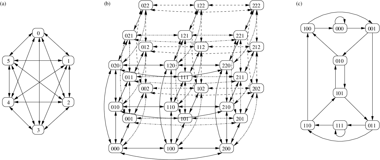
A rewriting code for flash memories can be formally defined as follows. Note that in the flash-memory model, $n$ cells of $q$ levels are used. The definition below can be easily extended to other constrained memory models.

Definition 3

. (Rewriting Code)

A rewriting code has a decoding function $F_{d}$ and an update function $F_{u}$ . The decoding function

F_{d}:\{0,1,\dots,q-1\}^{n}\to V_{\mathcal{D}}

means that the cell state $s\in\{0,1,\dots,q-1\}^{n}$ represents the data $F_{d}(s)\in V_{\mathcal{D}}$ . The update function (which represents a rewrite operation),

F_{u}:\{0,1,\dots,q-1\}^{n}\times V_{\mathcal{D}}\to\{0,1,\dots,q-1\}^{n},

means that if the current cell state is $s\in\{0,1,\dots,q-1\}^{n}$ and the rewrite changes the data to $v\in V_{\mathcal{D}}$ , then the rewriting code changes the cell state to $F_{u}(s,v)$ . All the following must hold:

1.

$(F_{d}(s),v)\in E_{\mathcal{D}}$ .
2.

The cell-state vector $F_{u}(s,v)$ is above $s$ .
3.

$F_{d}(F_{u}(s,v))=v$ .

Note that if $F_{d}(s)=v$ , we may set $F_{u}(s,v)=s$ , which corresponds to the case where we do not need to change the stored data. Throughout the paper we do not consider such a case as a rewrite operation. $\Box$

A sequence of rewrites is a sequence $(v_{0},v_{1},v_{2}\dots)$ such that the $i$ -th rewrite changes the stored data from $v_{i-1}$ to $v_{i}$ . Given a rewriting code $\mathcal{C}$ , we denote by $t(\mathcal{C})$ the maximal number of rewrites that $\mathcal{C}$ guarantees to support for all rewrite sequences. Thus, $t(\mathcal{C})$ is a worst-case performance measure of the code. The code $\mathcal{C}$ is said to be optimal if $t(\mathcal{C})$ is maximized. In addition to this definition, if a probabilistic model for rewrite sequences is considered, the expected rewriting performance can be defined accordingly.

In this paper, we study generalized rewriting for the flash-memory model. We present a novel rewriting code, called the trajectory code, which is provably asymptotically optimal (up to constant factors) for a very wide range of scenarios. The idea of the code is to trace the changes of data in the data graph $\mathcal{D}$ . The trajectory code includes WOM codes, floating codes, and buffer codes as special cases.

We also study randomized rewriting codes and design codes that are optimized for the expected rewriting performance (namely, the expected number of rewrites the code supports). A rewriting code is called robust if its expected rewriting performance is asymptotically optimal for all rewrite sequences. We present a randomized code construction that is robust.

Both our codes for general rewriting and our robust code are optimal up to constant factors (factors independent of the problem parameters). Namely, for a constant $r\leqslant 1$ , we present codes $\mathcal{C}$ for which $t(\mathcal{C})$ is at least $r$ times that of the optimal code. We would like to note that, for our robust code, the constant involved is arbitrarily close to $1$ .

The rest of the paper is organized as follows. In Section II, we review the related results on rewriting codes, and compare them to the results derived in this paper. In Section III, a new rewriting code for the generalized rewriting model, the trajectory code, is presented and its optimality is proved. In Section IV, robust codes optimized for expected rewriting performance are presented. In Section V, the concluding remarks are presented.

II Overview of Related Results

There has been a history of distinguished theoretical study on constrained memories. It includes the original work by Kuznetsov and Tsybakov on coding for defective memories [18]. Further developments on defective memories include [11, 9]. The write-once memory (WOM) [23], write-unidirectional memory (WUM) [25, 24, 26], and write-efficient memory [1, 8], are also special instances of constrained memories. Among them, WOM is the most related to the flash-memory model studied in this paper.

Write-once memory (WOM) was studied by Rivest and Shamir in their original work [23]. In a WOM, a cell’s state can change from 0 to 1 but not from 1 to 0. This model was later generalized with more cell states in [5, 7]. The objective of WOM codes is to maximize the number of times that the stored data can be rewritten. A number of very interesting WOM code constructions have been presented over the years, including the tabular codes, linear codes, and others in [23], the linear codes in [5], the codes constructed using projective geometries [20], and the coset coding in [4]. Profound results on the capacity of WOM have been presented in [7, 10, 23, 27]. Furthermore, error-correcting WOM codes have been studied in [34]. In all the above works, the rewriting model assumes no constraints on the data, namely, the data graph $\mathcal{D}$ is a complete graph.

With the increasing importance of flash memories, the flash-memory model was proposed and studied recently in [2, 12, 13]. The rewriting schemes include floating codes [12, 13, 14, 15] and buffer codes [2, 14]. Both types of codes use the joint coding of multiple variables for better rewriting capability. Their data graphs $\mathcal{D}$ are generalized hypercubes and de Bruijn graphs, respectively. Multiple floating codes have been presented, including the code constructions in [13, 15], the flash codes in [19, 33], and the constructions based on Gray codes in [6]. The floating codes in [6] were optimized for the expected rewriting performance. The study of WOM codes – with new applications to flash memories – is also continued, with a number of improved code constructions [16, 28, 29, 30, 31].

Compared to existing codes, the codes in this paper not only work for a more general rewriting model, but also provide efficiently encodable and decodable asymptotically-optimal performance for a wider range of cases. This can be seen clearly from Table I, where the asymptotically-optimal codes are summarized. We explain some of the parameters in Table I here. For the WOM code, a variable of alphabet size $\ell$ is stored. For the floating code and the buffer code, $k$ variables of alphabet size $\ell$ are stored. For rewriting codes using the generalized rewriting model, $L$ is the size of the data graph. For all the codes, $n$ cells are used to store the data. It can be seen that this paper substantially expands the known results on rewriting codes.

TABLE I: A summary of the rewriting codes with asymptotically optimal performance (up to constant factors). Here

n,k,\ell,L

are as defined in Section I and Section II.

Type	Asymptotic optimality	ref.
WOM code ( $\mathcal{D}$ is a complete graph)	$t(\mathcal{C})$ is asymptotically optimal	[23]
WOM code ( $\mathcal{D}$ is a complete graph)	$t(\mathcal{C})$ is asymptotically optimal when $\ell=\Theta(1)$	[5]
Floating code ( $\mathcal{D}$ is a hypercube)	$t(\mathcal{C})$ is asymptotically optimal when $k=\Theta(1)$ and $\ell=\Theta(1)$	[13] [15]
Floating code ( $\mathcal{D}$ is a hypercube)	$t(\mathcal{C})$ is asymptotically optimal when $n=\Omega(k\log k)$ and $\ell=\Theta(1)$	[13] [15]
Floating code ( $\mathcal{D}$ is a hypercube)	$t(\mathcal{C})$ is asymptotically optimal when $n=\Omega(k^{2})$ and $\ell=\Theta(1)$	[33]
Buffer code ( $\mathcal{D}$ is a de Bruijn graph)	$t(\mathcal{C})$ is asymptotically optimal when $n=\Omega(k)$ and $\ell=\Theta(1)$	[2] [32]
Floating code ( $\mathcal{D}$ is a hypercube)	codes designed for random rewriting sequences when $k=\Theta(1)$ and $\ell=2$	[6]
WOM code ( $\mathcal{D}$ is a complete graph)	$t(\mathcal{C})$ is asymptotically optimal	this paper
Rewriting code for the generalized	For any $\Delta$ , $t(\mathcal{C})$ is asymptotically optimal when $n=\Omega(\log L)$	this paper
rewriting model ( $\mathcal{D}$ has maximum out-
degree $\Delta$ .)
Robust coding	Asymptotically optimal (with constant $1-\varepsilon$ ) when $nq=\Omega(L\log L)$	this paper

III Trajectory Code

We use the flash-memory model of Definition 1 and the generalized rewriting model of Definition 2 in the rest of this paper. We first present a novel code construction, the trajectory code, then show its performance is asymptotically optimal.

III-A Trajectory Code Outline

Let $n_{0},n_{1},n_{2},\dots,n_{d}$ be $d+1$ positive integers and let

n=\sum_{i=0}^{d}n_{i},

where $n$ denotes the number of flash-memory cells, each of $q$ levels. We partition the $n$ cells into $d+1$ groups, each with $n_{0},n_{1},\dots,n_{d}$ cells, respectively. We call them registers $S_{0},S_{1},\dots,S_{d}$ , respectively.

Our encoding uses the following basic scheme: we start by using register $S_{0}$ , called the anchor, to record the value of the initial data $v_{0}\in V_{\mathcal{D}}$ .

For the next $d$ rewrite operations we use a differential scheme: denote by $v_{1},\dots,v_{d}\in V_{\mathcal{D}}$ the next $d$ values of the rewritten data. In the $i$ -th rewrite, $1\leqslant i\leqslant d$ , we store in register $S_{i}$ the identity of the edge $(v_{i-1},v_{i})\in E_{\mathcal{D}}$ . We do not require a unique label for all edges globally, but rather require that locally, for each vertex in $V_{\mathcal{D}}$ , its out-going edges have unique labels from $\left\{1,\dots,\Delta\right\}$ , where $\Delta$ denotes the maximal out-degree in the data graph $\mathcal{D}$ .

Intuitively, the first $d$ rewrite operations are achieved by encoding the trajectory taken by the input sequence starting with the anchor data. After $d$ such rewrites, we repeat the process by rewriting the next input from $V_{\mathcal{D}}$ in the anchor $S_{0}$ , and then continuing with $d$ edge labels in $S_{1},\dots,S_{d}$ .

Let us assume a sequence of $s$ rewrites have been stored thus far. To decode the last stored value, all we need to know is $s\mod(d+1)$ . This is easily achieved by using $\left\lceil t/q\right\rceil$ more cells (not specified in the previous $d+1$ registers), where $t$ is the total number of rewrite operations we would like to guarantee. For these $\left\lceil t/q\right\rceil$ cells we employ a simple encoding scheme: in every rewrite operation we arbitrarily choose one of those cells and raise its level by one. Thus, the total level in these cells equals $s$ .

The decoding process takes the value of the anchor $S_{0}$ and then follows $(s-1)\mod(d+1)$ edges which are read consecutively from $S_{1},S_{2},\dots$ . Notice that this scheme is appealing in cases where the maximum out-degree of $\mathcal{D}$ is significantly lower than the size of the state space $|V_{\mathcal{D}}|$ .

Note that for $i=0,1,\dots,d$ , each register $S_{i}$ can be seen as a smaller rewriting code whose data graph is a complete graph of either $L$ vertices (for $S_{0}$ ) or $\Delta$ vertices (for $S_{1},\dots,S_{d}$ ). We let $d=0$ if $\mathcal{D}$ is a complete graph, and describe how to set $d$ when $\mathcal{D}$ is not a complete graph in section III-C. The encoding used by each register is described in the next section.

III-B Analysis for a Complete Data Graph

In this section we present an efficiently encodable and decodable code that enables us to store and rewrite symbols from an input alphabet $V_{\mathcal{D}}$ of size $L\geqslant 2$ , when $\mathcal{D}$ is a complete graph. The information is stored in $n$ flash-memory cells of $q$ levels each.

We first state a scheme that allows approximately $nq/8$ rewrites in the case in which $2\leqslant L\leqslant n$ . We then extend it to hold for general $L$ and $n$ . We present the quality of our code constructions (namely the number of possible rewrites they perform) using asymptotic notation: $O(\cdot)$ , $\Omega(\cdot)$ , $\Theta(\cdot)$ , $o(\cdot)$ , and $\omega(\cdot)$ (where in all cases $n$ is considered to be the asymptotic variable that tends to infinity).

III-B1 The case of $2\leqslant L\leqslant n$

In this section we present a code for small values of $L$ . The code we present is essentially the one presented in [23].

Construction 1

. Let $2\leqslant L\leqslant n$ . This construction produces an efficiently encodable and decodable rewriting code $\mathcal{C}$ for a complete data graph $\mathcal{D}$ with $L$ states, and flash memory with $n$ cells with $q$ levels each.

Let us first assume $n=L$ . Denote the $n$ cell levels by $\vec{c}=(c_{0},c_{1},\dots,c_{L-1})$ , where $c_{i}\in\{0,1,\dots,q-1\}$ is the level of the $i$ -th cell for $i=0,1,\dots,L-1$ . Denote the alphabet of the data by $V_{\mathcal{D}}=\{0,1,\dots,L-1\}$ . We first use only cell levels 0 and 1, and the data stored in the cells is

\sum_{i=0}^{L-1}ic_{i}\pmod{L}.

With each rewrite, we increase the minimum number of cell levels from 0 to 1 so that the new cell state represents the new data. (Clearly, $c_{0}$ remains untouched as 0.) When the code can no longer support rewriting, we increase all cells (including $c_{0}$ ) from 0 to 1, and start using cell levels 1 and 2 to store data in the same way as above, except that the data stored in the cells uses the formula

\sum_{i=0}^{L-1}i(c_{i}-1)\pmod{L}.

This process is repeated $q-1$ times in total. The general decoding function is therefore defined as

F_{d}(\vec{c})=\sum_{i=0}^{L-1}i(c_{i}-c_{0})\pmod{L}.

We now extend the above code to $n\geqslant L$ cells. We divide the $n$ cells into $b=\left\lfloor n/L\right\rfloor$ groups of size $L$ (some cells may remain unused). We first apply the code above to the first group of $L$ cells, then to the second group, and so on. $\Box$

Theorem 4

. Let $2\leqslant L\leqslant n$ . The number of rewrites the code $\mathcal{C}$ of Construction 1 guarantees is lower bounded by

t(\mathcal{C})\geqslant n(q-1)/8=\Omega(nq).

Proof:

First assume $n=L$ . When cell levels $j-1$ and $j$ are used to store data (for $j=1,\dots,q-1$ ), by the analysis in [23], even if only one or two cells increase their levels with each rewrite, at least $(L+4)/4$ rewrites can be supported. So the $L$ cells can support at least

t(\mathcal{C})\geqslant\frac{(L+4)(q-1)}{4}=\Omega(nq)

rewrites. Now let $n\geqslant L$ . When $b=\left\lfloor n/L\right\rfloor$ , it is easy to see that $bL\geqslant n/2$ . The $b$ groups of cells can guarantee

t(\mathcal{C})\geqslant\frac{b(L+4)(q-1)}{4}\geqslant\frac{n(q-1)}{8}=\Omega(nq)

rewrites.

III-B2 The Case of Large $L$

We now consider the setting in which $L$ is larger than $n$ . The rewriting code we present reduces the general case to that of the case $n=L$ studied above. The majority of our analysis addresses the case in which $n<L\leqslant 2^{n/16}$ . We start, however, by first considering the simple case in which $2^{n/16}\leqslant L\leqslant q^{n}$ . Notice that if $L$ is greater than $q^{n}$ then we cannot guarantee even a single rewrite.

Construction 2

. Let $c\in[2^{1/16},q]$ , and let $L=c^{n}$ . This construction produces an efficiently encodable and decodable rewriting code $\mathcal{C}$ for a complete data graph $\mathcal{D}$ with $L$ states, and flash memory with $n$ cells with $q$ levels each.

Denote the $n$ cell levels by $\vec{c}=(c_{0},c_{1},\dots,c_{n-1})$ , where $c_{i}\in\{0,1,\dots,q-1\}$ is the level of the $i$ -th cell for $i=0,1,\dots,n-1$ . Denote the alphabet of data by $V_{\mathcal{D}}=\{0,1,\dots,L-1\}$ . For the initial (re)write we use only cell levels 0 to $\left\lceil c\right\rceil-1$ , and the data stored in the cells is

\sum_{i=0}^{n-1}c_{i}\left\lceil c\right\rceil^{i}\pmod{L}.

With the next rewrite, we use the cell levels $\left\lceil c\right\rceil$ to $2\left\lceil c\right\rceil-1$ and the data stored in the cells is now

\sum_{i=0}^{n-1}(c_{i}-\left\lceil c\right\rceil)\left\lceil c\right\rceil^{i}\pmod{L}

and so on. In general,

F_{d}(\vec{c})=\sum_{i=0}^{n-1}(c_{i}\bmod\left\lceil c\right\rceil)\left\lceil c\right\rceil^{i}\pmod{L}.

and with each rewrite we represent $v\in V_{\mathcal{D}}$ by its $n$ -character representation over an alphabet of size $\left\lceil c\right\rceil$ . $\Box$

The following theorem is immediate.

Theorem 5

. Let $c\in[2^{1/16},q]$ . If $L=c^{n}$ then the code $\mathcal{C}$ of Construction 2 guarantees $t(\mathcal{C})\geqslant q/\left\lceil c\right\rceil=\Omega(q/c)$ .

We now address the case $n<L\leqslant 2^{n/16}$ . Let $b$ be the smallest positive integer value that satisfies

\left\lfloor n/b\right\rfloor^{b}\geqslant L.

Claim 6

. For $n\leqslant L\leqslant 2^{n/16}$ , it holds that

b\leqslant\frac{2\log{L}}{\log{(n/\log{L})}}.

Proof:

Let $b=\frac{2\log{L}}{\log{(n/\log{L})}}$ . Notice that

\left\lfloor n/b\right\rfloor\geqslant\frac{n\log{(n/\log{L})}}{4\log{L}}.

Thus,

	$\displaystyle\log{\left\lfloor n/b\right\rfloor^{b}}$	$\displaystyle=b\log{\left\lfloor n/b\right\rfloor}$
		$\displaystyle\geqslant\frac{2\log{L}}{\log{(n/\log{L})}}\log\left(\frac{n\log{(n/\log{L})}}{4\log{L}}\right)$
		$\displaystyle\geqslant\frac{2\log{L}}{\log{(n/\log{L})}}\log\left(\frac{n}{4\log{L}}\right)$
		$\displaystyle\geqslant\frac{2\log{L}}{\log{(n/\log{L})}}\log\left(\sqrt{\frac{n}{\log{L}}}\right)=\log{L}$

We used the fact that $L\leqslant 2^{n/16}$ to establish the inequality $\frac{n}{4\log{L}}\geqslant\sqrt{\frac{n}{\log{L}}}$ used in the last step above.

Construction 3

. Let $n<L\leqslant 2^{n/16}$ . This construction produces an efficiently encodable and decodable rewriting code $\mathcal{C}$ for a complete data graph $\mathcal{D}$ with $L$ states, and flash memory with $n$ cells with $q$ levels each.

For $i=1,2,\dots,b$ , let $v_{i}$ be a symbol from an alphabet of size

\left\lfloor n/b\right\rfloor\geqslant L^{1/b}.

We may represent any symbol $v\in V_{\mathcal{D}}$ as a vector of symbols $(v_{1},v_{2},\dots,v_{b})$ .

Partition the $n$ flash-memory cells into $b$ groups, each with $\left\lfloor n/b\right\rfloor$ cells (some cells may remain unused). Encoding the symbol $v$ into $n$ cells is equivalent to the encoding of each $v_{i}$ into the corresponding group of $\left\lfloor n/b\right\rfloor$ cells. As the alphabet size of each $v_{i}$ equals the number of cells it is to be encoded into, we can use Construction 1 to store $v_{i}$ . $\Box$

Example 7

. Let $n=16$ , $q=4$ , $L=56$ , and the data graph $\mathcal{D}$ be a complete graph. We design a rewriting code for these parameters with the method of Construction 3.

Let $b=2$ , and we divide the $n=16$ cells evenly into $b=2$ groups. Let $\vec{c}=(c_{0},c_{1},\dots,c_{7})$ denote the cell levels of the first cell group, and let $\vec{c}^{\prime}=(c_{0}^{\prime},c_{1}^{\prime},\dots,c_{7}^{\prime})$ denote the cell levels of the second cell group.

Let $v\in\{0,1,\dots,L-1\}=\{0,1,\dots,55\}$ denote the value of the stored data. Let $v_{1}$ and $v_{2}$ be two symbols of alphabet size $8$ . We can represent $v$ by the pair $(v_{1},v_{2})$ as follows:

v_{1}=\left\lfloor v/8\right\rfloor\qquad\qquad v_{2}=v\bmod 8.

We store $v_{1}$ in the first cell group using the decoding function

v_{1}=\sum_{i=0}^{7}i(c_{i}-c_{0})\pmod{8},

and store $v_{2}$ in the second cell group using the decoding function

v_{2}=\sum_{i=0}^{7}i(c_{i}^{\prime}-c_{0}^{\prime})\pmod{8}.

Reconstructing $v$ from $(v_{1},v_{2})$ is done by $v=8v_{1}+v_{2}$ . Thus, if the data, $v$ , changes as

0\to 23\to 45\to 6\to 27\to 12,

the symbol pair $(v_{1},v_{2})$ will change as

(0,0)\to(2,7)\to(5,5)\to(0,6)\to(3,3)\to(1,4),

and the cell levels $(\vec{c},\vec{c}^{\prime})=((c_{0},c_{1},\dots,c_{7}),(c_{0}^{\prime},c_{1}^{\prime},\dots,c_{7}^{\prime}))$ will change as

	$\displaystyle((0,0,0,0,0,0,0,0),(0,0,0,0,0,0,0,0))$
	$\displaystyle\downarrow$
	$\displaystyle((0,0,1,0,0,0,0,0),(0,0,0,0,0,0,0,1))$
	$\displaystyle\downarrow$
	$\displaystyle((0,0,1,1,0,0,0,0),(0,0,0,0,0,0,1,1))$
	$\displaystyle\downarrow$
	$\displaystyle((0,0,1,1,1,0,0,1),(0,1,0,0,0,0,1,1))$
	$\displaystyle\downarrow$
	$\displaystyle((0,0,1,1,1,1,1,1),(0,1,0,0,0,1,1,1))$
	$\displaystyle\downarrow$
	$\displaystyle((1,2,1,1,1,1,1,1),(0,1,1,1,1,1,1,1))$

A careful reader will have observed that the parameters here actually do not satisfy the condition $n<L\leqslant 2^{n/16}$ . Indeed, the condition $n<L\leqslant 2^{n/16}$ is chosen only for the analysis of the asymptotic performance. The rewriting code of Construction 3 can be used for more general parameter settings. $\Box$

Theorem 8

. Let $n\leqslant L\leqslant 2^{n/16}$ . The number of rewrites the code $\mathcal{C}$ of Construction 3 guarantees is lower bounded by

t(\mathcal{C})\geqslant\frac{n(q-1)\log{(n/\log{L})}}{16\log{L}}=\Omega\left(\frac{nq\log{(n/\log{L})}}{\log{L}}\right).

Proof:

Using Construction 3, the number of rewrites possible is bounded by the number of rewrites possible for each of the $b$ cell groups. By Theorem 4 and Claim 6, this is at least

	$\displaystyle\left\lfloor\frac{n}{b}\right\rfloor\cdot\frac{q-1}{8}$	$\displaystyle\geqslant\left(\frac{n\log{(n/\log{L})}}{2\log L}-1\right)\frac{q-1}{8}$
		$\displaystyle=\Omega\left(\frac{nq\log{(n/\log{L})}}{\log{L}}\right).$

III-C Analysis for a Bounded-Out-Degree Data Graph

We now return to the outline of the trajectory code from Section III-A, and apply it in full detail using the codes from Section III-B to the case of data graphs $\mathcal{D}$ with upper bounded out-degree $\Delta$ . We refer to such graphs as $\Delta$ -restricted. To simplify our presentation, in the theorems below we will again use the asymptotic notation freely; however, as opposed to the previous section we will no longer state or make an attempt to optimize the constants involved in our calculations. We assume that $n\leqslant L$ , since for $L\leqslant n$ , Construction 1 can be used to obtain optimal codes (up to constant factors). In this section we study the case $L\leqslant 2^{n/16}$ . We do not address the case of larger $L$ , as its analysis, although based on similar ideas, becomes rather tedious and overly lengthy.

Using the notation of Section III-A, to realize the trajectory code we need to specify the sizes $n_{i}$ and the value of $d$ . We consider two cases: the case in which $\Delta$ is small compared to $n$ , and the case in which $\Delta$ is large.

The following construction is for the case in which $\Delta$ is small compared to $n$ .

Construction 4

. Let

\Delta\leqslant\left\lfloor\frac{n\log{(n/\log{L})}}{2\log{L}}\right\rfloor.

We build an efficiently encodable and decodable rewriting code $\mathcal{C}$ for any $\Delta$ -restricted data graph $\mathcal{D}$ with $L$ vertices and $n$ flash-memory cells of $q$ levels as follows. For the trajectory code, let

d=\left\lfloor\log L/\log{(n/\log{L})}\right\rfloor=\Theta(\log L/\log{(n/\log{L})}).

Set the size of the $d+1$ registers to

n_{0}=\left\lfloor n/2\right\rfloor

and

n_{i}=\left\lfloor n/(2d)\right\rfloor\geqslant\Delta

for $i=1,2,\dots,d$ . (We obviously have $\sum_{i=0}^{d}n_{i}\leqslant n$ .)

The update and decoding functions of the trajectory code $\mathcal{C}$ are defined as follows. We use the encoding scheme specified in Construction 3 to store in the $n_{0}$ cells of the register $S_{0}$ an “anchor” (i.e., a vertex) of $\mathcal{D}$ , which is a symbol in the alphabet $V_{\mathcal{D}}=\{0,1,\dots,L-1\}$ .

For $i=1,2,\dots,d$ , we use the encoding scheme specified in Construction 1 to store in the $n_{i}$ cells of the register $S_{i}$ an “edge” of $\mathcal{D}$ , which is a symbol in the alphabet $\{0,1,\dots,\Delta-1\}$ . Notice that the latter is possible because $n_{i}\geqslant\Delta$ for $i=1,\dots d$ . $\Box$

Recall that the anchor and the edges stored in $S_{0},S_{1},S_{2},\dots$ show how the data changes its value with rewrites. That is, they show the trace of the changing data in the data graph $\mathcal{D}$ . Every $d+1$ rewrites change the data stored in the register $S_{i}$ exactly once, for $i=0,1,\dots,d$ . After every $d+1$ rewrites, the next rewrite resets the anchor’s value in $S_{0}$ , and the same rewriting process starts again.

Suppose that the rewrites change the stored data as $v_{0}\to\cdots\to v_{i}\to v_{i+1}\to\cdots$ . Then with the rewriting code of Construction 4, the data stored in the register $S_{0}$ changes as $v_{0}\to v_{d+1}\to v_{2(d+1)}\to v_{3(d+1)}\to\cdots$ . For $i=1,2,\dots,d$ , the data stored in the register $S_{i}$ changes as $(v_{i-1},v_{i})\to(v_{i-1+(d+1)},v_{i+(d+1)})\to(v_{i-1+2(d+1)},v_{i+2(d+1)})\to(v_{i-1+3(d+1)},v_{i+3(d+1)})\to\cdots$ Here every edge $(v_{j-1},v_{j})\in E_{\mathcal{D}}$ is locally labeled by the alphabet $\{0,1,\dots,\Delta-1\}$ .

Theorem 9

. Let $L\leqslant 2^{n/16}$ and $\Delta\leqslant\left\lfloor\frac{n\log{(n/\log{L})}}{2\log{L}}\right\rfloor$ . The number of rewrites the code $\mathcal{C}$ of Construction 4 guarantees is

t(\mathcal{C})=\Omega(nq)

Proof:

By Theorems 8 and 4, the lower bound on the number of rewrites possible in $S_{0}$ is equal (up to constant factors) to that of $S_{i}$ ( $i\geqslant 1$ ):

	$\displaystyle\Omega\left(\frac{n_{0}q\log{(n_{0}/\log{L})}}{\log{L}}\right)$	$\displaystyle=\Omega\left(\frac{nq\log{(n/\log{L})}}{\log{L}}\right)$
		$\displaystyle=\Omega\left(\frac{nq}{d}\right)=\Omega\left(n_{i}q\right).$

Thus, the total number of rewrites in the scheme outlined in Section III-A is lower bounded by $d+1$ times the bound for each register $S_{i}$ , and so $t(\mathcal{C})=\Omega(nq)$ .

Example 10

. Consider floating codes, where $k$ variables of alphabet size $\ell$ are stored in $n$ cells of $q$ levels. When Construction 4 is used to build the floating code, we get $L=\ell^{k}$ and $\Delta=k(\ell-1)$ . So if $k(\ell-1)\leqslant\left\lfloor\frac{n\log{(n/(k\log{\ell}))}}{2k\log\ell}\right\rfloor$ , the code can guarantee $t(\mathcal{C})=\Omega(nq)$ rewrites, which is asymptotically optimal. $\Box$

The next construction is for the case in which $\Delta$ is large compared to $n$ .

Construction 5

. Let $L\leqslant 2^{n/16}$ and let

\left\lfloor\frac{n\log{(n/\log{L})}}{2\log{L}}\right\rfloor\leqslant\Delta\leqslant L-1.

d=\left\lfloor\log L/\log{\Delta}\right\rfloor=\Theta(\log L/\log{\Delta}).

Set the size of the registers to

n_{0}=\left\lfloor n/2\right\rfloor

and

n_{i}=\left\lfloor n/(2d)\right\rfloor

for $i=1,2,\dots,d$ .

The update and decoding functions of the trajectory code $\mathcal{C}$ are defined as follows: use the encoding scheme specified in Construction 3 to store an “anchor” in $S_{0}$ and store an “edge” in $S_{i}$ , for $i=1,2,\dots,d$ . (The remaining details are the same as Construction 4.) $\Box$

Theorem 11

. Let $L\leqslant 2^{n/16}$ . Let $\left\lfloor\frac{n\log{(n/\log{L})}}{2\log{L}}\right\rfloor\leqslant\Delta\leqslant L-1$ . The number of rewrites the code $\mathcal{C}$ of Construction 5 guarantees is lower bounded by

t(\mathcal{C})=\Omega\left(\frac{nq\log{(n/\log{L})}}{\log{\Delta}}\right).

Proof:

By Theorem 8, the number of rewrites supported in $S_{0}$ is lower bounded by

\Omega\left(\frac{n_{0}q\log{(n_{0}/\log{L})}}{\log{L}}\right)=\Omega\left(\frac{nq\log{(n/\log{L})}}{\log{L}}\right)

Similarly, for $i=1,2,\dots,d$ , the number of rewrites supported in $S_{i}$ is lower bounded by

	$\displaystyle\Omega\left(\frac{n_{i}q\log{(n_{i}/\log{\Delta})}}{\log{\Delta}}\right)$	$\displaystyle=\Omega\left(\frac{nq\log{(n/\log{L})}}{d\log{\Delta}}\right)$
		$\displaystyle=\Omega\left(\frac{nq\log{(n/\log{L})}}{\log{L}}\right).$

Thus, as in Theorem 9, we conclude that the total number of rewrites in the scheme outlined in Section III-A is lower bounded by $d+1$ times the bound for each register $S_{i}$ , and so $t(\mathcal{C})=\Omega\left(\frac{nq\log{(n/\log{L})}}{\log{\Delta}}\right)$ .

III-D Optimality of the Code Constructions

We now prove upper bounds on the number of rewrites in general rewriting schemes, which match the lower bounds induced by our code constructions. They show that our code constructions are asymptotically optimal.

Theorem 12

. Any rewriting code $\mathcal{C}$ that stores symbols from some data graph $\mathcal{D}$ in $n$ flash-memory cells of $q$ levels supports at most

t(\mathcal{C})\leqslant n(q-1)=O(nq)

rewrites.

Proof:

The bound is trivial. In the best case, all cells are initialized at level $0$ , and every rewrite increases exactly one cell by exactly one level. Thus, the total number of rewrites is bounded by $n(q-1)=O(nq)$ as claimed.

Corollary 13

. The codes from Constructions 1 and 4 are asymptotically optimal.

For large values of $L$ , we can improve the upper bound. First, let $r$ denote the largest integer such that

\binom{r+n-1}{r}<L-1.

We need the following technical claim.

Claim 14

. Let $L\leqslant 2^{n/16}$ . For all $1\leqslant n<L-1$ , the following inequality

r\geqslant c\cdot\frac{\log{L}}{\log(n/\log{L})}

holds for a sufficiently small constant $c>0$ .

Proof:

First, it is easy to see that $r\in[1,n]$ . Now we may use the well-known bound for all $v\geqslant u\geqslant 1$ ,

\binom{v}{u}<\left(\frac{ev}{u}\right)^{u},

where $e$ is the base of the natural logarithm. Let $m=n/r$ . It follows that,

\binom{r+n-1}{r}\leqslant\binom{r+n}{r}\leqslant\binom{2n}{r}\leqslant\frac{2^{r}e^{r}n^{r}}{r^{r}}.

Hence,

\log\binom{r+n-1}{r}\leqslant r\log\left(\frac{2en}{r}\right)=\frac{n}{m}\log(2em).

Thus, it suffices to prove that

\frac{n}{m}\log(2em)<\log{(L-1)}.

We conclude via basic computations that if

m=c^{\prime}\cdot\frac{n\log{\left({n/\log{L}}\right)}}{\log{L}}

for a sufficiently large constant $c^{\prime}>0$ , then

\binom{r+n-1}{r}\leqslant L.

Theorem 15

. Let $L\leqslant 2^{n/16}$ . When $n<L-1$ , any rewriting code $\mathcal{C}$ that stores symbols from the complete data graph $\mathcal{D}$ in $n$ flash-memory cells of $q$ levels can guarantee at most

t(\mathcal{C})=O\left(\frac{nq\log{(n/\log{L})}}{\log{L}}\right)

rewrites.

Proof:

Let us examine some state $s$ of the $n$ flash-memory cells, currently storing some value $v\in V_{\mathcal{D}}$ , i.e., $F_{d}(s)=v$ . Having no constraint on the data graph, the next symbol we want to store may be any of the $L-1$ symbols $v^{\prime}\in V_{\mathcal{D}}$ , where $v^{\prime}\neq v$ .

If we allow ourselves $r$ operations of increasing a single cell level of the $n$ flash-memory cells by one (perhaps operating on the same cell more than once), we may reach at most

\binom{n+r-1}{r}

distinct new states. However, by our choice of $r$ , we have $\binom{n+r-1}{r}<L-1$ . So we need at least $r+1$ such operations to realize a rewrite in the worst case. Since we have a total of $n$ cells with $q$ levels each, the guaranteed number of rewrite operations is upper bounded by

t(\mathcal{C})\leqslant\frac{n(q-1)}{r+1}=O\left(\frac{nq\log{(n/\log{L})}}{\log L}\right).

Corollary 16

. The code from Construction 3 is asymptotically optimal.

Theorem 17

. Let $2^{n/16}\leqslant L=c^{n}\leqslant q^{n}$ . Any rewriting code $\mathcal{C}$ that stores symbols from the complete data graph $\mathcal{D}$ in $n$ flash-memory cells of $q$ levels can guarantee at most

t(\mathcal{C})=O\left(q/c\right)

rewrites.

Proof:

We follow the proof of Theorem 15. In this case we note that for $\binom{n+r-1}{r}$ to be at least of size $L=c^{n}$ we need $r=\Omega\left(nc\right)$ . The proof follows.

Corollary 18

. The code from Construction 2 is asymptotically optimal.

Theorem 19

. Let $L\leqslant 2^{n/16}$ . Let $\Delta>\left\lfloor\frac{n\log{(n/\log{L})}}{2\log{L}}\right\rfloor$ . There exist $\Delta$ -restricted data graphs $\mathcal{D}$ over a vertex set of size $L$ , such that any rewriting code $\mathcal{C}$ that stores symbols from the data graph $\mathcal{D}$ in $n$ flash-memory cells of $q$ levels can guarantee at most

t(\mathcal{C})=O\left(\frac{nq\log{(n/\log{L})}}{\log{\Delta}}\right)

rewrites.

Proof:

We start by showing that $\Delta$ -restricted graphs $\mathcal{D}$ with certain properties do not allow rewriting codes $\mathcal{C}$ that support more than $t(\mathcal{C})=O\left(\frac{nq\log{(n/\log{L})}}{\log{\Delta}}\right)$ rewrites. We then show that such graphs indeed exist. This will conclude our proof.

Let $\mathcal{D}$ be a $\Delta$ -restricted graph whose diameter $d$ is at most $O\left(\frac{\log{L}}{\log{\Delta}}\right)$ . Assuming the existence of such a graph $\mathcal{D}$ , consider (by contradiction) a rewriting code $\mathcal{C}$ for the $\Delta$ -restricted graph $\mathcal{D}$ that allows

t(\mathcal{C})=\omega\left(\frac{nq\log{(n/\log{L})}}{\log{\Delta}}\right)

rewrites. We use $\mathcal{C}$ to construct a rewriting code $\mathcal{C}^{\prime}$ for a new data graph $\mathcal{D}^{\prime}$ which has the same vertex set $V_{\mathcal{D}^{\prime}}=V_{\mathcal{D}}$ but is a complete graph. The code $\mathcal{C}^{\prime}$ will allow

t(\mathcal{C}^{\prime})=\omega\left(\frac{nq\log{(n/\log{L})}}{\log{L}}\right)

rewrites, a contradiction to Theorem 15. This will imply that our initial assumption regarding the quality of our rewriting code $\mathcal{C}$ is false.

The rewriting code $\mathcal{C}^{\prime}$ (defined by the decoding function $F^{\prime}_{d}$ and the update function $F^{\prime}_{u}$ ) is constructed by mimicking $\mathcal{C}$ (defined by the decoding function $F_{d}$ and the update function $F_{u}$ ). We start by setting $F^{\prime}_{d}=F_{d}$ . Next, let $s$ be some state of the flash cells. Denote $F_{d}(s)=F^{\prime}_{d}(s)=v_{0}\in V_{\mathcal{D}}$ . Consider a rewrite operation attempting to store a new value $v_{1}\in V_{\mathcal{D}}$ , where $v_{1}\neq v_{0}$ . There exists a path in $\mathcal{D}$ of length $d^{\prime}$ , where $d^{\prime}\leqslant d$ , from $v_{0}$ to $v_{1}$ , which we denote by

v_{0},u_{1},u_{2},\dots,u_{d^{\prime}-1},v_{1}.

We now define

F^{\prime}_{u}(s,v_{1})=F_{u}(F_{u}(\dots F_{u}(F_{u}(s,u_{1}),u_{2})\dots,u_{d^{\prime}-1}),v_{1}),

which simply states that to encode a new value $v_{1}$ we follow the steps taken by the code $\mathcal{C}$ on a short path from $v_{0}$ to $v_{1}$ in the data graph $\mathcal{D}$ .

As $\mathcal{C}$ guarantees $t(\mathcal{C})=\omega\left(\frac{nq\log{(n/\log{L})}}{\log{\Delta}}\right)$ rewrites, the code for $\mathcal{C}^{\prime}$ guarantees at least

t(\mathcal{C}^{\prime})=\omega\left(\frac{nq\log{(n/\log{L})}}{d\log{\Delta}}\right)=\omega\left(\frac{nq\log{(n/\log{L})}}{\log{L}}\right)

rewrites. Here we use the fact that $d=O\left(\frac{\log{L}}{\log{\Delta}}\right)$ .

What is left is to show the existence of data graphs $\mathcal{D}$ of maximum out-degree $\Delta$ whose diameter $d$ is at most $O\left(\frac{\log{L}}{\log{\Delta}}\right)$ . To obtain such a graph, one may simply take a rooted bi-directed tree of total degree $\Delta$ and corresponding depth $O\left(\frac{\log{L}}{\log{\Delta}}\right)$ .

Corollary 20

. For $L\leqslant 2^{n/16}$ , the code from Construction 5 is asymptotically optimal.

IV Robust Rewriting Codes

It addition to the worst-case rewriting performance, it is also interesting to design rewriting codes with good expected performance. In this section we consider the use of randomized codes to obtain good expected performance for all rewrite sequences.

Let $\vec{v}=(v_{1},v_{2},v_{3},\dots,v_{n(q-1)})$ denote a sequence of rewrites. That is, for $i=1,2,3,\dots,n(q-1)$ , the $i$ -th rewrite changes the data to the value $v_{i}\in\{0,1,\dots,L-1\}$ . By default, the original value of the data is $v_{0}=0$ , and since every rewrite changes the data, we require that for all $i\geqslant 1$ , $v_{i}\neq v_{i-1}$ . Also, as no more than $n(q-1)$ rewrites may be supported, the sequence $\vec{v}$ is limited to $n(q-1)$ elements.

Let $\mathcal{C}$ denote a rewriting code, which stores the data from an alphabet of size $L$ in $n$ cells of $q$ levels. The code $\mathcal{C}$ can only support a finite number of rewrites in the rewrite sequence $\vec{v}$ . We use $t(\mathcal{C}|\vec{v})$ to denote the number of rewrites in the rewrite sequence $\vec{v}$ that are supported by the code $\mathcal{C}$ . That is, if the code $\mathcal{C}$ can support the rewrites $v_{1},v_{2},\dots,$ up to $v_{k}$ , then $t(\mathcal{C}|\vec{v})=k$ .

Let $V$ denote the set of all possible rewrite sequences. If we are interested in the number of rewrites that a code $\mathcal{C}$ guarantees in the worst case, $t(\mathcal{C})$ , then we can see that

t(\mathcal{C})=\min_{\vec{v}\in V}t(\mathcal{C}|\vec{v}).

In this section, we are interested in the expected number of rewrites that a code $\mathcal{C}$ can support under random coding. Let $\mathcal{Q}$ be some distribution over rewriting codes and let $\mathcal{C}_{\mathcal{Q}}$ be a randomized code (namely, a random variable) with distribution $\mathcal{Q}$ . Let $\E(x)$ denote the expected value of a random variable $x$ . We define the expected performance of the randomized rewriting code $\mathcal{C}_{\mathcal{Q}}$ to be

\E_{\mathcal{C}_{\mathcal{Q}}}=\min_{\vec{v}\in V}\E(t(\mathcal{C}_{\mathcal{Q}}|\vec{v})).

Our objective is to maximize $\E_{\mathcal{C}_{\mathcal{Q}}}$ . Namely, to construct a distribution $\mathcal{Q}$ such that for all $\vec{v}$ , $\mathcal{C}_{\mathcal{Q}}$ will allow many rewrites in expectation. A code $\mathcal{C}_{\mathcal{Q}}$ whose $\E_{\mathcal{C}_{\mathcal{Q}}}$ is asymptotically optimal is called a robust code. For any constant $\varepsilon>0$ , in this section we will present a randomized code with $\E_{\mathcal{C}_{\mathcal{Q}}}\geqslant(1-\varepsilon)(q-1)n$ (clearly, the code is robust).

IV-A Code Construction

We first present our code construction, analyze its properties and define some useful terms. We then turn to show that it is indeed robust.

Let $(c_{1},c_{1},\dots,c_{n})$ denote the $n$ cell levels, where for $i=1,2,\dots,n$ , $c_{i}\in\{0,1,\dots,q-1\}$ is the $i$ -th cell’s level. Given a cell state $\vec{c}=(c_{1},c_{2},\dots,c_{n})$ , we define its weight, denoted by $w(\vec{c})$ , as

w(\vec{c})=\sum_{i=1}^{n}c_{i}.

Clearly, $0\leqslant w(\vec{c})\leqslant(q-1)n$ . Given the decoding function, $F_{d}:\{0,1,\dots,q-1\}^{n}\to\{0,1,\dots,L-1\}$ , of a rewriting code, the cell state $\vec{c}$ represents the data $F_{d}(\vec{c})$ .

Construction 6

. For all $i=0,1,\dots,n(q-1)-1$ and $j=1,2,\dots,n$ , let $\theta_{i,j}$ and $a_{i}$ be parameters chosen from the set $\{0,1,\dots,L-1\}$ .

We define a rewriting code $\mathcal{C}$ as follows. Its decoding function is

F_{d}(\vec{c})=\left(\sum_{i=1}^{n}\theta_{w(\vec{c})-1,i}c_{i}+\sum_{i=0}^{w(\vec{c})-1}a_{i}\right)\bmod L.

By default, if $\vec{c}=(0,0,\dots,0)$ , then $F_{d}(\vec{c})=0$ . When rewriting the data, we take a greedy approach: For every rewrite, minimize the increase of the cell state’s weight. (If there is a tie between cell states of the same weight, break the tie arbitrarily.) $\Box$

For simplicity, we will omit the term “ $\bmod\ L$ ” in all computations below that consist of values of data. For example, the expression for $F_{d}$ in the above code construction will be simply written as

F_{d}(\vec{c})=\sum_{i=1}^{n}\theta_{w(\vec{c})-1,i}c_{i}+\sum_{i=0}^{w(\vec{c})-1}a_{i},

and $F_{d}(\vec{c})-F_{d}(\vec{c^{\prime}})$ will mean $(F_{d}(\vec{c})-F_{d}(\vec{c^{\prime}}))\bmod L$ .

Definition 21

. (Update Vector and Update Diversity)

Let $\vec{c}=(c_{1},c_{2},\dots,c_{n})$ be a cell state where for $i=1,2,\dots,n$ , $c_{i}\in\{0,1,\dots,q-2\}$ . For $i=1,2,\dots,n$ , we define $N_{i}(\vec{c})$ as

N_{i}(\vec{c})=(c_{1},\dots,c_{i-1},c_{i}+1,c_{i+1},\dots,c_{n})

and define $e_{i}(\vec{c})$ as

e_{i}(\vec{c})=F_{d}(N_{i}(\vec{c}))-F_{d}(\vec{c}).

We also define the update vector of $\vec{c}$ , denoted by $u(\vec{c})$ , as

u(\vec{c})=(e_{1}(\vec{c}),e_{2}(\vec{c}),\dots,e_{n}(\vec{c})),

and the update diversity of $\vec{c}$ as

\left|\left\{e_{1}(\vec{c}),e_{2}(\vec{c}),\dots,e_{n}(\vec{c})\right\}\right|.

$\Box$

The update diversity of a cell state $\vec{c}$ is at most $L$ . If it is $L$ , it means that when the current cell state is $\vec{c}$ , no matter what the next rewrite is, we only need to increase one cell’s level by one to realize the rewrite. Specifically, if the next rewrite changes the data from $F_{d}(\vec{c})$ to $v^{\prime}$ , we will change from $\vec{c}$ to $N_{i}(\vec{c})$ by increasing the $i$ -th cell’s level by one such that

e_{i}(\vec{c})=v^{\prime}-F_{d}(\vec{c}).

For good rewriting performance, it is beneficial to make the update diversity of cell states large.

Lemma 22

. Let $\vec{c}=(c_{1},c_{2},\dots,c_{n})$ be a cell state where for $i=1,2,\dots,n$ , $c_{i}\in\{0,1,\dots,q-2\}$ . With the rewriting code of Construction 6, the update diversity of $\vec{c}$ is

\left|\left\{\theta_{w(\vec{c}),i}~|~i=1,2,\dots,n\right\}\right|.

Proof:

For $i=1,2,\dots,n$ , we have

	$\displaystyle e_{i}(\vec{c})$	$\displaystyle=F_{d}(N_{i}(\vec{c}))-F_{d}(\vec{c})$
		$\displaystyle=\sum_{j=1}^{n}\theta_{w(\vec{c}),j}c_{j}+\theta_{w(\vec{c}),i}+\sum_{j=0}^{w(\vec{c})}a_{j}$
		$\displaystyle\phantom{=}-\sum_{j=1}^{n}\theta_{w(\vec{c})-1,j}c_{j}-\sum_{j=0}^{w(\vec{c})-1}a_{j}$
		$\displaystyle=\theta_{w(\vec{c}),i}+a_{w(\vec{c})}+\sum_{j=1}^{n}(\theta_{w(\vec{c}),j}-\theta_{w(\vec{c})-1,j})c_{j}$

Only the first term, $\theta_{w(\vec{c}),i}$ , depends on $i$ . Hence the update diversity of $\vec{c}$ is

\left|\left\{e_{i}(\vec{c})~|~i=1,2,\dots,n\right\}\right|=\left|\left\{\theta_{w(\vec{c}),i}~|~i=1,2,\dots,n\right\}\right|.

Therefore, to make the update diversity of cell states large, we can make $\theta_{w(\vec{c}),1},\theta_{w(\vec{c}),2},\dots,\theta_{w(\vec{c}),n}$ take as many different values as possible. A simple solution is to let $\theta_{w(\vec{c}),i}=i$ for $i=1,2,\dots,n$ .

IV-B Robustness

In the following, we present our code for $n\geqslant L$ . (The case of smaller $n$ can be dealt with using Construction 3.) The code uses randomness in the code construction to combat adversarial rewrite sequences. We then analyze the asymptotic optimality of the code for $nq\geqslant L\log{L}$ , and show that it optimizes the constant in the asymptotic performance to $1-\varepsilon$ .

For $i=1,2,\dots,L$ , we define

g_{i}=\left\{j~|~1\leqslant j\leqslant n,j\equiv i\pmod{L}\right\}.

For example, if $n=8,L=3$ , then $g_{1}=\left\{1,4,7\right\},g_{2}=\left\{2,5,8\right\},g_{3}=\left\{3,6\right\}$ . For $i=1,2,\dots,L$ , $\left|g_{i}\right|$ is either $\left\lfloor n/L\right\rfloor$ or $\left\lceil n/L\right\rceil$ . We define

h_{i}=\sum_{j\in g_{i}}c_{j},

where $c_{j}$ is the $j$ -th cell’s level. For $i=1,2,\dots,L$ , we have

h_{i}\in\{0,1,\dots,|g_{i}|(q-1)\}.

We consider $g_{i}$ as a super cell whose level is $h_{i}$ .

Construction 7

. (Robust Code)

For $i=0,1,\dots,n(q-1)-1$ , choose the parameter $a_{i}$ independently and uniformly randomly from the set $\left\{0,1,\dots,L-1\right\}$ .

We define a randomized rewriting code $\mathcal{C}_{\mathcal{Q}}$ by its decoding function

F_{d}(\vec{c})=\sum_{i=1}^{L}ih_{i}+\sum_{i=0}^{w(\vec{c})-1}a_{i}.

(1)

By default, if $\vec{c}=(0,0,\dots,0)$ , then $F_{d}(\vec{c})=0$ . When rewriting the data, we take the same greedy approach as in Construction 6. $\Box$

When we consider $g_{1},g_{2},\dots,g_{L}$ as $L$ “super cells” whose levels are $\vec{c^{\prime}}=(h_{1},h_{2},\dots,h_{L})$ , we have

w(\vec{c})=\sum_{i=1}^{n}c_{i}=\sum_{i=1}^{L}h_{i}=w(\vec{c^{\prime}}).

The code of Construction 7 may be seen as a rewriting code that stores the data of alphabet size $L$ in $L$ super cells, whose decoding function is (1). Each of the super cells has either $(q-1)\left\lfloor n/L\right\rfloor+1$ levels or $(q-1)\left\lceil n/L\right\rceil+1$ levels.

Lemma 23

u(\vec{c^{\prime}})=\left(1+a_{w(\vec{c^{\prime}})},2+a_{w(\vec{c^{\prime}})},\dots,L+a_{w(\vec{c^{\prime}})}\right),

and the update diversity of the super-cell state $\vec{c^{\prime}}$ is $L$ .

Proof:

For $i=1,2,\dots,L$ , $N_{i}(\vec{c^{\prime}})=(h_{1},\dots,h_{i-1},h_{i}+1,h_{i+1},\dots,h_{L})$ , so

e_{i}(\vec{c^{\prime}})=F_{d}(N_{i}(\vec{c^{\prime}}))-F_{d}(\vec{c^{\prime}})=i+a_{w(\vec{c^{\prime}})}

and we get the conclusions.

Therefore, if the current super-cell state is $\vec{c^{\prime}}=(h_{1},h_{2},\dots,h_{L})$ where for $i=1,2,\dots,L$ , $h_{i}\leqslant(q-1)\left\lfloor n/L\right\rfloor-1$ , for the next rewrite, we only need to increase one super-cell’s level by one (which is equivalent to increasing one flash-memory cell’s level by one).

Lemma 24

. Let $\vec{c^{\prime}}=(h_{1},h_{2},\dots,h_{L})$ be a super-cell state where for $i=1,2,\dots,L$ , $h_{i}\leqslant(q-1)\left\lfloor n/L\right\rfloor-1$ . With the rewriting code of Construction 7, if $\vec{c^{\prime}}$ is the current super-cell state, then no matter which value the next rewrite changes the data to, the next rewrite will only increase one super cell’s level by one, and this super cell is uniformly randomly selected from the $L$ super cells. What is more, the selection of this super cell is independent of the past rewriting history (that is, independent of the super cells whose levels were chosen to increase for the previous rewrites).

Proof:

Let $\vec{c^{\prime}}$ be the current super-cell state, and assume the next rewrite changes the data to $v^{\prime}$ . By Lemma 23, we will realize the rewrite by increasing the $i$ -th super cell’s level by one such that $i+a_{w(\vec{c^{\prime}})}=v^{\prime}-F_{d}(\vec{c^{\prime}})$ . Since the parameter $a_{w(\vec{c^{\prime}})}$ is uniformly randomly chosen from the set $\{0,1,\dots,L-1\}$ , $i$ has a uniform random distribution over $\{1,2,\dots,L\}$ .

The same analysis holds for the previous rewrites. Note that with every rewrite, the weight of the super cells, $w(\vec{c^{\prime}})$ , increases. Since $a_{0},a_{1},\dots,a_{n(q-1)-1}$ are i.i.d. random variables, the selection of the super cell for this rewrite is independent of the selection for the previous rewrites.

The above lemma holds for every rewrite sequence. We now prove that the randomized rewriting code of Construction 7 is robust.

Theorem 25

. Let $\mathcal{C}_{\mathcal{Q}}$ be the randomized rewriting code of Construction 7. Let $\vec{v}=(v_{1},v_{2},v_{3},\dots)$ be any rewrite sequence. For any constant $\varepsilon>0$ there exists a constant $c=c(\varepsilon)>0$ such that if $nq\geqslant cL\log{L}$ , then

\E(t(\mathcal{C}_{\mathcal{Q}}|\vec{v}))\geqslant(1-\varepsilon)n(q-1),

and therefore $\mathcal{C}_{\mathcal{Q}}$ is a robust code.

Proof:

Consider $L$ bins such that the $i$ -th bin can hold $(q-1)\left|g_{i}\right|$ balls. We use $h_{i}$ to denote the number of balls in the $i$ -th bin. Note that every bin can contain at least $(q-1)\cdot\left\lfloor\frac{n}{L}\right\rfloor$ balls and at most $(q-1)\cdot\left\lceil\frac{n}{L}\right\rceil$ balls. By Lemma 24, before any bin is full, every rewrite throws a ball uniformly at random into one of the $L$ bins, independently of other rewrites. The rewriting process can always continue before any bin becomes full. Thus, the number of rewrites supported by the code $\mathcal{C}_{\mathcal{Q}}$ is at least the number of balls thrown to make at least one bin full.

Suppose that $n(q-1)-\alpha\sqrt{nq}$ balls are independently and uniformly at random thrown into $L$ bins, and there is no limit on the capacity of any bin. Here, we set $\alpha$ to be $c\sqrt{L\log{L}}$ for a sufficiently large constant $c$ . For $i=1,2,\dots,L$ , let $x_{i}$ denote the number of balls thrown into the $i$ -th bin. Clearly,

\E(x_{i})=\frac{n(q-1)}{L}-\frac{\alpha\sqrt{nq}}{L}.

By the Chernoff bound,

\pr\left(x_{i}\geqslant(q-1)\cdot\left\lfloor\frac{n}{L}\right\rfloor\right)\leqslant e^{-\Omega(\alpha^{2}/L)}.

By the union bound, the probability that one or more of the $L$ bins contain at least $(q-1)\cdot\left\lfloor\frac{n}{L}\right\rfloor$ balls is therefore upper bounded by $Le^{-\Omega(\alpha^{2}/L)}$ . By our setting of $\alpha$ we have $Le^{-\Omega(\alpha^{2}/L)}=2^{-\Omega(c^{2})}$ .

Therefore, when $n(q-1)-\alpha\sqrt{nq}$ balls are independently and uniformly at random thrown into $L$ bins, with high probability, all the $L$ bins have $(q-1)\cdot\left\lfloor\frac{n}{L}\right\rfloor-1$ or fewer balls. This suffices to conclude our assertion. Notice that our proof implies that with high probability (over $\mathcal{Q}$ ) the value of $t(\mathcal{C}_{\mathcal{Q}}|\vec{v})$ will be large. This stronger statement implies the asserted one in which we consider $E(t(\mathcal{C}_{\mathcal{Q}}|\vec{v}))$ .

V Concluding Remarks

In this paper, we presented a flexible rewriting model that generalizes known rewriting models, including those used by WOM codes, floating codes and buffer codes. We presented a novel code construction, the trajectory code, for this generalized rewriting model and proved that the code is asymptotically optimal for a very wide range of parameter settings, where the performance is measured by the number of rewrites supported by flash-memory cells in the worst case. We also studied the expected performance of rewriting codes, and presented a randomized robust code. It will be interesting to apply these new coding techniques to wider constrained-memory applications, and combine rewriting codes with error correction. These remain as our future research topics.

References

[1] R. Ahlswede and Z. Zhang, “On multiuser write-efficient memories,” in IEEE Transactions on Information Theory, vol. 40, no. 3, pp. 674–686, 1994.
[2] V. Bohossian, A. Jiang, and J. Bruck, “Buffer coding for asymmetric multi-level memory,” in Proc. IEEE International Symposium on Information Theory (ISIT), Nice, France, June 24-29, 2007, pp. 1186–1190.
[3] P. Cappelletti, C. Golla, P. Olivo, and E. Zanoni (Ed.), Flash memories. Kluwer Academic Publishers, 1999.
[4] G. D. Cohen, P. Godlewski, and F. Merkx, “Linear binary code for write-once memories,” in IEEE Transactions on Information Theory, vol. IT-32, no. 5, pp. 697–700, Sep. 1986.
[5] A. Fiat and A. Shamir, “Generalized “write-once” memories,” in IEEE Transactions on Information Theory, vol. IT-30, no. 3, pp. 470–480, May 1984.
[6] H. Finucane, Z. Liu, and M. Mitzenmacher, “Designing floating codes for expected performance,” in Proc. 46th Annual Allerton Conference on Communications, Control and Computing, Monticello, Illinois, USA, September 23-26, 2008, pp. 1389-1396.
[7] F. Fu and A. J. Han Vinck, “On the capacity of generalized write-once memory with state transitions described by an arbitrary directed acyclic graph,” in IEEE Transactions on Information Theory, vol. 45, no. 1, pp. 308–313, Jan. 1999.
[8] F. Fu and R. W. Yeung, “On the capacity and error-correcting codes of write-efficient memories,” in IEEE Transactions on Information Theory, vol. 46, no. 7, pp. 2299–2314, Nov. 2000.
[9] A. J. Han Vinck and A. V. Kuznetsov, “On the general defective channel with informed encoder and capacities of some constrained memories,” in IEEE Transactions on Information Theory, vol. 40, no. 6, pp. 1866–1871, 1994.
[10] C. D. Heegard, “On the capacity of permanent memory,” in IEEE Transactions on Information Theory, vol. IT-31, no. 1, pp. 34–42, Jan. 1985.
[11] C. D. Heegard and A. A. El-Gamal, “On the capacity of computer memory with defects,” in IEEE Transactions on Information Theory, vol. IT-29, no. 5, pp. 731–739, Sep. 1983.
[12] A. Jiang, “On the generalization of error-correcting WOM codes,” in Proc. IEEE International Symposium on Information Theory (ISIT), Nice, France, June 24-29, 2007, pp. 1391–1395.
[13] A. Jiang, V. Bohossian and J. Bruck, “Floating codes for joint information storage in write asymmetric memories,” in Proc. IEEE International Symposium on Information Theory (ISIT), Nice, France, June 24-29, 2007, pp. 1166–1170.
[14] A. Jiang, V. Bohossian and J. Bruck, “Rewriting codes for joint information storage in flash memories,” in IEEE Transactions on Information Theory, vol. 56, no. 10, pp. 5300–5313, October 2010.
[15] A. Jiang and J. Bruck, “Joint coding for flash memory storage,” in Proc. IEEE International Symposium on Information Theory (ISIT), Toronto, Canada, July 6-11, 2008, pp. 1741–1745.
[16] S. Kayser, E. Yaakobi, P. H. Siegel, A. Vardy and J. K. Wolf, “Multiple-write WOM-codes,” in Proc. 48th Annual Allerton Conferenece on Communications, Control and Computing, Monticello, Illinois, USA, September 29 to October 1, 2010.
[17] E. M. Kurtas and B. Vasic (Ed.), Advanced Error Control Techniques for Data Storage Systems, Taylor & Francis Group, 2006.
[18] A. V. Kuznetsov and B. S. Tsybakov, “Coding for memories with defective cells,” in Problemy Peredachi Informatsii, vol. 10, no. 2, pp. 52–60, 1974.
[19] H. Mahdavifar, P. H. Siegel, A. Vardy, J. K. Wolf and E. Yaakobi, “A nearly optimal construction of flash codes,” in Proc. IEEE International Symposium on Information Theory (ISIT), Seoul, Korea, June 28 to July 3, 2009, pp. 1239–1243.
[20] F. Merkx, “WOM codes constructed with projective geometries,” in Traitment du Signal, vol. 1, no. 2-2, pp. 227–231, 1984.
[21] K. C. Pohlmann, The Compact Disk Handbook, 2nd edition, A-R Editions Inc., 1992.
[22] S. Raoux and M. Wuttig (Ed.), Phase Change Materials: Science and Applications, Springer, 2009.
[23] R. L. Rivest and A. Shamir, “How to reuse a ‘write-once’ memory,” in Information and Control, vol. 55, pp. 1–19, 1982.
[24] G. Simonyi, “On write-unidirectional memory codes,” in IEEE Transactions on Information Theory, vol. 35, no. 3, pp. 663–667, May 1989.
[25] W. M. C. J. van Overveld, “The four cases of write unidirectional memory codes over arbitrary alphabets,” in IEEE Transactions on Information Theory, vol. 37, no. 3, pp. 872–878, 1991.
[26] F. M. J. Willems and A. J. Han Vinck, “Repeated recording for an optical disk,” in Proc. 7th Symposium on Information Theory in the Benelux, May 1986, Delft Univ. Press, pp. 49-53.
[27] J. K. Wolf, A. D. Wyner, J. Ziv and J. Korner, “Coding for a write-once memory,” AT&T Bell Labs. Tech. J., vol. 63, no. 6, pp. 1089–1112, 1984.
[28] Y. Wu, “Low complexity codes for writing write-once memory twice,” in Proc. IEEE International Symposium on Information Theory (ISIT), Austin, Texas, June 2010, pp. 1928–1932.
[29] Y. Wu and A. Jiang, “Position modulation code for rewriting write-once memories,” accepted by IEEE Transactions on Information Theory, October 2010.
[30] E. Yaakobi, S. Kayser, P. H. Siegel, A. Vardy and J. K. Wolf, “Efficient two-write WOM-codes,” in Proc. IEEE Information Theory Workshop (ITW), Dublin, Ireland, September – October 2010.
[31] E. Yaakobi, P. H. Siegel, A. Vardy and J. K. Wolf, “Multiple error-correcting WOM-codes,” in Proc. IEEE International Symposium on Information Theory (ISIT), Austin, TX, June 2010, pp. 1933–1937.
[32] E. Yaakobi, P. H. Siegel and J. K. Wolf, “Buffer codes for multi-level flash memory,” poster presentation at IEEE International Symposium on Information Theory (ISIT), Toronto, Canada, July 6-11, 2008.
[33] E. Yaakobi, A. Vardy, P. H. Siegel and J. K. Wolf, “Multidimensional flash codes,” in Proc. 46th Annual Allerton Conference on Communications, Control and Computing, Monticello, Illinois, USA, September 23-26, 2008, pp. 392-399.
[34] G. Zémor and G. Cohen, “Error-correcting WOM-codes,” in IEEE Transactions on Information Theory, vol. 37, no. 3, pp. 730–734, May 1991.

Trajectory Codes for Flash Memory

Abstract

Index Terms:

I Introduction

Definition 1

Definition 2

Definition 3

II Overview of Related Results

III Trajectory Code

III-A Trajectory Code Outline

III-B Analysis for a Complete Data Graph

III-B1 The case of 2⩽L⩽n2\leqslant L\leqslant n

Construction 1

Theorem 4

Proof:

III-B2 The Case of Large LL

Construction 2

Theorem 5

Claim 6

Proof:

Construction 3

Example 7

Theorem 8

Proof:

III-C Analysis for a Bounded-Out-Degree Data Graph

Construction 4

Theorem 9

Proof:

Example 10

Construction 5

Theorem 11

Proof:

III-D Optimality of the Code Constructions

Theorem 12

Proof:

Corollary 13

Claim 14

Proof:

Theorem 15

Proof:

Corollary 16

Theorem 17

Proof:

Corollary 18

Theorem 19

Proof:

Corollary 20

IV Robust Rewriting Codes

IV-A Code Construction

Construction 6

Definition 21

Lemma 22

Proof:

IV-B Robustness

Construction 7

Lemma 23

Proof:

Lemma 24

Proof:

Theorem 25

Proof:

V Concluding Remarks

References

III-B1 The case of $2\leqslant L\leqslant n$

III-B2 The Case of Large $L$