Circular motion of neutral test particles in Reissner-Nordström spacetime

In general relativity, the gravitational field of a static, spherically symmetric, charged body with mass $M$ and charge $Q$ is described by the Reissner-Nordström (RN) metric which in standard spherical coordinates can be expressed as

where $\Delta=r^{2}-2Mr+Q^{2}$, and the associated electromagnetic potential and field are

respectively. The horizons are situated at $r_{\pm}=M\pm\sqrt{M^{2}-Q^{2}}$.

The study of the motion of test particles in this gravitational field is simplified by the fact that any plane through the center of the spherically symmetric gravitational source is a geodesic plane. Indeed, it can easily be seen that if the initial position and the tangent vector of a geodesic lie on a plane that contains the center of the body, then the entire geodesic must lie on this plane. Without loss of generality we may therefore restrict ourselves to the study of equatorial geodesics with $\theta=\pi/2$.

The tangent vector $u^{a}$ to a curve $x^{\alpha}(\tau)$ is $u^{\alpha}={dx^{\alpha}}/{d\tau}=\dot{x}^{\alpha}$, where $\tau$ is an affine parameter along the curve. The momentum $p^{\alpha}=\mu\dot{x}^{\alpha}$ of a particle with mass $\mu$ can be normalized so that $g_{\alpha\beta}\dot{x}^{\alpha}\dot{x}^{\beta}=-k$, where $k=0,1,-1$ for null, timelike, and spacelike curves, respectively. For the RN metric we obtain

on the equatorial plane. The last equation reduces to a first-order differential equation

where we have used the expressions for the energy, $E\equiv-g_{\alpha\beta}\xi_{t}^{\alpha}p^{\beta}=\mu\frac{\Delta}{r^{2}}\dot{t}$, and angular momentum, $L\equiv g_{\alpha\beta}\xi_{\phi}^{\alpha}p^{\beta}=\mu r^{2}\dot{\phi}$ of the test particle which are constants of motion associated with the Killing vector fields $\xi_{t}=\partial_{t}$ and $\xi_{\phi}=\partial_{\phi}$, respectively. Equation (4) can be rewritten as

The investigation of the motion of test particles in the gravitational field of the RN metric is thus reduced to the study of motion in the effective potential $V$. In this work, we will focus on the study of circular orbits for which $\dot{r}=0$ and $V=E/\mu$, with the condition $\partial V/\partial r=0$. A straightforward calculation shows that this condition leads to

an expression which we substitute in Eq. (5) to obtain (an alternative analysis using an orthonormal frame is presented in Appendix A)

Moreover, from the physical viewpoint it is important to find the minimum radius for stable circular orbits which is determined by the inflection points of the effective potential function, i.e., by the condition ${\partial^{2}V}/{\partial^{2}r}=0$. It is easy to show that for the potential (5), the last condition is equivalent to

In this work, we present a detailed analysis of the circular motion of test particles governed by the above equations. We will see that the behavior of test particles strongly depends on the ratio $Q/M$ and, therefore, we consider separately the case of black holes, extreme black holes and naked singularities.

From the expressions for the energy and angular momentum of a timelike particle $(k=1)$ we see that motion is possible only for $r>Q^{2}/M=r_{*}$ and for $r^{2}-3Mr+2Q^{2}>0$, i. e., $r<r_{\gamma_{-}}$ and $r>r_{\gamma_{+}}$, with $r_{\gamma_{\pm}}\equiv[3M\pm\sqrt{(9M^{2}-8Q^{2})}]/2$. In fact, from Eqs.(6) and (7) it follows that the motion inside the regions $r<r_{*}$ and $r\in(r_{\gamma_{-}},r_{\gamma_{+}})$ is possible only along spacelike geodesics. At $r=r_{\gamma_{+}}$ one finds instead that the velocity of test particles, as defined in AppendixA, is $\nu_{g_{+}}=1$, i.e., the circle $r=r_{\gamma_{+}}$ represents a null hypersurface. On the other hand, for a non-vanishing charge in the black hole region one can show that

The location of these radii for different values of the mass-to-charge ratio is depicted in Fig. 1. In the black hole region we limit ourselves to the study of circular timelike orbits, i.e., orbits with $r>r_{\gamma_{+}}$.

The effective potential (5) for a test particle with a fixed value of $Q/M$ is plotted in Fig. 2, for different values of the angular momentum $L/(M\mu)$.

At infinity, the effective potential tends to a constant which is independent of the value of the parameters of the test particle and of the gravitational source. In our case, this constant is normalized by choosing the value of the total energy of the particle as $E/\mu$. Moreover, as the outer horizon is approached from outside, the effective potential reaches its global minimum value which is zero. This behavior is illustrated in Fig. 3 where the effective potential is depicted for a specific value of $Q/M$ and different values of $L/(M\mu)$. The radius of a circular orbit, $r_{\mbox{\tiny{CO}}}$, is determined by the real positive root of the equation

In general, in the region $r>r_{\gamma+}$ circular orbits do not always exist. For instance, for $Q=0$ circular orbits exist only for values of $|L/(\mu M)|>\sqrt{12}\approx 3.45$, whereas for $Q=M$ and $Q=0.5M$ the existence condition implies that $|L/(\mu M)|>\sqrt{8}\approx 2.83$ and $|L/(\mu M)|>3.33$, respectively.

In this context, it is interesting to explore the stability properties of the circular motion at $r=r_{\mbox{\tiny{CO}}}$. To find the explicit value of the last stable radius we solve the condition (8) in the black hole region and find

As expected, in the limiting case $Q\rightarrow 0$, we obtain the Schwarzschild value $r^{\mbox{\tiny{max}}}_{\mbox{\tiny{LSCO}}}=6M$. The value of $r_{\mbox{\tiny{LSCO}}}$ decreases as $Q/M$ increases, until it reaches its minimum value $r^{\mbox{\tiny{min}}}_{\mbox{\tiny{LSCO}}}=4M$ at $Q/M=1$. The general behavior of $r_{\mbox{\tiny{LSCO}}}$ in terms of the ratio $Q/M$ is illustrated in Fig. 4.

Orbits with $r>r_{\mbox{\tiny{LSCO}}}$ are stable. Circular motion in the region $r_{\gamma_{+}}<r<r_{\mbox{\tiny{LSCO}}}$ is completely unstable. Since the velocity of a test particle at $r=r_{\gamma_{+}}$ must equal the velocity of light, one can expect that a particle in the unstable region will reach very rapidly the orbit at $r=r_{\mbox{\tiny{LSCO}}}$. For a static observer inside the unstable region, the hypersurface $r=r_{\gamma_{+}}$ might appear as a source of “repulsive gravity”. This intuitive result can be corroborated by analyzing the behavior of energy and angular momentum of test particles. Indeed, Figs. 5 shows $E/\mu$ and $L/(M\mu)$ as functions of $r/M$, for different values of the charge-to-mass ratio of the black hole. Both quantities diverge as the limiting radius $r=r_{\gamma_{+}}$ is approached, indicating that an infinite amount of energy and angular momentum is necessary to reach $r=r_{\gamma_{+}}$. As the ratio $Q/M$ increases, the values of the energy and angular momentum at the last stable orbit decrease. For large values of the radius, the energy of circular orbits approaches the limit $E=\mu$, and the angular momentum $L/(M\mu)$ increases monotonically. A more detailed illustration of this behavior in the case of the energy of the test particle is represented in Fig. 6 which shows $E/\mu$ in terms of the ratio $Q/M$ and the radial distance $r/M$.

The analytical expressions for the energy and angular momentum at the last stable orbit can be obtained by introducing the expression (12) into Eqs. (6) and (7). A numerically analysis of the resulting expressions show the behavior depicted in Fig. (7).

As a general result we obtain that the values for the radius of the last stable orbit as well as of the corresponding energy and angular momentum diminish due to the presence of the electric charge. Physically, this means that the additional gravitational field generated by the electric charge acts on neutral particles as an additional attractive force which reduces the radius of the last stable orbit.

In the naked singularity case $Q>M$ and the energy and angular momentum of the test particle can be written as

In Fig. 10 a three-dimensional plot shows the energy as a function of both the circular orbits radius and the charge-to-mass ratio of the black hole.

From the expressions for energy and angular momentum we see that it is necessary to consider four different cases: the value $r=r_{*}=Q^{2}/M$, the region inside the interval $1<Q^{2}/M^{2}<9/8$, the value $Q^{2}/M^{2}=9/8$, and finally the region defined by $Q^{2}/M^{2}>9/8$. In Figs. 11-12 the behavior of the effective potential is exemplified for different values of the ratio $Q/M$.

Notice that for a RN naked singularity ($Q/M>1$) the following inequality holds

where $r_{\gamma_{\pm}}\equiv[3M\pm\sqrt{(9M^{2}-8Q^{2})}]/2$ are the radii at which the value of the angular momentum and the energy of the test particle diverge.

The main results obtained from the study of RN black holes and naked singularities are here summarized and compared in the plots of Fig. 20–22.

In the three-dimensional plots of Fig. 20 the energy and the angular momentum (7) are shown as functions of the circular orbits radius and the charge-to-mass ratio $Q/M$, for both black hole and naked singularity cases.

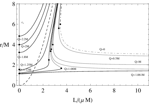
Fig. 21 shows the circular orbits radius as a function of the angular momentum for different black holes and naked singularities. The cases of a Schwarzschild spacetime and the Newtonian limit are also plotted for comparison. Clearly, for large values of $r/M$ all the curves converge to the Newtonian limit.

Finally, the study of the circular orbits stability for neutral test particles in the RN spacetime is summarized in the Fig.22 where the radius of the last stable circular orbits is plotted as function of $Q/M$.

The location and structure of the stability regions for neutral particles around a black hole differ in a very strong way from the case of a naked singularity. Black hole sources are characterized by the existence of only one stability region which can extend from a minimum radius $r_{lsco}\in[4M,6M]$ up to infinity. In the case of a naked singularity there are two possible scenarios. If the mass-to-charge ratio satisfies the condition $Q/M\geq\sqrt{5}/2$, there exist only one stability region which extends from the classical radius $r_{*}=Q^{2}/M$ up to infinity. The second scenario appears in naked singularities with charge-to-mass ratio within the range $1<Q/M<\sqrt{5}/2$. In this case, we have two stability regions separated by either a region of instability or a forbidden region, where no time-like circular orbits are allowed, and a region of instability.

In this work we discussed the motion of neutral test particles along circular orbits in the RN spacetime. We studied separately the case of black holes and naked singularities, emphasizing their differences. Our analysis is based on the study of the behavior of an effective potential that determines the position and stability properties of circular orbits. We also investigated in detail the behavior of the energy and angular momentum of the test particle in all possible configurations of black holes and naked singularities.

We found that at the classical radius $r=r_{*}=Q^{2}/M$ circular orbits exist with “zero” angular momentum. This means that a static observer situated at infinity would interpret this situation as a test particle that remains motionless $(r=Q^{2}/M=$const, $\phi=$const) as time passes. This phenomena can take place only in the case of a naked singularity and is interpreted as a consequence of the “repulsive” force generated by the charge distribution.

Black holes turn out to be characterized by a single zone of stability which extends from a minimum radius $r_{lsco}$ up to infinity. The radius of the last stable circular orbit has its maximum value of $r_{lsco}=6M$ in the Schwarzschild limiting case, and reaches its minimum value of $r_{lsco}=4M$ in the case of an extreme black hole. The situation is completely different in the case of naked singularities. If the mass-to-charge ratio satisfies the condition $Q/M\geq\sqrt{5}/2$, there exist only one stability region which extends from the classical radius $r_{*}=Q^{2}/M$ up to infinity. In this case, the classical radius determines also the radius of the last stable orbit that could be, in principle, as large as allowed by the amount of charge $Q$ that can be associated to a given mass $M$. If the charge-to-mass ratio is within the range $1<Q/M<\sqrt{5}/2$, we found two stability regions that are separated either by a region of instability, in the interval $\sqrt{9/8}<Q/M<\sqrt{5}/2$, or a region of instability and a region forbidden for time-like orbits, in the interval $1<Q/M<\sqrt{9/8}$. This result implies that around a naked singularity with $1<Q/M<\sqrt{5}/2$ the region of stability splits into two non-connected regions in which test particles can remain orbiting forever.

We would like to thank A. Geralico for helpful comments. Two of us (DP and HQ) thank ICRANet support. This work was supported in part by DGAPA-UNAM, grant No. IN106110.

References

• [1] R. Ruffini On the Energetics of Black Holes, Le Astres Occlus, (Le Houche 1972).
• [2] C. W. Misner, K. S. Thorne, and J. A. Wheeler, Gravitation (Freeman, San Francisco, 1973).
• [3] S. Chandrasekhar, The Mathematical Theory of Black Holes (Oxford University Press, New York, 1983).
• [4] J. M. Cohen and R. Gautreau, Phys. Rev. D 19, 2273 (1979).
• [5] P. Pradhan and P. Majumdar, arXiv:1001.0359 [gr-qc].
• [6] V. D. Gladush and M. V. Galadgyi, arXiv:1011.0843 [gr-qc].
• [7] A. N. Aliev, Class. Quant. Grav. 10 (1993) 1741.
• [8] W. B. Bonnor, Phys. Lett. A 83, 414 (1981).
• [9] E. P. T. Liang, Phys. Rev. D 9 (1974) 3257.
• [10] Z. Stuchlik and S. Hledik, Acta Phys. Slov. 52 (2002) 363.
• [11] V. D. Gladush and M. V. Galadgyi, Kinematics and Physics of Celestial Bodies, 2009, Vol. 25, No. 2, pp. 79–88.
• [12] N. Dadhich, J. Math. Phys. 20, 1555 (1979).
• [13] J. Bic̆ák, Z.Stuchlík, and V. Balek, Bull. Astron. Inst. Czech. 40, 65-92 (1989).