跳到论文正文
W Papers独立论文阅读器 arXiv:1012.5390 论文正文 计算阅读时间 · 0%
引用这篇论文根据当前论文元数据生成,正式投稿前建议核对。


License: arXiv.org perpetual non-exclusive license
arXiv:1012.5390v1 [stat.ME] 24 Dec 2010

Forward Smoothing using Sequential Monte Carlo

Pierre Del Moral ††thanks: Centre INRIA Bordeaux et Sud-Ouest & Institut de Mathématiques de Bordeaux , Université de Bordeaux I, 351 cours de la Libération 33405 Talence cedex, France (Pierre.Del-Moral@inria.fr)    Arnaud Doucet ††thanks: The Institute of Statistical Mathematics, 4-6-7 Minami-Azabu, Minato-ku, Tokyo 106-8569, Japan and Department of Statistics & Department of Computer Science, University of British Columbia, 333-6356 Agricultural Road, Vancouver, BC, V6T 1Z2, Canada (Arnaud@stat.ubc.ca)    Sumeetpal S. Singh ††thanks: Department of Engineering, University of Cambridge, Trumpington Street, CB2 1PZ, United Kingdom (sss40@cam.ac.uk)
Technical Report CUED/F-INFENG/TR 638, Cambridge University.
First version September 27th 2009, Second version November 24th 2009, Third version December 12th 2010.
Abstract

Sequential Monte Carlo (SMC) methods are a widely used set of computational tools for inference in non-linear non-Gaussian state-space models. We propose a new SMC algorithm to compute the expectation of additive functionals recursively. Essentially, it is an online or “forward-only” implementation of a forward filtering backward smoothing SMC algorithm proposed in [18]. Compared to the standard path space SMC estimator whose asymptotic variance increases quadratically with time even under favourable mixing assumptions, the asymptotic variance of the proposed SMC estimator only increases linearly with time. This forward smoothing procedure allows us to implement on-line maximum likelihood parameter estimation algorithms which do not suffer from the particle path degeneracy problem.

Some key words: Expectation-Maximization, Forward Filtering Backward Smoothing, Recursive Maximum Likelihood, Sequential Monte Carlo, Smoothing, State-Space Models.

1 Introduction

1.1 State-space models and inference aims

State-space models (SSM) are a very popular class of non-linear and non-Gaussian time series models in statistics, econometrics and information engineering; see for example [7], [19], [20]. An SSM is comprised of a pair of discrete-time stochastic processes, {Xn}n≥0\left\{X_{n}\right\}_{n\mathbb{\geq}0} and {Yn}n≥0\left\{Y_{n}\right\}_{n\geq 0}, where the former is an 𝒳\mathcal{X}-valued unobserved process and the latter is a 𝒴\mathcal{Y}-valued process which is observed. The hidden process {Xn}n≥0\left\{X_{n}\right\}_{n\mathbb{\geq}0} is a Markov process with initial density μθ​(x)\mu_{\theta}\left(x\right) and Markov transition density fθ(x′|x)f_{\theta}\left(\left.x^{\prime}\right|x\right), i.e.

X0∼μθ(⋅) and Xn|(Xn−1=xn−1)∼fθ(⋅|xn−1),n≥1.X_{0}\sim\mu_{\theta}\left(\cdot\right)\text{ and }\left.X_{n}\right|\left(X_{n-1}=x_{n-1}\right)\sim f_{\theta}\left(\left.\cdot\right|x_{n-1}\right),\qquad n\geq 1. (1.1)

It is assumed that the observations {Yn}n≥0\left\{Y_{n}\right\}_{n\geq 0} conditioned upon {Xn}n≥0\left\{X_{n}\right\}_{n\mathbb{\geq}0} are statistically independent and have marginal density gθ(y|x)g_{\theta}\left(\left.y\right|x\right), i.e.

Yn|({Xk}k≥0={xk}k≥0)∼gθ(⋅|xn).\left.Y_{n}\right|\left(\left\{X_{k}\right\}_{k\geq 0}=\left\{x_{k}\right\}_{k\geq 0}\right)\sim g_{\theta}\left(\left.\cdot\right|x_{n}\right). (1.2)

We also assume that μθ​(x)\mu_{\theta}\left(x\right), fθ(x|x′)f_{\theta}\left(\left.x\right|x^{\prime}\right) and gθ(y|x)g_{\theta}\left(\left.y\right|x\right) are densities with respect to (w.r.t.) suitable dominating measures denoted generically as d​xdx and d​ydy. For example, if 𝒳⊆ℝp\mathcal{X}\subseteq\mathbb{R}^{p} and 𝒴⊆ℝq\mathcal{Y}\subseteq\mathbb{R}^{q} then the dominating measures could be the Lebesgue measures. The variable θ\theta in the densities of these random variables are the particular parameters of the model. The set of possible values for θ\theta is denoted Θ\Theta. The model (1.1)-(1.2) is also referred to as a Hidden Markov Model (HMM) in the literature.

For any sequence {zn}n∈ℤ\left\{z_{n}\right\}_{n\in\mathbb{Z}} and integers j≥ij\geq i, let zi:jz_{i:j} denote the set {zi,zi+1,…,zj}\left\{z_{i},z_{i+1},...,z_{j}\right\}. (When j<ij<i this is to be understood as the empty set.) Equations (1.1) and (1.2) define the joint density of (X0:n,Y0:n)\left(X_{0:n},Y_{0:n}\right),

pθ(x0:n,y0:n)=μθ(x0)∏k=1nfθ(xk|xk−1)∏k=0ngθ(yk|xk)p_{\theta}\left(x_{0:n},y_{0:n}\right)=\mu_{\theta}\left(x_{0}\right)\prod\limits_{k=1}^{n}f_{\theta}\left(\left.x_{k}\right|x_{k-1}\right)\prod\limits_{k=0}^{n}g_{\theta}\left(\left.y_{k}\right|x_{k}\right) (1.3)

which yields the marginal likelihood,

pθ(y0:n)=∫pθ(x0:n,y0:n)dx0:n.p_{\theta}\left(y_{0:n}\right)=\int p_{\theta}\left(x_{0:n},y_{0:n}\right)dx_{0:n}. (1.4)

Let sk:𝒳×𝒳→ℝs_{k}:\mathcal{X}\times\mathcal{X}\rightarrow\mathbb{R}, k∈ℕk\in\mathbb{N}, be a sequence of functions and Sn:𝒳n→ℝS_{n}:\mathcal{X}^{n}\rightarrow\mathbb{R}, n∈ℕn\in\mathbb{N}, be the corresponding sequence of additive functionals constructed from sks_{k} as follows11 1 Incorporating dependency of sks_{k} on yky_{k}, i.e. SnS_{n} is the sums of term of the form sk​(xk−1,xk,yk)s_{k}\left(x_{k-1},x_{k},y_{k}\right), is merely a matter of redefining sks_{k} in the computations to follow.

Sn(x0:n)=∑k=1nsk(xk−1,xk).S_{n}\left(x_{0:n}\right)=\sum_{k=1}^{n}s_{k}\left(x_{k-1},x_{k}\right). (1.5)

There are many instances where it is necessary to be able to compute the following expectations recursively in time,

𝒮nθ=𝔼θ[Sn(X0:n)|y0:n].\mathcal{S}_{n}^{\theta}=\mathbb{E}_{\theta}\left[\left.S_{n}\left(X_{0:n}\right)\right|y_{0:n}\right]. (1.6)

The conditioning implies the expectation should be computed w.r.t. the density of X0:nX_{0:n} given Y0:n=y0:nY_{0:n}=y_{0:n}, i.e. pθ(x0:n|y0:n)∝pθ(x0:n,y0:n)p_{\theta}\left(\left.x_{0:n}\right|y_{0:n}\right)\propto p_{\theta}\left(x_{0:n},y_{0:n}\right) and for this reason 𝒮nθ\mathcal{S}_{n}^{\theta} is referred to as a smoothed additive functional.

As the first example of the need to perform such computations, consider the problem of computing the score vector, ∇logpθ(y0:n)\nabla\log p_{\theta}\left(y_{0:n}\right). The score is a vector in ℝd\mathbb{R}^{d} and its ithi^{\text{th}} component is

[∇logpθ(y0:n)]i=∂log pθ(y0:n)∂θi.\left[\nabla\log p_{\theta}\left(y_{0:n}\right)\right]_{i}=\frac{\partial\log\text{ }p_{\theta}\left(y_{0:n}\right)}{\partial\theta^{i}}. (1.7)

Using Fisher’s identity, the problem of computing the score becomes an instance of (1.6), i.e.

∇logpθ(y0:n)\displaystyle\nabla\log p_{\theta}\left(y_{0:n}\right) =∑k=1n𝔼θ[∇logfθ(Xk|Xk−1)|y0:n]+∑k=0n𝔼θ[∇loggθ(yk|Xk)|y0:n]\displaystyle=\sum\limits_{k=1}^{n}\mathbb{E}_{\theta}\left[\left.\nabla\log f_{\theta}\left(\left.X_{k}\right|X_{k-1}\right)\right|y_{0:n}\right]+\sum\limits_{k=0}^{n}\mathbb{E}_{\theta}\left[\left.\nabla\log g_{\theta}\left(\left.y_{k}\right|X_{k}\right)\right|y_{0:n}\right]
+𝔼θ[∇logμθ(X0)|y0:n].\displaystyle+\mathbb{E}_{\theta}\left[\left.\nabla\log\mu_{\theta}\left(X_{0}\right)\right|y_{0:n}\right]. (1.8)

An alternative representation of the score as a smoothed additive functional based on infinitesimal perturbation analysis is given in [12]. The score has applications to Maximum Likelihood (ML) parameter estimation [32], [37].

The second example is ML parameter estimation using the Expectation-Maximization (EM) algorithm. Let y0:ny_{0:n} be a batch of data and the aim is to maximise pθ(y0:n)p_{\theta}\left(y_{0:n}\right) w.r.t. θ\theta. Given a current estimate θ′\theta^{\prime}, a new estimate θ′′\theta^{\prime\prime} is obtained by maximizing the function

Q⁡(θ′,θ)\displaystyle Q\left(\theta^{\prime},\theta\right) =∑k=1n𝔼θ′[logfθ(Xk|Xk−1)|y0:n]+∑k=0n𝔼θ′[loggθ(yk|Xk)|y0:n]\displaystyle=\sum\limits_{k=1}^{n}\mathbb{E}_{\theta^{\prime}}\left[\left.\log f_{\theta}\left(\left.X_{k}\right|X_{k-1}\right)\right|y_{0:n}\right]+\sum\limits_{k=0}^{n}\mathbb{E}_{\theta^{\prime}}\left[\left.\log g_{\theta}\left(\left.y_{k}\right|X_{k}\right)\right|y_{0:n}\right]
+𝔼θ′[logμθ(X0)|y0:n]\displaystyle+\mathbb{E}_{\theta^{\prime}}\left[\left.\log\mu_{\theta}\left(X_{0}\right)\right|y_{0:n}\right]

w.r.t. θ\theta and setting θ′′\theta^{\prime\prime} to the maximising argument. A fundamental property of the EM algorithm is pθ′′(y0:n)≥pθ′(y0:n)p_{\theta^{\prime\prime}}\left(y_{0:n}\right)\geq p_{\theta^{\prime}}\left(y_{0:n}\right). For linear Gaussian models and finite state-space HMM, it is possible to perform the computations in the definition of Q⁡(θ′,θ)Q\left(\theta^{\prime},\theta\right). For general non-linear non-Gaussian state-space models of the form (1.1)-(1.2), we need to rely on numerical approximation schemes.

1.2 Current approaches to smoothing with SMC

SMC methods are a class of algorithms that sequentially approximate the sequence of posterior distributions {pθ(dx0:n|y0:n)}n≥0\left\{p_{\theta}\left(dx_{0:n}|y_{0:n}\right)\right\}_{n\geq 0} using a set of NN weighted random samples called particles. Specifically, the SMC approximation of pθ(dx0:n|y0:n)p_{\theta}\left(dx_{0:n}|y_{0:n}\right), for n≥0n\geq 0, is

p^θ(dx0:n|y0:n):=∑i=1NWn(i)δX0:n(i)(dx0:n), Wn(i)≥0, ∑i=1NWn(i)=1,\widehat{p}_{\theta}\left(dx_{0:n}|y_{0:n}\right):=\sum_{i=1}^{N}W_{n}^{\left(i\right)}\delta_{X_{0:n}^{\left(i\right)}}\left(dx_{0:n}\right),\text{ }W_{n}^{\left(i\right)}\geq 0,\text{\ }\sum_{i=1}^{N}W_{n}^{\left(i\right)}=1, (1.9)

where Wn(i)W_{n}^{\left(i\right)} is the importance weight associated to particle X0:n(i)X_{0:n}^{\left(i\right)} and δX0:n(i)\delta_{X_{0:n}^{\left(i\right)}} is the Dirac measure with an atom at X0:n(i)X_{0:n}^{\left(i\right)}. The particles are propagated forward in time using a combination of importance sampling and resampling steps and there are several variants of both these steps; see [14], [19] for details. SMC methods are parallelisable and flexible, the latter in the sense that SMC approximations of the posterior densities for a variety of SSMs can be constructed quite easily. SMC methods were popularized by the many successful applications to SSM.

1.2.1 Path space and fixed-lag approximations

A SMC approximation of 𝒮nθ\mathcal{S}_{n}^{\theta} may be constructed by replacing pθ(dx0:n|y0:n)p_{\theta}\left(dx_{0:n}|y_{0:n}\right) in Eq. (1.6) with its SMC approximation in Eq. (1.9) - we call this the path space method since the SMC approximation of pθ(dx0:n|y0:n)p_{\theta}\left(dx_{0:n}|y_{0:n}\right), which is a probability distribution on 𝒳n+1\mathcal{X}^{n+1}, is used. Fortunately there is no need to store the entire ancestry of each particle, i.e. {X0:n(i)}1≤i≤N\left\{X_{0:n}^{\left(i\right)}\right\}_{1\leq i\leq N}, which would require a growing memory. Also, this estimate can be computed recursively. However, the reliance on the approximation of the joint distribution pθ(dx0:n|y0:n)p_{\theta}\left(\left.dx_{0:n}\right|y_{0:n}\right) is bad. It is well-known in the SMC literature that the approximation of pθ(dx0:n|y0:n)p_{\theta}\left(\left.dx_{0:n}\right|y_{0:n}\right) becomes progressively impoverished as nn increases because of the successive resampling steps [3], [13], [34]. That is, the number of distinct samples representing pθ(dx0:k|y0:n)p_{\theta}\left(\left.dx_{0:k}\right|y_{0:n}\right) for any fixed k<nk<n diminishes as nn increases – this is known as the particle path degeneracy problem. Hence, whatever being the number of particles, pθ(dx0:k|y0:n)p_{\theta}\left(\left.dx_{0:k}\right|y_{0:n}\right) will eventually be approximated by a single unique particle for all (sufficiently large) nn. This has severe consequences for the SMC estimate 𝒮nθ\mathcal{S}_{n}^{\theta}. In [13], under favourable mixing assumptions, the authors established an upper bound on the 𝕃p\mathbb{L}^{p} error which is proportional to n2/Nn^{2}/\sqrt{N}. Under similar assumptions, it was shown in [37] that the asymptotic variance of this estimate increases at least quadratically with nn. To reduce the variance, alternative methods have been proposed. The technique proposed in [29] relies on the fact that for a SSM with “good” forgetting properties,

pθ(x0:k|y0:n)≈pθ(x0:k|y0:min⁡(k+Δ,n))p_{\theta}\left(\left.x_{0:k}\right|y_{0:n}\right)\approx p_{\theta}\left(\left.x_{0:k}\right|y_{0:\min(k+\Delta,n)}\right) (1.10)

when the horizon Δ\Delta is large enough; that is observations collected after times k+Δk+\Delta bring little additional information about X0:kX_{0:k}. (See [16, Corollary 2.9] for exponential error bounds.) This suggests that a very simple scheme to curb particle degeneracy is to stop updating the SMC estimate beyond time k+Δk+\Delta. This algorithm is trivial to implement but the main practical problem is that of determining an appropriate value for Δ\Delta such that the two densities in Eq. (1.10) are close enough and particle degeneracy is low. These are conflicting requirements. A too small value for the horizon will result in pθ(x0:k|y0:min⁡(k+Δ,n))p_{\theta}\left(\left.x_{0:k}\right|y_{0:\min(k+\Delta,n)}\right) being a poor approximation of pθ(x0:k|y0:n)p_{\theta}\left(\left.x_{0:k}\right|y_{0:n}\right) but the particle degeneracy will be low. On the other hand, a larger horizon improves the approximation in Eq. (1.10) but particle degeneracy will creep in. Automating the selection of Δ\Delta is difficult. Additionally, for any finite Δ\Delta the SMC estimate of 𝒮nθ\mathcal{S}_{n}^{\theta} will suffer from a non vanishing bias even as N→∞N\rightarrow\infty. In [34], for an optimized value of Δ\Delta which is dependent on nn and the typically unknown mixing properties of the model, the SMC estimates of 𝒮nθ\mathcal{S}_{n}^{\theta} based on the approximation in Eq. (1.10) were shown to have an 𝕃p\mathbb{L}^{p} error and bias upper bounded by quantities proportional to n​log⁡n/Nn\log n/\sqrt{N} and n​log⁡n/Nn\log n/N under regularity assumptions.

The computational cost of the SMC approximation of 𝒮nθ\mathcal{S}_{n}^{\theta} computed using either the path space method or the truncated horizon method of [29] is 𝒪⁡(N)\mathcal{O}\left(N\right).

1.2.2 Approximating the smoothing equations

A standard alternative to computing 𝒮nθ\mathcal{S}_{n}^{\theta} is to use SMC approximations of fixed-interval smoothing techniques such as the Forward Filtering Backward Smoothing (FFBS) algorithm [18], [26]. Theoretical results on the SMC approximations of the FFBS algorithm have been recently established in [17]; this includes a central limit theorem and exponential deviation inequalities. In particular, under appropriate mixing assumptions, the authors have obtained time-uniform deviation inequalities for the SMC-FFBS approximations of the marginals {pθ(dxk|y0:n)}0≤k≤n\left\{p_{\theta}\left(dx_{k}|y_{0:n}\right)\right\}_{0\leq k\leq n} [17, Section 5]; see [15] for alternative proofs and complementary results. Let 𝒮^nθ\widehat{\mathcal{S}}_{n}^{\theta} denote the SMC-FFBS estimate of 𝒮nθ\mathcal{S}_{n}^{\theta}. In this work it is established that the asymptotic variance of N​(𝒮^nθ−𝒮nθ)\sqrt{N}\left(\widehat{\mathcal{S}}_{n}^{\theta}-\mathcal{S}_{n}^{\theta}\right) only grows linearly with time nn; a fact which was also alluded to in [15]. The main advantage of the SMC implementation of the FFBS algorithm is that it does not have any tuning parameter other than the number of particles NN. However, the improved theoretical properties comes at a computational price; this algorithm has a computational complexity of 𝒪⁡(N2)\mathcal{O}\left(N^{2}\right) compared to 𝒪⁡(N)\mathcal{O}\left(N\right) for the methods previously discussed. (It is possible to use fast computational methods to reduce the computational cost to 𝒪⁡(N​log⁡N)\mathcal{O}\left(N\log N\right) [30].) Another restriction is that the SMC implementation of the FFBS algorithm does not yield an online algorithm.

1.3 Contributions and organization of the article

The contributions of this article are as follows.

  • •

    We propose an original online implementation of the SMC-FFBS estimate of 𝒮nθ\mathcal{S}_{n}^{\theta}. A particular case of this new algorithm was presented in [36], [37] to compute the score vector (1.7). However, because it was catered to estimating the score, the authors failed to realise its full generality.

  • •

    An upper bound for the non-asymptotic mean square error of the SMC-FFBS estimate 𝒮^nθ\widehat{\mathcal{S}}_{n}^{\theta} of 𝒮nθ\mathcal{S}_{n}^{\theta} is derived under regularity assumptions. It follows from this bound that the asymptotic variance of N​(𝒮^nθ−𝒮nθ)\sqrt{N}\left(\widehat{\mathcal{S}}_{n}^{\theta}-\mathcal{S}_{n}^{\theta}\right) is bounded by a quantity proportional to nn. This complements results recently obtained in [15], [17].

  • •

    We demonstrate how the online implementation of the SMC-FFBS estimate of 𝒮nθ\mathcal{S}_{n}^{\theta} can be applied to the problem of recursively estimating the parameters of a SSM from data. We present original SMC implementations of Recursive Maximum Likelihood (RML) [32], [36], [39] and of the online EM algorithm [25], [22], [23], [33], [8], [28, Section 3.2.]. These SMC implementations do not suffer from the particle path degeneracy problem.

The remainder of this paper is organized as follows. In Section 2 the standard FFBS recursion and its SMC implementation is presented. It is then shown how this recursion and its SMC implementation can be implemented exactly with only a forward pass. A non-asymptotic variance bound is presented in Section 3. Recursive parameter estimation procedures are presented in Section 4 and numerical results are given in Section 5. We conclude in Section 6 and the proof of the main theoretical result is given in the Appendix.

2 Forward smoothing and SMC approximations

We first review the standard FFBS recursion and its SMC approximation [18], [26]. This is then followed by a derivation of a forward-only version of the FFBS recursion and its corresponding SMC implementation. The algorithms presented in this section do not depend on any specific SMC implementation to approximate {pθ(dxn|y0:n)}n≥0\left\{p_{\theta}\left(dx_{n}|y_{0:n}\right)\right\}_{n\geq 0}.

2.1 The forward filtering backward smoothing recursion

Recall the definition of 𝒮nθ\mathcal{S}_{n}^{\theta} in Eq. (1.6). The standard FFBS procedure to compute 𝒮nθ\mathcal{S}_{n}^{\theta} proceeds in two steps. In the first step, which is the forward pass, the filtering densities {pθ(xk|y0:k)}0≤k≤n\{p_{\theta}\left(\left.x_{k}\right|y_{0:k}\right)\}_{0\leq k\leq n} are computed using Bayes’ formula:

pθ(xk+1|y0:k+1)=gθ(yk+1|xk+1)∫fθ(xk+1|xk)pθ(xk|y0:k)dxk∫gθ(yk+1|xk+1′)fθ(xk+1′|xk′)pθ(xk′|y0:k)dxk:k+1′.p_{\theta}\left(\left.x_{k+1}\right|y_{0:k+1}\right)=\frac{g_{\theta}\left(\left.y_{k+1}\right|x_{k+1}\right)\int f_{\theta}\left(\left.x_{k+1}\right|x_{k}\right)p_{\theta}\left(\left.x_{k}\right|y_{0:k}\right)dx_{k}}{\int g_{\theta}\left(\left.y_{k+1}\right|x_{k+1}^{\prime}\right)f_{\theta}\left(\left.x_{k+1}^{\prime}\right|x_{k}^{\prime}\right)p_{\theta}\left(\left.x_{k}^{\prime}\right|y_{0:k}\right)dx_{k:k+1}^{\prime}}.

The second step is the backward pass that computes the following marginal smoothed densities which are needed to evaluate each term in the sum that defines 𝒮nθ\mathcal{S}_{n}^{\theta}:

pθ(xk−1,xk|y0:n)=pθ(xk|y0:n)pθ(xk−1|y0:k−1,xk),1≤k≤n.p_{\theta}\left(\left.x_{k-1},x_{k}\right|y_{0:n}\right)=p_{\theta}\left(\left.x_{k}\right|y_{0:n}\right)p_{\theta}\left(\left.x_{k-1}\right|y_{0:k-1},x_{k}\right),\quad 1\leq k\leq n. (2.1)

where

pθ(xk−1|y0:k−1,xk)=fθ(xk|xk−1)pθ(xk−1|y0:k−1)pθ(xk|y0:k−1).p_{\theta}\left(\left.x_{k-1}\right|y_{0:k-1},x_{k}\right)=\frac{f_{\theta}\left(\left.x_{k}\right|x_{k-1}\right)p_{\theta}\left(\left.x_{k-1}\right|y_{0:k-1}\right)}{p_{\theta}\left(\left.x_{k}\right|y_{0:k-1}\right)}. (2.2)

We compute Eq. (2.1) commencing at k=nk=n and then, decrementing kk each time, until k=1k=1. (Integrating Eq. (2.1) w.r.t. xkx_{k} will yield pθ(xk−1|y0:n)p_{\theta}\left(\left.x_{k-1}\right|y_{0:n}\right) which is needed for the next computation.) To compute 𝒮nθ\mathcal{S}_{n}^{\theta}, nn backward steps must be executed and then nn expectations computed. This must then be repeated at time n+1n+1 to incorporate the effect of the new observation yn+1y_{n+1} on these calculations. Clearly this is not an online procedure for computing {𝒮nθ}n≥1\{\mathcal{S}_{n}^{\theta}\}_{n\geq 1}.

The SMC implementation of the FFBS recursion is straightforward [18]. In the forward pass, we compute and store the SMC approximation p^θ(dxk|y0:k)\widehat{p}_{\theta}\left(\left.dx_{k}\right|y_{0:k}\right) of pθ(dxk|y0:k)p_{\theta}\left(\left.dx_{k}\right|y_{0:k}\right) for k=0,1,…,nk=0,1,\ldots,n. In the backward pass, we simply substitute this SMC approximation in the place of pθ(dxk|y0:k)p_{\theta}\left(\left.dx_{k}\right|y_{0:k}\right) in Eq. (2.1). Let

p^θ(dxk|y0:n)=∑i=1NWk|n(i)δXk(i)(dxk)\widehat{p}_{\theta}\left(\left.dx_{k}\right|y_{0:n}\right)=\sum_{i=1}^{N}W_{k|n}^{\left(i\right)}\delta_{X_{k}^{\left(i\right)}}\left(dx_{k}\right) (2.3)

be the SMC approximation of pθ(dxk|y0:n)p_{\theta}\left(\left.dx_{k}\right|y_{0:n}\right), k≤nk\leq n, initialised at k=nk=n by setting Wn|n(i)=Wn(i)W_{n|n}^{(i)}=W_{n}^{(i)}. By substituting p^θ(dxk−1|y0:k−1)\widehat{p}_{\theta}\left(\left.dx_{k-1}\right|y_{0:k-1}\right) for pθ(xk−1|y0:k−1)p_{\theta}\left(\left.x_{k-1}\right|y_{0:k-1}\right) in Eq. (2.2), we obtain

p^θ(dxk−1|y0:k−1,xk)=∑i=1NWk−1(i)​fθ​(xk|Xk−1(i))​δXk−1(i)​(d​xk−1)∑l=1NWk−1(l)​fθ​(xk|Xk−1(l)).\widehat{p}_{\theta}\left(\left.dx_{k-1}\right|y_{0:k-1},x_{k}\right)=\frac{\sum_{i=1}^{N}W_{k-1}^{(i)}f_{\theta}\left(x_{k}|X_{k-1}^{(i)}\right)\delta_{X_{k-1}^{(i)}}\left(dx_{k-1}\right)}{\sum_{l=1}^{N}W_{k-1}^{(l)}f_{\theta}\left(x_{k}|X_{k-1}^{(l)}\right)}. (2.4)

This approximation is combined with p^θ(dxk|y0:n)\widehat{p}_{\theta}\left(\left.dx_{k}\right|y_{0:n}\right) (see Eq. (2.1)) to obtain

p^θ(dxk−1:k|y0:n)=∑i=1N∑j=1NWk|n(j)Wk−1(i)​fθ​(Xk(j)|Xk−1(i))∑l=1NWk−1(l)​fθ​(Xk(j)|Xk−1(l))δXk−1(i),Xk(j)(dxk−1:k).\widehat{p}_{\theta}(dx_{k-1:k}|y_{0:n})=\sum_{i=1}^{N}\sum_{j=1}^{N}W_{k|n}^{(j)}\frac{W_{k-1}^{(i)}f_{\theta}\left(X_{k}^{(j)}|X_{k-1}^{(i)}\right)}{\sum_{l=1}^{N}W_{k-1}^{(l)}f_{\theta}\left(X_{k}^{(j)}|X_{k-1}^{(l)}\right)}\delta_{X_{k-1}^{(i)},X_{k}^{\left(j\right)}}(dx_{k-1:k}). (2.5)

Marginalising this approximation will give the approximation to p^θ(dxk−1|y0:n)\widehat{p}_{\theta}\left(\left.dx_{k-1}\right|y_{0:n}\right), that is {Wk−1|n(i),Xk−1(i)}1≤i≤N\left\{W_{k-1|n}^{\left(i\right)},X_{k-1}^{\left(i\right)}\right\}_{1\leq i\leq N}, where

Wk−1|n(i)=∑j=1NWk|n(j)​Wk−1(i)​fθ​(Xk(j)|Xk−1(i))∑l=1NWk−1(l)​fθ​(Xk(j)|Xk−1(l)).W_{k-1|n}^{(i)}=\sum_{j=1}^{N}W_{k|n}^{(j)}\frac{W_{k-1}^{(i)}f_{\theta}\left(X_{k}^{(j)}|X_{k-1}^{(i)}\right)}{\sum_{l=1}^{N}W_{k-1}^{(l)}f_{\theta}\left(X_{k}^{(j)}|X_{k-1}^{(l)}\right)}. (2.6)

The SMC estimate 𝒮^nθ\widehat{\mathcal{S}}_{n}^{\theta} of 𝒮nθ\mathcal{S}_{n}^{\theta} is then given by

𝒮^nθ=∑k=1n∫sk(xk−1,xk)p^θ(dxk−1:k|y0:n).\widehat{\mathcal{S}}_{n}^{\theta}=\sum\limits_{k=1}^{n}\int s_{k}\left(x_{k-1},x_{k}\right)\widehat{p}_{\theta}(dx_{k-1:k}|y_{0:n}). (2.7)

The backward recursion for the weights, given in Eq. (2.6), makes this an off-line algorithm for computing 𝒮^nθ\widehat{\mathcal{S}}_{n}^{\theta}.

2.2 A forward only version of the forward filtering backward smoothing recursion

To circumvent the need for the backward pass in the computation of 𝒮nθ\mathcal{S}_{n}^{\theta}, the following auxiliary function (on 𝒳\mathcal{X}) is introduced,

Tnθ(xn):=∫Sn(x0:n) pθ(x0:n−1|y0:n−1,xn)dx0:n−1.T_{n}^{\theta}\left(x_{n}\right):=\int S_{n}\left(x_{0:n}\right)\text{ }p_{\theta}\left(\left.x_{0:n-1}\right|y_{0:n-1},x_{n}\right)dx_{0:n-1}. (2.8)

It is apparent that

𝒮nθ=∫Tnθ(xn)pθ(xn|y0:n)dxn.\mathcal{S}_{n}^{\theta}=\int T_{n}^{\theta}\left(x_{n}\right)p_{\theta}\left(\left.x_{n}\right|y_{0:n}\right)dx_{n}. (2.9)

The following proposition establishes a forward recursion to compute {Tnθ}n≥0\{T_{n}^{\theta}\}_{n\geq 0}, which is henceforth referred to as the forward smoothing recursion. For sake of completeness, the proof of this proposition is given.

Proposition 2.1

For n≥1n\geq 1, we have

Tnθ(xn)=∫[Tn−1θ(xn−1)+sn(xn−1,xn)]pθ(xn−1|y0:n−1,xn)dxn−1,T_{n}^{\theta}\left(x_{n}\right)=\int\left[T_{n-1}^{\theta}\left(x_{n-1}\right)+s_{n}\left(x_{n-1},x_{n}\right)\right]p_{\theta}\left(\left.x_{n-1}\right|y_{0:n-1},x_{n}\right)dx_{n-1}, (2.10)

where T0θ​(x0):=0T_{0}^{\theta}\left(x_{0}\right):=0.

Proof. The proof is straightforward

Tnθ​(xn)\displaystyle T_{n}^{\theta}\left(x_{n}\right) :=∫[Sn−1(x0:n−1)+sn(xn−1,xn)] pθ(x0:n−1|y0:n−1,xn)dx0:n−1\displaystyle:=\int\left[S_{n-1}\left(x_{0:n-1}\right)+s_{n}\left(x_{n-1},x_{n}\right)\right]\text{ }p_{\theta}\left(\left.x_{0:n-1}\right|y_{0:n-1},x_{n}\right)dx_{0:n-1}
=∫[∫Sn−1(x0:n−1)pθ(x0:n−2|y0:n−2,xn−1)dx0:n−2]pθ(xn−1|y0:n−1,xn)dxn−1\displaystyle=\int\left[\int S_{n-1}\left(x_{0:n-1}\right)p_{\theta}\left(\left.x_{0:n-2}\right|y_{0:n-2},x_{n-1}\right)dx_{0:n-2}\right]p_{\theta}\left(\left.x_{n-1}\right|y_{0:n-1},x_{n}\right)dx_{n-1}
+∫sn(xn−1,xn) pθ(xn−1|y0:n−1,xn)dxn−1.\displaystyle+\int s_{n}\left(x_{n-1},x_{n}\right)\text{ }p_{\theta}\left(\left.x_{n-1}\right|y_{0:n-1},x_{n}\right)dx_{n-1}.

The integrand in the first equality is Sn(x0:n)S_{n}\left(x_{0:n}\right) while the integrand in the first integral of the second equality is Tn−1θ​(xn−1)T_{n-1}^{\theta}\left(x_{n-1}\right). ■\blacksquare

This recursion is not new and is actually a special instance of dynamic programming for Markov processes; see for example [5]. For a fully observed Markov process with transition density {fθ(xk|xk−1)}k≥1\left\{f_{\theta}\left(\left.x_{k}\right|x_{k-1}\right)\right\}_{k\geq 1}, the dynamic programming recursion to compute the expectation of Sn(x0:n)S_{n}\left(x_{0:n}\right) with respect to the law of the Markov process is usually implemented using a backward recursion going from time nn to time 00. In the partially observed scenario considered here, {Xk}0≤k≤n\left\{X_{k}\right\}_{0\leq k\leq n} conditional on y0:ny_{0:n} is a “backward” Markov process with non-homogeneous transition densities {pθ(xk−1|y0:k−1,xk)}1≤k≤n\left\{p_{\theta}\left(\left.x_{k-1}\right|y_{0:k-1},x_{k}\right)\right\}_{1\leq k\leq n}. Thus (2.10) is the corresponding dynamic programming recursion to compute 𝒮nθ\mathcal{S}_{n}^{\theta} with respect to pθ(x0:n|y0:n)p_{\theta}\left(\left.x_{0:n}\right|y_{0:n}\right) for this backward Markov chain. This recursion is the foundation of the online EM algorithm and is described at length in [21] (pioneered in [40]) where the density pθ(xn−1|y0:n−1,xn)p_{\theta}\left(\left.x_{n-1}\right|y_{0:n-1},x_{n}\right) appearing in Tnθ​(xn)T_{n}^{\theta}\left(x_{n}\right) is usually written as

pθ(xn−1|y0:n−1,xn)=fθ(xn|xn−1)pθ(xn−1,y0:n−1)∫fθ(xn|xn−1)pθ(xn−1,y0:n−1)dxn−1p_{\theta}\left(\left.x_{n-1}\right|y_{0:n-1},x_{n}\right)=\frac{f_{\theta}\left(x_{n}|x_{n-1}\right)p_{\theta}\left(x_{n-1},y_{0:n-1}\right)}{\int f_{\theta}\left(x_{n}|x_{n-1}\right)p_{\theta}\left(x_{n-1},y_{0:n-1}\right)dx_{n-1}}

or as in Eq. (2.2) in [8], [9], [15]. The forward smoothing recursion has been rediscovered independently several times; see [27], [33] for example.

A simple SMC scheme to approximate 𝒮nθ\mathcal{S}_{n}^{\theta} can be devised by exploiting equations (2.9) and (2.10). This is summarised as Algorithm SMC-FS below.


Algorithm SMC-FS: Forward-only SMC computation of the FFBS estimate

∙\bullet Assume at time n−1n-1 that SMC approximations {Wn−1(i),Xn−1(i)}1≤i≤N\left\{W_{n-1}^{\left(i\right)},X_{n-1}^{\left(i\right)}\right\}_{1\leq i\leq N} of pθ(dxn−1|y0:n−1)p_{\theta}\left(\left.dx_{n-1}\right|y_{0:n-1}\right) and {T^n−1θ​(Xn−1(i))}1≤i≤N\left\{\widehat{T}_{n-1}^{\theta}\left(X_{n-1}^{\left(i\right)}\right)\right\}_{1\leq i\leq N} of {Tn−1θ​(Xn−1(i))}1≤i≤N\left\{T_{n-1}^{\theta}\left(X_{n-1}^{\left(i\right)}\right)\right\}_{1\leq i\leq N} are available.

∙\bullet At time nn, compute the SMC approximation {Wn(i),Xn(i)}1≤i≤N\left\{W_{n}^{\left(i\right)},X_{n}^{\left(i\right)}\right\}_{1\leq i\leq N} of pθ(dxn|y0:n)p_{\theta}\left(\left.dx_{n}\right|y_{0:n}\right) and set

T^nθ​(Xn(i))\displaystyle\widehat{T}_{n}^{\theta}\left(X_{n}^{\left(i\right)}\right) =∑j=1NWn−1(j)​fθ​(Xn(i)|Xn−1(j))​[T^n−1θ​(Xn−1(j))+sn​(Xn−1(j),Xn(i))]∑j=1NWn−1(j)​fθ​(Xn(i)|Xn−1(j)),1≤i≤N,\displaystyle=\frac{\sum_{j=1}^{N}W_{n-1}^{\left(j\right)}f_{\theta}\left(X_{n}^{(i)}|X_{n-1}^{(j)}\right)\left[\widehat{T}_{n-1}^{\theta}\left(X_{n-1}^{\left(j\right)}\right)+s_{n}\left(X_{n-1}^{\left(j\right)},X_{n}^{\left(i\right)}\right)\right]}{\sum_{j=1}^{N}W_{n-1}^{\left(j\right)}f_{\theta}\left(X_{n}^{(i)}|X_{n-1}^{(j)}\right)},\quad 1\leq i\leq N, (2.11)
𝒮^nθ\displaystyle\widehat{\mathcal{S}}_{n}^{\theta} =∑i=1NWn(i) T^nθ(Xn(i)).\displaystyle=\sum_{i=1}^{N}W_{n}^{\left(i\right)}\text{ }\widehat{T}_{n}^{\theta}\left(X_{n}^{\left(i\right)}\right). (2.12)


This algorithm is initialized by setting T^0θ​(X0(i))=0\widehat{T}_{0}^{\theta}\left(X_{0}^{\left(i\right)}\right)=0 for 1≤i≤N.1\leq i\leq N. It has a computational complexity of 𝒪⁡(N2)\mathcal{O}\left(N^{2}\right) which can be reduced by using fast computational methods [30].

The rationale for this algorithm is as follows. By using p^θ(dxn−1|y0:n−1,xn)\widehat{p}_{\theta}\left(\left.dx_{n-1}\right|y_{0:n-1},x_{n}\right) defined in Eq. (2.4) in place of pθ(dxn−1|y0:n−1,xn)p_{\theta}\left(\left.dx_{n-1}\right|y_{0:n-1},x_{n}\right) in Eq. (2.10), we obtain an approximation T^nθ​(xn)\widehat{T}_{n}^{\theta}\left(x_{n}\right) of Tnθ​(xn)T_{n}^{\theta}\left(x_{n}\right) which is computed at the particle locations {Xn(i)}1≤i≤N\left\{X_{n}^{\left(i\right)}\right\}_{1\leq i\leq N}. The approximation of 𝒮nθ\mathcal{S}_{n}^{\theta} in Eq. (2.12) now follows from Eq. (2.9) by using p^θ(dxn|y0:n)\widehat{p}_{\theta}\left(\left.dx_{n}\right|y_{0:n}\right) in place of pθ(dxn|y0:n)p_{\theta}\left(\left.dx_{n}\right|y_{0:n}\right).

It is valid to use the same notation for the estimates in Eq. (2.7) and in Eq. (2.12) as they are indeed the same. The verification of this assertion may be accomplished by unfolding the recursion in Eq. (2.11).

3 Theoretical results

In this section, we present a bound on the non-asymptotic mean square error of the estimate 𝒮^nθ\widehat{\mathcal{S}}_{n}^{\theta} of 𝒮nθ\mathcal{S}_{n}^{\theta}. For sake of simplicity, the result is established for additive functionals of the type

Sn(x0:n)=∑k=0nsk(xk)S_{n}\left(x_{0:n}\right)=\sum_{k=0}^{n}s_{k}\left(x_{k}\right) (3.1)

where sk:𝒳→ℝs_{k}:\mathcal{X}\rightarrow\mathbb{R}, and when Algorithm SMC-FS is implemented using the bootstrap particle filter; see [7], [19] for a definition of this “vanilla” particle filter. The result can be generalised to accommodate an auxiliary implementation of the particle filter [6], [17], [35]. Likewise, the conclusion is also valid for additive functionals of the type in (1.5); the proof uses similar arguments but is more complicated.

The following regularity condition will be assumed.

(A) There exist constants 0<ρ,δ<∞0<\rho,\delta<\infty such that for all x,x′∈𝒳x,x^{\prime}\in\mathcal{X}, y∈𝒴y\in\mathcal{Y} and θ∈Θ\theta\in\Theta,

ρ−1≤fθ​(x′|x)≤ρ,δ−1≤gθ​(y|x)≤δ.\rho^{-1}\leq f_{\theta}\left(x^{\prime}|x\right)\leq\rho,\quad\delta^{-1}\leq g_{\theta}\left(y|x\right)\leq\delta.

Admittedly, this assumption is restrictive and typically holds when 𝒳\mathcal{X} and 𝒴\mathcal{Y} are finite or are compact spaces. In general, quantifying the errors of SMC approximations under weaker assumptions is possible [17]. (More precise but complicated error bounds for the particle estimate of 𝒮nθ\mathcal{S}_{n}^{\theta} are also presented in [15] under weaker assumptions.) However, when (A) holds, the bounds can be greatly simplified to the extent that they can usually be expressed as linear or quadratic functions of the time horizon nn. These simple rates of growth are meaningful as they have also been observed in numerical studies even in scenarios where Assumption A is not satisfied [37].

For a function s:𝒳→ℝs:\mathcal{X}\rightarrow\mathbb{R}, let ‖s‖=supx∈𝒳|s⁡(x)|\left\|s\right\|=\sup_{x\in\mathcal{X}}|s(x)|. The oscillation of ss, denoted osc​(s)\mbox{osc}(s), is defined to be sup{|s⁡(x)−s⁡(y)|;x,y∈𝒳}\sup{\{|s(x)-s(y)|\;;\;x,y\in\mathcal{X}\}}. The main result in this section is the following non-asymptotic bound for the mean square error of the estimate 𝒮^nθ\widehat{\mathcal{S}}_{n}^{\theta} of 𝒮nθ\mathcal{S}_{n}^{\theta} given in Eq. (2.12).

Theorem 3.1

Assume (A). Consider the additive functional SnS_{n} in (3.1) with ‖sk‖<∞\left\|s_{k}\right\|<\infty and osc​(sk)≤1\mbox{osc}(s_{k})\leq 1 for 0≤k≤n0\leq k\leq n. Then, for any n≥0n\geq 0 and θ∈Θ\theta\in\Theta,

𝔼⁡(|𝒮^nθ−𝒮nθ|2)≤a​(n+1)N​(1+n+1N)2\mathbb{E}\left(\left|\widehat{\mathcal{S}}_{n}^{\theta}-\mathcal{S}_{n}^{\theta}\right|^{2}\right)\leq a~\frac{(n+1)}{N}\left(1+\sqrt{\frac{n+1}{N}}\right)^{2} (3.2)

where aa is a finite constant that is independent of time nn, θ\theta and the particular choice of functions {sk}0≤k≤n\{s_{k}\}_{0\leq k\leq n}.

The proof is given in the Appendix. It follows that the asymptotic variance ofN​(𝒮^nθ−𝒮nθ)\sqrt{N}\left(\widehat{\mathcal{S}}_{n}^{\theta}-\mathcal{S}_{n}^{\theta}\right), i.e. as the number of particles NN goes to infinity, is upper bounded by a quantity proportional to (n+1)(n+1) as the bias of the estimate is 𝒪⁡(1/N)\mathcal{O}(1/N) [15, Corollary 5.3].

Let ℛ^nθ\widehat{\mathcal{R}}_{n}^{\theta} denote the SMC estimate of 𝒮nθ\mathcal{S}_{n}^{\theta} obtained with the standard path space method. This estimate can have a much larger asymptotic variance as is illustrated with the following very simple model. Let fθ​(x′|x)=μθ​(x′)f_{\theta}\left(x^{\prime}|x\right)=\mu_{\theta}\left(x^{\prime}\right), i.e. {Xn}n≥0\{X_{n}\}_{n\geq 0} is an i.i.d. sequence, and let yk=yy_{k}=y and sk=ss_{k}=s for all k≥1k\geq 1 where ss is some real valued function on 𝒳\mathcal{X}, and s0=0s_{0}=0. It can be easily established that the formula for the asymptotic variance of N​(ℛ^nθ−𝒮nθ)\sqrt{N}\left(\widehat{\mathcal{R}}_{n}^{\theta}-\mathcal{S}_{n}^{\theta}\right) given in [11], [14, eqn. (9.13), page 304 ] simplifies to

n∫[πθ(x|y)s~θ(x)]2μθ​(x)dx+n⁡(n−1)2∫πθ(x|y)2μθ​(x)dx ∫s~θ(x)2πθ(x|y)dxn\int\frac{\left[\pi_{\theta}\left(\left.x\right|y\right)\widetilde{s}_{\theta}\left(x\right)\right]^{2}}{\mu_{\theta}\left(x\right)}dx+\frac{n\left(n-1\right)}{2}\int\frac{\pi_{\theta}\left(\left.x\right|y\right)^{2}}{\mu_{\theta}\left(x\right)}dx\text{ }\int\widetilde{s}_{\theta}\left(x\right)^{2}\pi_{\theta}\left(\left.x\right|y\right)dx (3.3)

where

πθ(x|y)\displaystyle\pi_{\theta}\left(\left.x\right|y\right) =μθ(x)gθ(y|x)∫μθ(x′)gθ(y|x′)dx′,\displaystyle=\frac{\mu_{\theta}\left(x\right)g_{\theta}\left(\left.y\right|x\right)}{\int\mu_{\theta}\left(x^{\prime}\right)g_{\theta}\left(\left.y\right|x^{\prime}\right)dx^{\prime}},
s~θ​(x)\displaystyle\widetilde{s}_{\theta}\left(x\right) =s(x)−∫s(x)πθ(x|y)dx.\displaystyle=s\left(x\right)-\int s\left(x\right)\pi_{\theta}\left(\left.x\right|y\right)dx.

Thus the asymptotic variance increases quadratically with time nn. Note though that the asymptotic variance of N​(n−1​ℛ^nθ−n−1​𝒮nθ)\sqrt{N}\left(n^{-1}\widehat{\mathcal{R}}_{n}^{\theta}-n^{-1}\mathcal{S}_{n}^{\theta}\right) converges as nn tends to infinity to a positive constant. Thus path space method can provide stable estimates of 𝔼θ[n−1Sn(X0:n)|y0:n]\mathbb{E}_{\theta}\left[\left.n^{-1}S_{n}\left(X_{0:n}\right)\right|y_{0:n}\right], i.e. when the additive functionals are time-averaged. Let

Sγ,n(x0:n)=γns(xn)+∑k=1n−1s(xk)γk∏i=k+1n(1−γi)S_{\gamma,n}\left(x_{0:n}\right)=\gamma_{n}s(x_{n})+\sum_{k=1}^{n-1}s\left(x_{k}\right)\gamma_{k}\prod\limits_{i=k+1}^{n}(1-\gamma_{i})

where {γn}n≥1\left\{\gamma_{n}\right\}_{n\geq 1} is a positive non-increasing sequence that satisfies the following constraints: ∑nγn=∞\sum_{n}\gamma_{n}=\infty and ∑nγn2<∞\sum_{n}\gamma_{n}^{2}<\infty. When γn=n−1\gamma_{n}=n^{-1} then Sγ,n(x0:n)=n−1Sn(x0:n)S_{\gamma,n}\left(x_{0:n}\right)=n^{-1}S_{n}\left(x_{0:n}\right). One important choice for recursive parameter estimation (see Section 4) is

γn=n−α,0.5<α≤1.\gamma_{n}=n^{-\alpha},\quad 0.5<\alpha\leq 1. (3.4)

It is also of interest to quantify the stability of the path space method when applied to estimate 𝒮nθ=𝔼θ[Sγ,n(X0:n)|y0:n]\mathcal{S}_{n}^{\theta}=\mathbb{E}_{\theta}\left[\left.S_{\gamma,n}\left(X_{0:n}\right)\right|y_{0:n}\right] in this more general time-averaging setting. Once again let ℛ^nθ\widehat{\mathcal{R}}_{n}^{\theta} denote the SMC estimate of 𝔼θ[Sγ,n(X0:n)|y0:n]\mathbb{E}_{\theta}\left[\left.S_{\gamma,n}\left(X_{0:n}\right)\right|y_{0:n}\right] obtained with the standard path space method. Using the formula for the asymptotic variance of N​(ℛ^nθ−𝒮nθ)\sqrt{N}\left(\widehat{\mathcal{R}}_{n}^{\theta}-\mathcal{S}_{n}^{\theta}\right) given in [11], [14, eqn. (9.13), page 304 ] it can be verified that this asymptotic variance is

∫[πθ(x|y)s~θ(x)]2μθ​(x)​𝑑x​∑k=1nγk2​∏i=k+1n(1−γi)2\displaystyle\int\frac{\left[\pi_{\theta}\left(\left.x\right|y\right)\widetilde{s}_{\theta}\left(x\right)\right]^{2}}{\mu_{\theta}\left(x\right)}dx\sum\limits_{k=1}^{n}\gamma_{k}^{2}\prod\limits_{i=k+1}^{n}(1-\gamma_{i})^{2}
+∫πθ(x|y)2μθ​(x)dx ∫s~θ(x)2πθ(x|y)dx∑k=2n∑i=1k−1γi2(1−γi+1)2⋯(1−γn)2\displaystyle+\int\frac{\pi_{\theta}\left(\left.x\right|y\right)^{2}}{\mu_{\theta}\left(x\right)}dx\text{ }\int\widetilde{s}_{\theta}\left(x\right)^{2}\pi_{\theta}\left(\left.x\right|y\right)dx\sum\limits_{k=2}^{n}\sum\limits_{i=1}^{k-1}\gamma_{i}^{2}(1-\gamma_{i+1})^{2}\cdots(1-\gamma_{n})^{2}

It follows from Lemma A.4 in Appendix that any accumulation point of this sequence (in nn) has to be positive. In contrast, the asymptotic variance of N​(𝒮^nθ−𝒮nθ)\sqrt{N}(\widehat{\mathcal{S}}_{n}^{\theta}-\mathcal{S}_{n}^{\theta}), i.e. when 𝔼θ[Sγ,n(X0:n)|y0:n]\mathbb{E}_{\theta}\left[\left.S_{\gamma,n}\left(X_{0:n}\right)\right|y_{0:n}\right] is computed using Algorithm SMC-FS, will converge to zero as nn tends to infinity.

4 Application to SMC parameter estimation

An important application of the forward smoothing recursion is to parameter estimation for non-linear non-Gaussian SSMs. We will assume that observations are generated from an unknown ‘true’ model with parameter value θ∗∈Θ\theta^{\ast}\in\Theta, i.e. Xn|(Xn−1=xn−1)∼fθ∗(⋅|xn−1)X_{n}|(X_{n-1}=x_{n-1})\sim f_{\theta^{\ast}}(\cdot|x_{n-1}) and Yn|(Xn=xn)∼gθ∗(⋅|xn)Y_{n}|(X_{n}=x_{n})\sim g_{\theta^{\ast}}(\cdot|x_{n}). The static parameter estimation problem has generated a lot of interest over the past decade and many SMC techniques have been proposed to solve it; see [28] for a recent review.

4.1 Brief literature review

In a Bayesian approach to the problem, a prior distribution is assigned to θ\theta and the sequence of posterior densities {p(θ,x0:n|y0:n)}n≥0\{p\left(\theta,x_{0:n}|y_{0:n}\right)\}_{n\geq 0} is estimated recursively using SMC algorithms combined with Markov chain Monte Carlo (MCMC) steps [1], [24], [38]. Unfortunately these methods suffer from the particle path degeneracy problem and will result in unreliable estimates of the model parameters; see [3], [34] for a discussion of this issue. Given a fixed observation record y0:ny_{0:n}, an alternative offline MCMC approach to estimate p(θ,x0:n|y0:n)p\left(\theta,x_{0:n}|y_{0:n}\right) has been recently proposed which relies on proposals built using the SMC approximation of pθ(x0:n|y0:n)p_{\theta}\left(\left.x_{0:n}\right|y_{0:n}\right) [2].

In a ML approach, the estimate of θ∗\theta^{\ast} is the maximising argument of the likelihood of the observed data. The ML estimate can be calculated using a gradient ascent algorithm either offline for a fixed batch of data or online [32]; see Section 4.2. Likewise, the EM algorithm can also be implemented offline or online. The online EM algorithm, assuming all calculations can be performed exactly, is presented in [25], [22], [23], [33] and [9]. For a general SSM for which the quantities required by the online EM cannot be calculated exactly, an SMC implementation is possible [8], [28, Section 3.2.]; see Section 4.3.

4.2 Gradient ascent algorithms

To maximise the likelihood pθ(y0:n)p_{\theta}(y_{0:n}) w.r.t. θ\theta, we can use a simple gradient algorithm. Let {θi}i∈ℕ\{\theta_{i}\}_{i\in\mathbb{N}} be the sequence of parameter estimates of the gradient algorithm. We update the parameter at iteration i+1i+1 using

θi+1=θi+γi+1∇logpθ(y0:n)|θ=θi\theta_{i+1}=\theta_{i}+\gamma_{i+1}\left.\nabla\log p_{\theta}\left(y_{0:n}\right)\right|_{\theta=\theta_{i}}

where ∇logpθ(y0:n)|θ=θi\left.\nabla\log p_{\theta}\left(y_{0:n}\right)\right|_{\theta=\theta_{i}} is the score vector computed at θ=θi\theta=\theta_{i} and {γi}i≥1\left\{\gamma_{i}\right\}_{i\geq 1} is a sequence of positive non-increasing step-sizes defined in (3.4). For a general SSM, we need to approximate ∇logpθ(y0:n)|θ=θi\left.\nabla\log p_{\theta}\left(y_{0:n}\right)\right|_{\theta=\theta_{i}}. As mentioned in the introduction, the score vector admits several smoothed additive functional representations; see Eq. (1.7) and [12]. Using Eq. (1.7), it is possible to approximate the score with Algorithm SMC-FS.

In the online implementation, the parameter estimate at time n+1n+1 is updated according to [4], [32]

θn+1=θn+γn+1∇logpθ0:n(yn|y0:n−1)\theta_{n+1}=\theta_{n}+\gamma_{n+1}\nabla\log p_{\theta_{0:n}}(y_{n}|y_{0:n-1}) (4.1)

Upon receiving yny_{n}, θn\theta_{n} is updated in the direction of ascent of the predictive density of this new observation. A necessary requirement for an online implementation is that the previous values of the model parameter estimates (other than θn\theta_{n}) are also used in the evaluation of ∇θlogpθ(yn|y0:n−1)\nabla_{\theta}\log p_{\theta}(y_{n}|y_{0:n-1}) at θ=θn\theta=\theta_{n}. This is indicated in the notation ∇logpθ0:n(yn|y0:n−1)\nabla\log p_{\theta_{0:n}}(y_{n}|y_{0:n-1}). (Not doing so would require browsing through the entire history of observations.) This approach was suggested by [32] for the finite state-space case and is named RML. The asymptotic properties of this algorithm (i.e. the behavior of θn\theta_{n} in the limit as nn goes to infinity) have been studied in the case of an i.i.d. hidden process by [39] and for an HMM with a finite state-space by [32]. Under suitable regularity assumptions, convergence to θ∗\theta^{\ast} and a central limit theorem for the estimation error has been established.

For a general SSM, we can compute a SMC estimate of ∇logpθ0:n(yn|y0:n−1)\nabla\log p_{\theta_{0:n}}(y_{n}|y_{0:n-1}) using Algorithm SMC-FS upon noting that ∇logpθ0:n(yn|y0:n−1)\nabla\log p_{\theta_{0:n}}(y_{n}|y_{0:n-1}) is equal to

∇logpθ0:n(y0:n)−∇logpθ0:n−1(y0:n−1).\nabla\log p_{\theta_{0:n}}(y_{0:n})-\nabla\log p_{\theta_{0:n-1}}(y_{0:n-1}).

In particular, at time nn, a particle approximation {Wn(i),Xn(i)}1≤i≤N\left\{W_{n}^{\left(i\right)},X_{n}^{\left(i\right)}\right\}_{1\leq i\leq N} of pθ0:n(dxn|y0:n)p_{\theta_{0:n}}\left(\left.dx_{n}\right|y_{0:n}\right) is computed using the particle approximation at time n−1n-1 and parameter value θ=θn\theta=\theta_{n}. Similarly, the computation of Eq. (2.11) is performed using θ=θn\theta=\theta_{n} and with

sn(xn−1,xn)=∇logfθ(xn|xn−1)|θ=θn+∇loggθ(yn|xn)|θ=θn.s_{n}(x_{n-1},x_{n})=\left.\nabla\log f_{\theta}\left(\left.x_{n}\right|x_{n-1}\right)\right|_{\theta=\theta_{n}}+\left.\nabla\log g_{\theta}\left(\left.y_{n}\right|x_{n}\right)\right|_{\theta=\theta_{n}}.

The estimate of ∇logpθ0:n(yn|y0:n−1)\nabla\log p_{\theta_{0:n}}(y_{n}|y_{0:n-1}) is now the difference of the estimate in Eq. (2.12) with the same estimate computed at time n−1n-1.

Under the regularity assumptions given in Section 3, it follows from the results in the Appendix that the asymptotic variance (i.e. as N→∞N\rightarrow\infty) of the SMC estimate of ∇logpθ0:n(yn|y0:n−1)\nabla\log p_{\theta_{0:n}}(y_{n}|y_{0:n-1}) computed using Algorithm SMC-FS is uniformly (in time) bounded. On the contrary, the standard path-based SMC estimate of ∇logpθ0:n(yn|y0:n−1)\nabla\log p_{\theta_{0:n}}(y_{n}|y_{0:n-1}) has an asymptotic variance that increases linearly with nn.

4.3 EM algorithms

Gradient ascent algorithms are more generally applicable than the EM algorithm. However, their main drawback in practice is that it is difficult to properly scale the components of the computed gradient vector. For this reason the EM algorithm is usually favoured by practitioners whenever it is applicable.

Let {θi}i∈ℕ\{\theta_{i}\}_{i\in\mathbb{N}} be the sequence of parameter estimates of the EM algorithm. In the offline approach, at iteration i+1i+1, the function

Q(θi,θ)=∫logpθ(x0:n,y0:n) pθi(x0:n|y0:n)dx0:nQ(\theta_{i},\theta)=\int\log p_{\theta}(x_{0:n},y_{0:n})\text{ }p_{\theta_{i}}(x_{0:n}|y_{0:n})dx_{0:n}

is computed and then maximized. The maximizing argument is the new estimate θi+1\theta_{i+1}. If pθ(x0:n,y0:n)p_{\theta}(x_{0:n},y_{0:n}) belongs to the exponential family, then the maximization step is usually straightforward. We now give an example of this.

Let sl:𝒳×𝒳×𝒴→ℝs^{l}:\mathcal{X\times X\times Y}\rightarrow\mathbb{R}, l=1,…,ml=1,\ldots,m, be a collection of functions with corresponding additive functionals

Sl,n(x0:n,y0:n)=∑k=1nsl(xk−1,xk,yk),1≤l≤m,S_{l,n}(x_{0:n},y_{0:n})=\sum_{k=1}^{n}s^{l}\left(x_{k-1},x_{k},y_{k}\right),\qquad 1\leq l\leq m,

and let

𝒮l,nθ=∫Sl,n(x0:n,y0:n)pθ(x0:n|y0:n)dx0:n.\mathcal{S}_{l,n}^{\theta}=\int S_{l,n}(x_{0:n},y_{0:n})p_{\theta}(x_{0:n}|y_{0:n})dx_{0:n}.

The collection {𝒮l,nθ}1≤l≤m\{\mathcal{S}_{l,n}^{\theta}\}_{1\leq l\leq m} is also referred to as the summary statistics in the literature. Typically, the maximising argument of Q⁡(θi,θ)Q(\theta_{i},\theta) can be characterised explicitly through a suitable function Λ:ℝm→Θ\Lambda:\mathbb{R}^{m}\rightarrow\Theta, i.e.

θi+1=Λ⁡(n−1​𝒮nθi)\theta_{i+1}=\Lambda\left(n^{-1}\mathcal{S}_{n}^{\theta_{i}}\right) (4.2)

where [𝒮nθ]l=𝒮l,nθ[\mathcal{S}_{n}^{\theta}]_{l}=\mathcal{S}_{l,n}^{\theta}. As an example of this, consider the following stochastic volatility model [35].

Example 4.1

The stochastic volatility model is a SSM defined by the following equations:

X0\displaystyle X_{0} ∼𝒩(0,σ21−ϕ2), Xn+1=ϕXn+σVn+1,\displaystyle\sim\mathcal{N}\left(0,\frac{\sigma^{2}}{1-\phi^{2}}\right),\text{ }X_{n+1}=\phi X_{n}+\sigma V_{n+1},
Yn\displaystyle Y_{n} =β​exp⁡(Xn/2)​Wn,\displaystyle=\beta\exp\left(X_{n}/2\right)W_{n},

where {Vn}n∈ℕ\{V_{n}\}_{n\in\mathbb{N}} and {Wn}n≥0\{W_{n}\}_{n\geq 0} are independent and identically distributed standard normal noise sequences, which are also independent of each other and of the initial state X0X_{0}. The model parameters θ≜(ϕ,σ2,β2)∈ℝ×(0,∞)×(0,∞)\theta\triangleq\left(\phi,\sigma^{2},\beta^{2}\right)\in\mathbb{R\times(}0,\infty\mathbb{)}\times\mathbb{(}0,\infty\mathbb{)} are to be estimated. To apply the EM algorithm to this model, let

s1​(xn−1,xn,yn)\displaystyle s^{1}\left(x_{n-1},x_{n},y_{n}\right) =xn−1xn, s2(xn−1,xn,yn)=(xn−1)2,\displaystyle=x_{n-1}x_{n},\text{ }s^{2}\left(x_{n-1},x_{n},y_{n}\right)=\left(x_{n-1}\right)^{2},
s3​(xn−1,xn,yn)\displaystyle s^{3}\left(x_{n-1},x_{n},y_{n}\right) =(xn)2, s4(xn−1,xn,yn)=yn2exp(−xn).\displaystyle=\left(x_{n}\right)^{2},\text{ }s^{4}\left(x_{n-1},x_{n},y_{n}\right)=y_{n}^{2}\exp\left(-x_{n}\right).

For large nn, we can safely ignore the terms associated to the initial density μθ​(x)\mu_{\theta}\left(x\right) and the solution to the maximisation step is characterised by the function

Λ⁡(z1,z2,z3,z4)=(z1z2,z3+(z1z2)2​z2−2​(z1z2)​z1,z4).\Lambda(z_{1},z_{2},z_{3},z_{4})=\left(\frac{z_{1}}{z_{2}},z_{3}+\left(\frac{z_{1}}{z_{2}}\right)^{2}z_{2}-2\left(\frac{z_{1}}{z_{2}}\right)z_{1},z_{4}\right).

The SMC implementation of the forward smoothing recursion has advantages even for the batch EM algorithm. As there is no backward pass, there is no need to store the particle approximations of {pθ(dxk|y0:k)}k=0,…,n\left\{p_{\theta}(dx_{k}|y_{0:k})\right\}_{k=0,...,n}, which can result in a significant memory saving for large data sets.

In the online implementation, running averages of the sufficient statistics are computed instead [8], [22], [23], [25], [28, Section 3.2.], [33]. Let {θk}0≤k≤n\{\theta_{k}\}_{0\leq k\leq n} be the sequence of parameter estimates of the online EM algorithm computed sequentially based on y0:ny_{0:n}. When yn+1y_{n+1} is received, for each l=1,…,ml=1,\ldots,m, compute

𝒮l,n+1=γn+1 ∫sl(xn,xn+1,yn+1)pθ0:n(xn,xn+1|y0:n+1)dxn:n+1\mathcal{S}_{l,n+1}=\gamma_{n+1}\text{ }\int s^{l}\left(x_{n},x_{n+1},y_{n+1}\right)p_{\theta_{0:n}}(x_{n},x_{n+1}|y_{0:n+1})dx_{n:n+1}
+(1−γn+1)∫∑k=1n(∏i=k+1n(1−γi))γksl(xk−1,xk,yk)pθ0:n(x0:n|y0:n+1)dx0:n,\ \ \ \ \ \ \ \ \ \ \ +\left(1-\gamma_{n+1}\right)\int\sum_{k=1}^{n}\left(\prod\limits_{i=k+1}^{n}\left(1-\gamma_{i}\right)\right)\gamma_{k}s^{l}\left(x_{k-1},x_{k},y_{k}\right)p_{\theta_{0:n}}(x_{0:n}|y_{0:n+1})dx_{0:n},
      
(4.3)

and then set

θn+1=Λ⁡(𝒮n+1)\theta_{n+1}=\Lambda\left(\mathcal{S}_{n+1}\right)

where [𝒮n+1]l=𝒮l,n+1[\mathcal{S}_{n+1}]_{l}=\mathcal{S}_{l,n+1}. Here {γn}n≥1\{\gamma_{n}\}_{n\geq 1} is a step-size sequence satisfying the same conditions stipulated for the RML in Section 4.2. (The recursive implementation of 𝒮l,n+1\mathcal{S}_{l,n+1} is standard [4].) The subscript θ0:n\theta_{0:n}\ on pθ0:n−1(x0:n|y0:n)p_{\theta_{0:n-1}}(x_{0:n}|y_{0:n}) indicates that the posterior density is being computed sequentially using the parameter θk−1\theta_{k-1} at time kk (and θ0\theta_{0} at time 00.) References [9], [22], [25, chapter 4] and [33] have proposed an online EM algorithm, implemented as above, for finite state HMMs. In the finite state setting all computations involved can be done exactly in contrast to general SSMs where numerical procedures are called for. It is also possible to do all the calculations exactly for linear Gaussian models [23].

Define the vector valued function s:𝒳×𝒳×𝒴→ℝms:\mathcal{X\times X\times Y}\rightarrow\mathbb{R}^{m} as follows: s=[s1,…,sm]Ts=[s^{1},\ldots,s^{m}]^{\text{T}}. Computing 𝒮n\mathcal{S}_{n} sequentially using SMC-FS is straightforward and detailed in the following algorithm.


SMC-FS implementation of online EM

At time n=0n=0

∙\hskip-14.22636pt\bullet Choose θ0\theta_{0}.

∙\hskip-14.22636pt\bullet Set T0(i)=0∈ℝmT_{0}^{\left(i\right)}=0\in\mathbb{R}^{m}, i=1,…,Ni=1,\ldots,N.

∙\hskip-14.22636pt\bullet Construct the SMC approximation {X0(i),W0(i)}1≤i≤N\{X_{0}^{\left(i\right)},W_{0}^{\left(i\right)}\}_{1\leq i\leq N} of pθ0​(d​x0|y0)p_{\theta_{0}}(dx_{0}|y_{0}).

At times n≥1n\geq 1

∙\hskip-14.22636pt\bullet Construct the SMC approximation {Xn(i),Wn(i)}1≤i≤N\{X_{n}^{\left(i\right)},W_{n}^{\left(i\right)}\}_{1\leq i\leq N} of pθ0:n−1(dxn|y0:n)p_{\theta_{0:n-1}}(dx_{n}|y_{0:n}).

∙\hskip-14.22636pt\bullet For each i=1,…,Ni=1,\ldots,N, compute

Tn(i)=∑j=1NWn−1(j)fθn−1(Xn(i)|Xn−1(j))[(1−γn) Tn−1(j)+γn s(Xn−1(j),Xn(i),yn)]∑j=1NWn−1(j)​fθn−1​(Xn(i)|Xn−1(j)).T_{n}^{(i)}=\frac{\sum_{j=1}^{N}W_{n-1}^{\left(j\right)}f_{\theta_{n-1}}\left(X_{n}^{(i)}|X_{n-1}^{(j)}\right)\left[\left(1-\gamma_{n}\right)\text{ }T_{n-1}^{(j)}+\gamma_{n}\text{ }s\left(X_{n-1}^{\left(j\right)},X_{n}^{\left(i\right)},y_{n}\right)\right]}{\sum_{j=1}^{N}W_{n-1}^{\left(j\right)}f_{\theta_{n-1}}\left(X_{n}^{(i)}|X_{n-1}^{(j)}\right)}.

∙\hskip-14.22636pt\bullet Compute 𝒮^n=∑i=1NWn(i)​Tn(i)\widehat{\mathcal{S}}_{n}=\sum_{i=1}^{N}W_{n}^{\left(i\right)}T_{n}^{(i)} and update the parameter, θn=Λ⁡(𝒮^n).\theta_{n}=\Lambda\left(\widehat{\mathcal{S}}_{n}\right).


It was suggested in [28, Section 3.2.] that the two other SMC methods discussed in Section 1.2 could be used to approximate 𝒮n\mathcal{S}_{n}; the path space approach to implement the online EM was also independently proposed in [8]. Doing so would yield a cheaper alternative to Algorithm SMC-EM above with computational cost 𝒪⁡(N)\mathcal{O}\left(N\right), but not without its drawbacks. The fixed-lag approximation of [29] would introduce a bias which might be difficult to control and the path space approach suffers from the usual particle path degeneracy problem. Consider the step-size sequence in (3.4). If the path space method is used to estimate 𝒮n\mathcal{S}_{n} then the theory in Section 3 tells us that, even under strong mixing assumptions, the asymptotic variance of the estimate of 𝒮n\mathcal{S}_{n} will not converge to zero for 0.5<α≤10.5<\alpha\leq 1. Thus it will not yield a theoretically convergent algorithm. Numerical experiments in [8] appear to provide stable results which we attribute to the fact that this variance might be very small in the scenarios considered22 2 In a Bayesian framework where θ\theta is assigned a prior distribution and we estimate {p(xn,θ|y0:n)}n≥0\left\{p\left(\left.x_{n},\theta\right|y_{0:n}\right)\right\}_{n\geq 0} [1], [24], [38], the path degeneracy problem has much more severe consequences than in the ML framework considered here as illustrated in [3]. Indeed in the ML framework, the filter {pθ(xn|y0:n)}n≥0\left\{p_{\theta}\left(\left.x_{n}\right|y_{0:n}\right)\right\}_{n\geq 0} will have, under regularity assumptions, exponential forgetting properties for any θ∈Θ\theta\in\Theta whereas this will never be the case for p(xn,θ|y0:n).p\left(\left.x_{n},\theta\right|y_{0:n}\right).. In contrast, the asymptotic variance of the 𝒪⁡(N2)\mathcal{O}\left(N^{2}\right) estimate converges to zero in time nn for the entire range 0.5<α≤10.5<\alpha\leq 1 under the same mixing conditions. The original 𝒪⁡(N2)\mathcal{O}\left(N^{2}\right) implementation proposed here has been recently successfully adopted in [31] to solve a complex parameter estimation problem arising in robotics.

5 Simulations

5.1 Comparing SMC-FS with the path space method

We commence with a study of a scalar linear Gaussian SSM for which we may calculate smoothed functionals analytically. We use these exact values as benchmarks for the SMC approximations. The model is

X0\displaystyle X_{0} ∼𝒩(0,σ02), Xn+1=ϕXn+σVVn+1,\displaystyle\sim\mathcal{N}\left(0,\sigma_{0}^{2}\right),\text{ }X_{n+1}=\phi X_{n}+\sigma_{V}V_{n+1},\text{ } (5.1)
Yn\displaystyle Y_{n} =c​Xn+σW​Wn,\displaystyle=cX_{n}+\sigma_{W}W_{n}, (5.2)

where Vn​∼i.i.d.​𝒩​(0,1)V_{n}\overset{\text{i.i.d.}}{\sim}\mathcal{N}\left(0,1\right) and Wn​∼i.i.d.​𝒩​(0,1)W_{n}\overset{\text{i.i.d.}}{\sim}\mathcal{N}\left(0,1\right). We compared the exact values of the following smoothed functionals

𝒮1,nθ=𝔼θ[∑k=1nXk−12|y0:n],𝒮2,nθ=𝔼θ[∑k=1nXk−1|y0:n],𝒮3,nθ=𝔼θ[∑k=1nXk−1Xk|y0:n],\mathcal{S}_{1,n}^{\theta}=\mathbb{E}_{\theta}\left[\left.\sum_{k=1}^{n}X_{k-1}^{2}\right|y_{0:n}\right],\quad\mathcal{S}_{2,n}^{\theta}=\mathbb{E}_{\theta}\left[\left.\sum_{k=1}^{n}X_{k-1}\right|y_{0:n}\right],\quad\mathcal{S}_{3,n}^{\theta}=\mathbb{E}_{\theta}\left[\left.\sum_{k=1}^{n}X_{k-1}X_{k}\right|y_{0:n}\right], (5.3)

computed at θ∗=(ϕ∗,σV∗,c∗,σW∗)=(0.8,0.1,1.0,1.0)\theta^{\ast}=\left(\phi^{\ast},\sigma_{V}^{\ast},c^{\ast},\sigma_{W}^{\ast}\right)=\left(0.8,0.1,1.0,1.0\right) with the bootstrap filter implementation of Algorithm SMC-FS and the path space method. Comparisons were made after 2500, 5000, 7500 and 10,000 observations to monitor the increase in variance and the experiment was replicated 50 times to generate the box-plots in Figure 1. (All replications used the same data record.) Both estimates were computed using N=500N=500 particles.

Refer to caption
Figure 1: Box plots of SMC estimates of the smoothed additive functions in (5.3) for a linear Gaussian SSM. Estimates were computed with path space method (left column) and Algorithm SMC-FS (right column). The long horizontal line intersecting the box indicates the true value.

From Figure 1 it is evident that the SMC estimates of Algorithm SMC-FS significantly outperforms the corresponding SMC estimates of the path space method. However one should bear in mind that the former algorithm has 𝒪⁡(N2)\mathcal{O}(N^{2}) computational complexity while the latter is 𝒪⁡(N)\mathcal{O}(N). Thus a comparison that takes this difference into consideration is important. From Theorem 3.1 and the discussion after it, we expect the variance of Algorithm SMC-FS’s estimate to grow only linearly with the time index compared to a quadratic in time growth of variance for the path space method. Hence, for the same computational effort we argue that, for large observation records, the estimate of Algorithm SMC-FS is always going to outperform the path space estimates. Specifically, for a large enough nn, the variance of Algorithm SMC-FS’s estimate with NN particles will be significantly less than the variance of the path space estimate with N2N^{2} particles. If the number of observations is small then, taking into account the computational complexity, it might be better to use the path space estimate as the variance benefit of using Algorithm SMC-FS may not be appreciable to justify the increased computational load.

5.2 Online EM

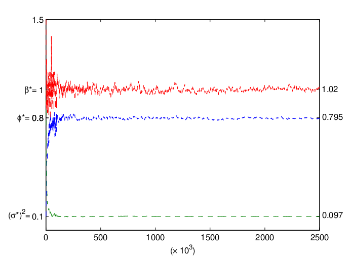
Figure 2 shows the parameter estimates obtained using the SMC implementation of online EM for the stochastic volatility model discussed in Example 4.1. The true value of the parameters were θ∗=(ϕ,σ2,β2)=(0.8,0.1,1)\theta^{\ast}=\left(\phi,\sigma^{2},\beta^{2}\right)=\left(0.8,0.1,1\right) and 500 particles were used. SMC-EM was started at the initial guess θ0=(0.1,1,2)\theta_{0}=(0.1,1,2). For the first 100 observations, only the E-step was executed. That is the step θn=Λ⁡(𝒮^n)\theta_{n}=\Lambda\left(\widehat{\mathcal{S}}_{n}\right), which is the M-step was skipped. SMC-EM was run in its entirety for observations 101 and onwards. The step size used was γn=0.01\gamma_{n}=0.01 for n≤105n\leq 10^{5} and 1/(n−  5×10⁴)0.61/(n-\,\,5\times 10^{4})^{0.6} for n>105n>10^{5}. Figure 2 shows the sequence of parameter estimates computed with a very long observation sequence.
Refer to caption
Figure 2: Estimating the parameters of the stochastic volatility model with the SMC version of online EM, Algorithm SMC-EM. Initial parameter guess θ0=(0.1,1,2)\theta_{0}=(0.1,1,2). True and converged values (average of the last 1000 iterations) are indicated on the left and the right of the plot respectively.

6 Discussion

We proposed a new SMC algorithm to compute the expectation of additive functionals recursively in time. Essentially, it is an online implementation of the FFBS SMC algorithm proposed in [18]. This algorithm has an 𝒪⁡(N2)\mathcal{O}(N^{2}) computational complexity where NN is the number of particles. It was mentioned how a standard path space SMC estimator to compute the same expectations recursively in time could be developed. This would have an 𝒪⁡(N)\mathcal{O}(N) computational complexity. However, as conjectured in [37], it was shown here that the asymptotic variance of the SMC-FFBS estimator increased linearly with time whereas that of the 𝒪⁡(N)\mathcal{O}(N) method increased quadratically. The online SMC-FFBS estimator was then used to perform recursive parameter estimation. While the convergence of RML and online EM have been established when they can be implemented exactly, the convergence of the SMC implementation of these algorithms have yet to be established and is currently under investigation.

7 Acknowledgments

The authors would like to thank Olivier Cappé, Thomas Flury, Sinan Yildirim and Éric Moulines for comments and references that helped improve the first version of this paper. The authors are also grateful to Rong Chen for pointing out the link between the forward smoothing recursion and dynamic programming. Finally, we are thankful to Robert Elliott to have pointed out to us references [22], [23] and [25].

Appendix A Appendix

The proofs in this section hold for any fixed θ\theta and therefore θ\theta is omitted from the notation. This section commences with some essential definitions.

Consider the measurable space (E,ℰ)(E,\mathcal{E}). Let ℳ⁡(E)\mathcal{M}(E) denote the set of all finite signed measures and 𝒫⁡(E)\mathcal{P}(E) the set of all probability measures on EE. Let ℬ⁡(E)\mathcal{B}(E) denote the Banach space of all bounded and measurable functions ff equipped with the uniform norm ‖f‖\|f\|. Let ν⁡(f)=∫ν⁡(𝑑x)​f​(x)\nu(f)=\int~\nu(dx)~f(x), i.e. ν⁡(f)\nu(f) is the Lebesgue integral of the function f∈ℬ⁡(E)f\in\mathcal{B}(E) w.r.t. the measure ν∈ℳ⁡(E)\nu\in\mathcal{M}(E). If ν\nu is a density w.r.t. some dominating measure d​xdx on EE then, ν⁡(f)=∫ν⁡(x)​f​(x)​𝑑x\nu(f)=\int\nu(x)~f(x)dx. We recall that a bounded integral kernel M⁡(x,d​x′)M(x,dx^{\prime}) from a measurable space (E,ℰ)(E,\mathcal{E}) into an auxiliary measurable space (E′,ℰ′)(E^{\prime},\mathcal{E}^{\prime}) is an operator f↦M⁡(f)f\mapsto M(f) from ℬ⁡(E′)\mathcal{B}(E^{\prime}) into ℬ⁡(E)\mathcal{B}(E) such that the functions

x↦M⁡(f)​(x):=∫E′M⁡(x,d​x′)​f​(x′)x\mapsto M(f)(x):=\int_{E^{\prime}}M(x,dx^{\prime})f(x^{\prime})

are ℰ\mathcal{E}-measurable and bounded, for any f∈ℬ⁡(E′)f\in\mathcal{B}(E^{\prime}). In the above displayed formulae, d​x′dx^{\prime} stands for an infinitesimal neighborhood of a point x′x^{\prime} in E′E^{\prime}. Let β⁡(M)\beta(M) denote the Dobrushin coefficient of MM which defined by the following formula

β⁡(M):=sup{osc​(M⁡(f));f∈Osc1​(E′)}\beta(M):=\sup{\ \{\mbox{\rm osc}(M(f))\;;\;\;f\in\mbox{\rm Osc}_{1}(E^{\prime})\}}

where Osc1​(E′)\mbox{Osc}_{1}(E^{\prime}) stands the set of ℰ′\mathcal{E^{\prime}}-measurable functions ff with oscillation less than or equal to 1. The kernel MM also generates a dual operator ν↦ν​M\nu\mapsto\nu M from ℳ⁡(E)\mathcal{M}(E) into ℳ⁡(E′)\mathcal{M}(E^{\prime}) defined by (ν​M)​(f):=ν​(M​(f))(\nu M)(f):=\nu(M(f)). A Markov kernel is a positive and bounded integral operator MM with M⁡(1)=1M(1)=1. Given a pair of bounded integral operators (M1,M2)(M_{1},M_{2}), we let (M1​M2)(M_{1}M_{2}) the composition operator defined by (M1​M2)​(f)=M1​(M2​(f))(M_{1}M_{2})(f)=M_{1}(M_{2}(f)). For time homogenous state spaces, we denote by Mm(=Mm−1M=MMm−1)M^{m}\,\left(=M^{m-1}M=MM^{m-1}\right) the mm-th composition of a given bounded integral operator MM, with m≥1m\geq 1.

Given a positive function GG on EE, let ΨG:ν∈𝒫⁡(E)↦ΨG​(ν)∈𝒫⁡(E)\Psi_{G}~:~\nu\in\mathcal{P}(E)\mapsto\Psi_{G}(\nu)\in\mathcal{P}(E) be the Bayes transformation defined by

ΨG​(ν)​(d​x):=1ν⁡(G)​G​(x)​ν​(d​x)\Psi_{G}(\nu)(dx):=\frac{1}{\nu(G)}~G(x)~\nu(dx)

The definitions above also apply if ν\nu is a density and MM is a transition density. In this case all instances of ν⁡(d​x)\nu(dx) should be replaced with ν⁡(x)​d​x\nu(x)dx and M⁡(x,d​x′)M(x,dx^{\prime}) by M⁡(x,x′)​d​x′M(x,x^{\prime})dx^{\prime} where d​xdx and d​x′dx^{\prime} are the dominating measures.

The proofs below will apply to any fixed sequence of observation {yn}n≥0\{y_{n}\}_{n\geq 0} and it is convenient to introduce the following transition kernels,

Qn​(xn−1,d​xn)\displaystyle Q_{n}(x_{n-1},dx_{n}) =g⁡(yn−1|xn−1)​f​(xn|xn−1)​d​xn,n≥1,\displaystyle=g(y_{n-1}|x_{n-1})f(x_{n}|x_{n-1})dx_{n},\quad n\geq 1,
andQk,n\displaystyle\mbox{\rm and}\quad Q_{k,n} =Qk+1​Qk+2​…​Qn,0≤k≤n,\displaystyle=Q_{k+1}Q_{k+2}\ldots Q_{n},\quad 0\leq k\leq n,

with the convention that Qn,n=I​dQ_{n,n}=Id, the identity operator. Note that Qk,n(1)=p(yk:n−1|xk)Q_{k,n}(1)=p(y_{k:n-1}|x_{k}).

Let the mapping Φk:𝒫⁡(𝒳)→𝒫⁡(𝒳)\Phi_{k}:\mathcal{P}(\mathcal{X})\rightarrow\mathcal{P}(\mathcal{X}), k≥1k\geq 1, be defined as follows

Φk​(ν)​(d​xk)=ν​Qk​(d​xk)ν​Qk​(1).\Phi_{k}(\nu)(dx_{k})=\frac{\nu Q_{k}(dx_{k})}{\nu Q_{k}(1)}.

Several probability densities and their SMC approximations are introduced to simplify the exposition. The predicted filter is denoted by

ηn(dxn)=p(dxn|y0:n−1)\eta_{n}(dx_{n})=p(dx_{n}\left|y_{0:n-1}\right.)

with the understanding that η0​(d​x0)\eta_{0}(dx_{0}) is the initial distribution of X0X_{0}. Let ηnN\eta_{n}^{N} denote its SMC approximation with NN particles. (This notation for the SMC approximation is opted for, instead of the usual η^n\widehat{\eta}_{n}, to make the number of particles explicit.) The bounded integral operator Dk,nD_{k,n} from 𝒳\mathcal{X} into 𝒳n+1\mathcal{X}^{n+1} is defined as

Dk,n(Sn)(xk):=∫p(dx0:k−1|xk,y0:k−1)(∏q=kn−1g(yq|xq)f(xq+1|xq))Sn(x0:n)dxk+1:nD_{k,n}(S_{n})(x_{k}):=\int p(dx_{0:k-1}\left|x_{k},y_{0:k-1}\right.)\left(\prod\limits_{q=k}^{n-1}g(y_{q}|x_{q})f(x_{q+1}|x_{q})\right)S_{n}(x_{0:n})dx_{k+1:n} (A.1)

Dk,nD_{k,n} is defined for any pair of time indices k,nk,n satisfying 0≤k≤n0\leq k\leq n with the convention that p(x0:k−1|xk,y0:k−1)=1p(x_{0:k-1}\left|x_{k},y_{0:k-1}\right.)=1 for k=0k=0 and ∏∅=1\prod\emptyset=1. The SMC approximation, Dk,nND_{k,n}^{N}, is

Dk,nN(Sn)(xk):=∫pN(dx0:k−1|xk,y0:k−1)(∏q=kn−1g(yq|xq)f(xq+1|xq))Sn(x0:n)dxk+1:nD_{k,n}^{N}(S_{n})(x_{k}):=\int p^{N}(dx_{0:k-1}\left|x_{k},y_{0:k-1}\right.)\left(\prod\limits_{q=k}^{n-1}g(y_{q}|x_{q})f(x_{q+1}|x_{q})\right)S_{n}(x_{0:n})dx_{k+1:n} (A.2)

where pN(dx0:k−1|xk,y0:k−1)p^{N}(dx_{0:k-1}\left|x_{k},y_{0:k-1}\right.) is the SMC approximation of p(dx0:k−1|xk,y0:k−1)p(dx_{0:k-1}\left|x_{k},y_{0:k-1}\right.) obtained from the SMC-FFBS approximation of Section 2.1, i.e.

pN(dx0:k−1|xk,y0:k−1)=∏q=1kMq,ηq−1N(xq,dxq−1)p^{N}(dx_{0:k-1}\left|x_{k},y_{0:k-1}\right.)=\prod\limits_{q=1}^{k}M_{q,\eta_{q-1}^{N}}(x_{q},dx_{q-1}) (A.3)

where the backward Markov transition kernels Mq,ηq−1NM_{q,\eta_{q-1}^{N}} are defined through

Mq,ηq−1N​(xq,d​xq−1)=ηq−1N​(d​xq−1)​g​(yq−1|xq−1)​f​(xq|xq−1)ηq−1N(g(yq−1|⋅)f(xq|⋅)).M_{q,\eta_{q-1}^{N}}(x_{q},dx_{q-1})=\frac{\eta_{q-1}^{N}(dx_{q-1})g(y_{q-1}|x_{q-1})f(x_{q}|x_{q-1})}{\eta_{q-1}^{N}(g(y_{q-1}|\cdot)f(x_{q}|\cdot))}. (A.4)

It is easily established that the SMC-FFBS approximation of p(dxk|y0:n)p(dx_{k}|y_{0:n}), k≤nk\leq n, is precisely the marginal of

pN(dx0:n−1|xn,y0:n−1)p^(dxn|y0:n)p^{N}(dx_{0:n-1}\left|x_{n},y_{0:n-1}\right.)\widehat{p}(dx_{n}|y_{0:n})

where p^(dxn|y0:n)\widehat{p}(dx_{n}|y_{0:n}) was defined in (1.9). Finally, we define

Pk,n=Dk,nDk,n​(1)andPk,nN=Dk,nNDk,nN​(1).P_{k,n}=\frac{D_{k,n}}{D_{k,n}(1)}\quad\text{and}\quad P_{k,n}^{N}=\frac{D_{k,n}^{N}}{D_{k,n}^{N}(1)}.

The following estimates are a straightforward consequence of Assumption (A). For time indices 0≤k≤q≤n0\leq k\leq q\leq n,

bk,n=supxk,xk′Qk,n​(1)​(xk)Qk,n​(1)​(xk′)≤ρ2​δ2,β⁡(Qk,q​(xk,d​xq)​Qq,n​(1)​(xq)Qk,q​(Qq,n​(1)))≤(1−ρ−4)(q−k),b_{k,n}=\sup_{x_{k},x_{k}^{\prime}}{\frac{Q_{k,n}(1)(x_{k})}{Q_{k,n}(1)(x_{k}^{\prime})}}\leq\rho^{2}\delta^{2},\quad\beta\left(\frac{Q_{k,q}(x_{k},dx_{q})Q_{q,n}(1)(x_{q})}{Q_{k,q}(Q_{q,n}(1))}\right)\leq\left(1-\rho^{-4}\right)^{(q-k)}, (A.5)

and for 0<k≤q0<k\leq q,

Mk,η​(x,d​z)≤ρ4​Mk,η​(x′,d​z)⟹β⁡(Mq,ηq−1N​…​Mk,ηk−1N)≤(1−ρ−4)q−k+1.M_{k,\eta}(x,dz)\leq\rho^{4}~M_{k,\eta}(x^{\prime},dz)\Longrightarrow\beta\left(M_{q,\eta_{q-1}^{N}}\ldots M_{k,\eta_{k-1}^{N}}\right)\leq\left(1-\rho^{-4}\right)^{q-k+1}. (A.6)

Several auxiliary results are now presented. For any φ∈ℬ⁡(𝒳)\varphi\in\mathcal{B}(\mathcal{X}), let

VkN​(φ)=ηkN​(φ)−Φk​(ηk−1N)​(φ).V_{k}^{N}(\varphi)=\eta_{k}^{N}(\varphi)-\Phi_{k}(\eta_{k-1}^{N})(\varphi). (A.7)

The following is an almost sure Kintchine type inequality [14, Lemma 7.3.3].

Lemma A.1

Let ℱnN:=σ({Xk(i);0≤k≤n,1≤i≤N,})\mathcal{F}_{n}^{N}:=\sigma\left(\left\{X_{k}^{(i)};0\leq k\leq n,1\leq i\leq N,\right\}\right), n≥0n\geq 0, be the natural filtration associated with the NN-particle approximation model and ℱ−1N\mathcal{F}_{-1}^{N} be the trivial sigma field. For any r≥1r\geq 1, there exist a finite (non random) constant ara_{r} such that the following inequality holds for all k≥0k\geq 0 and ℱk−1N\mathcal{F}_{k-1}^{N}\ measurable functions φkN∈ℬ⁡(𝒳)\varphi_{k}^{N}\in\mathcal{B}(\mathcal{X}) s.t. osc​(φkN)≤1\mbox{\rm osc}(\varphi_{k}^{N})\leq 1,

𝔼(|NVkN(φkN)|r|ℱk−1N)1r≤ar.\mathbb{E}\left(\left|\sqrt{N}V_{k}^{N}(\varphi_{k}^{N})\right|^{r}~\left|~\mathcal{F}_{k-1}^{N}\right.\right)^{\frac{1}{r}}\leq a_{r}.

This inequality may be used to derive the following 𝕃r\mathbb{L}_{r} error estimate [14, Theorem 7.4.4].

Lemma A.2

For any r≥1r\geq 1, there exists a constant ara_{r} such that the following inequality holds for all k≥0k\geq 0 and φ∈ℬ⁡(𝒳)\varphi\in\mathcal{B}(\mathcal{X}) s.t. osc​(φ)≤1\mbox{\rm osc}(\varphi)\leq 1,

N​𝔼​(|[ηnN−ηn]​(φ)|r)1r≤ar​∑k=0nbk,n​β​(Qk,nQk,n​(1)).\sqrt{N}\mathbb{E}\left(\left|[\eta_{n}^{N}-\eta_{n}](\varphi)\right|^{r}\right)^{\frac{1}{r}}\leq a_{r}~\sum_{k=0}^{n}~b_{k,n}~\beta\left(\frac{Q_{k,n}}{Q_{k,n}(1)}\right). (A.8)

A time-uniform bound for (A.8) may be obtained by using the estimates in (A.5)-(A.6). The final auxiliary result is the following.

Lemma A.3

For time indices 1≤k≤n1\leq k\leq n,

ηk−1N​Dk−1,nN​(Sn)=(ηk−1N​Qk)​(Dk,nN​(Sn))\eta_{k-1}^{N}D_{k-1,n}^{N}(S_{n})=(\eta_{k-1}^{N}Q_{k})(D_{k,n}^{N}(S_{n}))

Proof:

ηk−1N​Dk−1,nN​(Sn)=∫ηk−1N(dxk−1)pN(dx0:k−2|xk−1,y0:k−2)(∏q=knQq(xq−1,dxq))Sn(x0:n)=∫ηk−1N​(d​xk−1)​Qk​(xk−1,d​xk)×pN(dx0:k−2|xk−1,y0:k−2)(∏q=k+1nQq(xq−1,dxq))Sn(x0:n)\begin{array}[]{l}\eta_{k-1}^{N}D_{k-1,n}^{N}(S_{n})\\ =\int\eta_{k-1}^{N}(dx_{k-1})p^{N}(dx_{0:k-2}\left|x_{k-1},y_{0:k-2}\right.)\left(\prod\limits_{q=k}^{n}Q_{q}(x_{q-1},dx_{q})\right)S_{n}(x_{0:n})\\ =\int\eta_{k-1}^{N}(dx_{k-1})Q_{k}(x_{k-1},dx_{k})\\ \hskip 85.35826pt\times p^{N}(dx_{0:k-2}\left|x_{k-1},y_{0:k-2}\right.)\left(\prod\limits_{q=k+1}^{n}Q_{q}(x_{q-1},dx_{q})\right)S_{n}(x_{0:n})\end{array}

The result follows upon noting that

ηk−1N​(d​xk−1)​Qk​(xk−1,d​xk)=ηk−1N​Qk​(d​xk)​Mk,ηk−1N​(xk,d​xk−1).\eta_{k-1}^{N}(dx_{k-1})Q_{k}(x_{k-1},dx_{k})=\eta_{k-1}^{N}Q_{k}(dx_{k})~M_{k,\eta_{k-1}^{N}}(x_{k},dx_{k-1}).

To prove Theorem 3.1, the same semigroup techniques of [14, Section 7.4.3] are employed.

Proof:
The following decomposition is central

𝒮n^−𝒮n=∑0≤k≤n(ηkN​Dk,nN​(Sn)ηkN​Dk,nN​(1)−ηk−1N​Dk−1,nN​(Sn)ηk−1N​Dk−1,nN​(1))\widehat{\mathcal{S}_{n}}-\mathcal{S}_{n}=\sum_{0\leq k\leq n}\left(\frac{\eta_{k}^{N}D_{k,n}^{N}(S_{n})}{\eta_{k}^{N}D_{k,n}^{N}(1)}-\frac{\eta_{k-1}^{N}D_{k-1,n}^{N}(S_{n})}{\eta_{k-1}^{N}D_{k-1,n}^{N}(1)}\right)

with the convention that η−1N​D−1,nN=η0​(d​x0)​∏q=1nQq​(xq−1,d​xq)\eta_{-1}^{N}D_{-1,n}^{N}=\eta_{0}(dx_{0})\prod\limits_{q=1}^{n}Q_{q}(x_{q-1},dx_{q}), for k=0k=0. Lemma A.3 states that

ηk−1N​Dk−1,nN​(Sn)=(ηk−1N​Qk)​(Dk,nN​(Sn))\eta_{k-1}^{N}D_{k-1,n}^{N}(S_{n})=(\eta_{k-1}^{N}Q_{k})(D_{k,n}^{N}(S_{n}))

and therefore the decomposition can be also written as

𝒮n^−𝒮n=∑0≤k≤n(ηkN​Dk,nN​(Sn)ηkN​Dk,nN​(1)−Φk​(ηk−1N)​(Dk,nN​(Sn))Φk​(ηk−1N)​(Dk,nN​(1)))\widehat{\mathcal{S}_{n}}-\mathcal{S}_{n}=\sum_{0\leq k\leq n}\left(\frac{\eta_{k}^{N}D_{k,n}^{N}(S_{n})}{\eta_{k}^{N}D_{k,n}^{N}(1)}-\frac{\Phi_{k}(\eta_{k-1}^{N})(D_{k,n}^{N}(S_{n}))}{\Phi_{k}(\eta_{k-1}^{N})(D_{k,n}^{N}(1))}\right) (A.9)

with the convention Φ0​(η−1N)=η0\Phi_{0}(\eta_{-1}^{N})=\eta_{0}, for k=0k=0. Let

S~k,nN=Sn−Φk​(ηk−1N)​(Dk,nN​(Sn))Φk​(ηk−1N)​(Dk,nN​(1)).\widetilde{S}_{k,n}^{N}=S_{n}-\frac{\Phi_{k}(\eta_{k-1}^{N})(D_{k,n}^{N}(S_{n}))}{\Phi_{k}(\eta_{k-1}^{N})(D_{k,n}^{N}(1))}.

Then every term in the r.h.s. of (A.9) takes the following form

ηkN​Dk,nN​(S~k,nN)ηkN​Dk,nN​(1)=ηk​Qk,n​(1)ηkN​Qk,n​(1)×VkN​(D¯k,nN​(S~k,nN))\frac{\eta_{k}^{N}D_{k,n}^{N}(\widetilde{S}_{k,n}^{N})}{\eta_{k}^{N}D_{k,n}^{N}(1)}=\frac{\eta_{k}Q_{k,n}(1)}{\eta_{k}^{N}Q_{k,n}(1)}\times V_{k}^{N}\left(\overline{D}_{k,n}^{N}(\widetilde{S}_{k,n}^{N})\right) (A.10)

where the integral operators D¯k,nN\overline{D}_{k,n}^{N} are defined as follows,

D¯k,nN​(Sn)=Dk,nN​(Sn)ηk​Qk,n​(1).\overline{D}_{k,n}^{N}(S_{n})=\frac{D_{k,n}^{N}(S_{n})}{\eta_{k}Q_{k,n}(1)}.

Finally, using (A.9) and (A.10), 𝒮n^−𝒮n\widehat{\mathcal{S}_{n}}-\mathcal{S}_{n} is expressed as

N​(𝒮n^−𝒮n)=InN​(Sn)+RnN​(Sn)\sqrt{N}\left(\widehat{\mathcal{S}_{n}}-\mathcal{S}_{n}\right)=I_{n}^{N}(S_{n})+R_{n}^{N}(S_{n})

where the first order term is

InN​(Sn):=∑0≤k≤nN​VkN​(D¯k,nN​(S~k,nN))I_{n}^{N}(S_{n}):=\sum_{0\leq k\leq n}\sqrt{N}V_{k}^{N}\left(\overline{D}_{k,n}^{N}(\widetilde{S}_{k,n}^{N})\right)

and the second order remainder term is

RnN​(Sn):=∑0≤k≤n1ηkN​D¯k,n​(1)​N​(ηk−ηkN)​D¯k,n​(1)×VkN​(D¯k,nN​(S~k,nN)).R_{n}^{N}(S_{n}):=\sum_{0\leq k\leq n}\frac{1}{\eta_{k}^{N}\overline{D}_{k,n}(1)}\sqrt{N}\left(\eta_{k}-\eta_{k}^{N}\right)\overline{D}_{k,n}(1)\times V_{k}^{N}\left(\overline{D}_{k,n}^{N}(\widetilde{S}_{k,n}^{N})\right).

The non-asymptotic variance bound is based on the triangle inequality

𝔼⁡{N​(𝒮n^−𝒮n)2}≤(𝔼​{InN​(Sn)2}12+𝔼​{RnN​(Sn)2}12)2,\mathbb{E}\left\{N\left(\widehat{\mathcal{S}_{n}}-\mathcal{S}_{n}\right)^{2}\right\}\leq\left(\mathbb{E}\left\{I_{n}^{N}(S_{n})^{2}\right\}^{\frac{1}{2}}+\mathbb{E}\left\{R_{n}^{N}(S_{n})^{2}\right\}^{\frac{1}{2}}\right)^{2}, (A.11)

and bounds are derived below for the individual expressions on the right-hand side of this equation.  Using the fact that {VkN​(D¯k,nN​(S~k,nN))}0≤k≤n\left\{V_{k}^{N}\left(\overline{D}_{k,n}^{N}(\widetilde{S}_{k,n}^{N})\right)\right\}_{0\leq k\leq n} is zero mean and uncorrelated,

𝔼⁡(InN​(Sn)2)=∑0≤k≤nN​𝔼​{VkN​(D¯k,nN​(S~k,nN))2}.\mathbb{E}\left(I_{n}^{N}(S_{n})^{2}\right)=\sum_{0\leq k\leq n}N\mathbb{E}\left\{V_{k}^{N}\left(\overline{D}_{k,n}^{N}(\widetilde{S}_{k,n}^{N})\right)^{2}\right\}. (A.12)

The following results are needed to bound the right-hand side of (A.12). First, observe that Dk,nN​(1)=Qk,n​(1)D_{k,n}^{N}(1)=Q_{k,n}(1), and D¯k,nN​(1)=D¯k,n​(1)\overline{D}_{k,n}^{N}(1)=\overline{D}_{k,n}(1). Now using the decomposition,

D¯k,nN​(S~k,nN)​(xk)=D¯k,n​(1)​(xk)×∫[Pk,nN​(Sn)​(xk)−Pk,nN​(Sn)​(xk′)]​ΨQk,n​(1)​(Φk​(ηk−1N))​(d​xk′),\begin{array}[]{l}\overline{D}_{k,n}^{N}(\widetilde{S}_{k,n}^{N})(x_{k})\\ =\overline{D}_{k,n}(1)(x_{k})\times\int~\left[P_{k,n}^{N}(S_{n})(x_{k})-P_{k,n}^{N}(S_{n})(x_{k}^{\prime})\right]~\Psi_{Q_{k,n}(1)}(\Phi_{k}(\eta_{k-1}^{N}))(dx_{k}^{\prime}),\end{array}

it follows that

‖D¯k,nN​(S~k,nN)‖≤bk,n​osc​(Pk,nN​(Sn))\left\|\overline{D}_{k,n}^{N}(\widetilde{S}_{k,n}^{N})\right\|\leq b_{k,n}~\mbox{\rm osc}(P_{k,n}^{N}(S_{n})) (A.13)

For linear functionals of the form (3.1), it is easily checked that

Dk,nN​(Sn)=Qk,n​(1)​∑0≤q≤k[Mk,ηk−1N​…​Mq+1,ηqN]​(sq)+∑k<q≤nQk,q​(sq​Qq,n​(1))D_{k,n}^{N}(S_{n})=Q_{k,n}(1)~\sum_{0\leq q\leq k}\left[M_{k,\eta_{k-1}^{N}}\ldots M_{q+1,\eta_{q}^{N}}\right](s_{q})+\sum_{k<q\leq n}Q_{k,q}(s_{q}~Q_{q,n}(1))

with the convention Mk,ηk−1N​…​Mk+1,ηkN=I​dM_{k,\eta_{k-1}^{N}}\ldots M_{k+1,\eta_{k}^{N}}=Id, the identity operator, for q=kq=k. Recalling that Dk,nN​(1)=Qk,n​(1)D_{k,n}^{N}(1)=Q_{k,n}(1), we conclude that

Pk,nN​(Sn)=sk+∑0≤q<k[Mk,ηk−1N​…​Mq+1,ηqN]​(sq)+∑k<q≤nQk,q​(Qq,n​(1)​sq)Qk,q​(Qq,n​(1))P_{k,n}^{N}(S_{n})=s_{k}+\sum_{0\leq q<k}\left[M_{k,\eta_{k-1}^{N}}\ldots M_{q+1,\eta_{q}^{N}}\right](s_{q})+\sum_{k<q\leq n}\frac{Q_{k,q}(Q_{q,n}(1)~s_{q})}{Q_{k,q}(Q_{q,n}(1))}

and therefore

Pk,nN​(Sn)=∑0≤q<k[Mk,ηk−1N​…​Mq+1,ηqN]​(sq)+∑k≤q≤nQk,q​(Qq,n​(1)​sq)Qk,q​(Qq,n​(1))P_{k,n}^{N}(S_{n})=\sum_{0\leq q<k}\left[M_{k,\eta_{k-1}^{N}}\ldots M_{q+1,\eta_{q}^{N}}\right](s_{q})+\sum_{k\leq q\leq n}\frac{Q_{k,q}(Q_{q,n}(1)~s_{q})}{Q_{k,q}(Q_{q,n}(1))}

Thus,

osc​(Pk,nN​(Sn))≤∑0≤q<kβ⁡(Mk,ηk−1N​…​Mq+1,ηqN)​osc​(sq)+∑k≤q≤nβ⁡(Qk,q​(xk,d​xq)​Qq,n​(1)​(xq)Qk,q​(Qq,n​(1)))​osc​(sq)\begin{array}[]{l}\mbox{\rm osc}(P_{k,n}^{N}(S_{n}))\\ \leq\sum_{0\leq q<k}\beta\left(M_{k,\eta_{k-1}^{N}}\ldots M_{q+1,\eta_{q}^{N}}\right)\mbox{\rm osc}(s_{q})+\sum_{k\leq q\leq n}~\beta\left(\frac{Q_{k,q}(x_{k},dx_{q})Q_{q,n}(1)(x_{q})}{Q_{k,q}(Q_{q,n}(1))}\right)~\mbox{\rm osc}(s_{q})\end{array} (A.14)

Using the estimates in (A.5) and (A.6) for the contraction coefficients, and the estimate in (A.5) for bk,nb_{k,n}, it follows that there exists some finite (non random) constant cc such that the bound

‖D¯k,nN​(S~k,nN)‖≤c\left\|\overline{D}_{k,n}^{N}(\widetilde{S}_{k,n}^{N})\right\|\leq c (A.15)

holds for any pair of time indexes k,nk,n satisfying 0≤k≤n0\leq k\leq n, particle number NN and choice of functions {sk}0≤k≤n\{s_{k}\}_{0\leq k\leq n}. The desired bound for (A.14) is now obtained by combining this result with Lemma A.1:

𝔼⁡(InN​(Sn)2)\displaystyle\mathbb{E}\left(I_{n}^{N}(S_{n})^{2}\right) =∑0≤k≤nN​𝔼​(VkN​(D¯k,nN​(S~k,nN))2)\displaystyle=\sum_{0\leq k\leq n}N\mathbb{E}\left(V_{k}^{N}(\overline{D}_{k,n}^{N}(\widetilde{S}_{k,n}^{N}))^{2}\right)
≤d⁡(n+1)\displaystyle\leq d(n+1) (A.16)

where dd is a constant whose value does not depend on (n,N,Sn)(n,N,S_{n}).  Concerning the term 𝔼⁡{RnN​(Sn)2}\mathbb{E}\left\{R_{n}^{N}(S_{n})^{2}\right\} in (A.11).

𝔼​{RnN​(Sn)2}12\displaystyle\mathbb{E}\left\{R_{n}^{N}(S_{n})^{2}\right\}^{\frac{1}{2}} ≤∑0≤k≤n1N​𝔼​{[1ηkN​D¯k,n​(1)​N​(ηk−ηkN)​D¯k,n​(1)×N​VkN​(D¯k,nN​(S~k,nN))]2}12\displaystyle\leq\sum_{0\leq k\leq n}\frac{1}{\sqrt{N}}\mathbb{E}\left\{\left[\frac{1}{\eta_{k}^{N}\overline{D}_{k,n}(1)}\sqrt{N}\left(\eta_{k}-\eta_{k}^{N}\right)\overline{D}_{k,n}(1)\times\sqrt{N}V_{k}^{N}\left(\overline{D}_{k,n}^{N}(\widetilde{S}_{k,n}^{N})\right)\right]^{2}\right\}^{\frac{1}{2}}
≤∑0≤k≤n1N​bk,n​𝔼​{[N​(ηk−ηkN)​D¯k,n​(1)×N​VkN​(D¯k,nN​(S~k,nN))]2}12\displaystyle\leq\sum_{0\leq k\leq n}\frac{1}{\sqrt{N}}b_{k,n}\mathbb{E}\left\{\left[\sqrt{N}\left(\eta_{k}-\eta_{k}^{N}\right)\overline{D}_{k,n}(1)\times\sqrt{N}V_{k}^{N}\left(\overline{D}_{k,n}^{N}(\widetilde{S}_{k,n}^{N})\right)\right]^{2}\right\}^{\frac{1}{2}}
≤∑0≤k≤n1N​bk,n​𝔼​{[N​(ηk−ηkN)​D¯k,n​(1)]4}14\displaystyle\leq\sum_{0\leq k\leq n}\frac{1}{\sqrt{N}}b_{k,n}\mathbb{E}\left\{\left[\sqrt{N}\left(\eta_{k}-\eta_{k}^{N}\right)\overline{D}_{k,n}(1)\right]^{4}\right\}^{\frac{1}{4}}
×𝔼​{[N​VkN​(D¯k,nN​(S~k,nN))]4}14\displaystyle\times\mathbb{E}\left\{\left[\sqrt{N}V_{k}^{N}\left(\overline{D}_{k,n}^{N}(\widetilde{S}_{k,n}^{N})\right)\right]^{4}\right\}^{\frac{1}{4}}
≤1N​e​(n+1)\displaystyle\leq\frac{1}{\sqrt{N}}e(n+1) (A.17)

where ee is a constant whose value does not depend on (n,N,Sn)(n,N,S_{n}). The second line follows from (A.5) and the third by the Cauchy-Schwartz inequality. The final line was arrived at by the same reasoning used to derive bound (A.16) and Lemma A.2. The assertion of the theorem may be verified by substituting bounds (A.16) and (A.17) into (A.11).

It is possible to write

∑k=1nγk2∏i=k+1n(1−γi)2+∑k=2n∑i=1k−1γi2(1−γi+1)2⋯(1−γn)2\sum\limits_{k=1}^{n}\gamma_{k}^{2}\prod\limits_{i=k+1}^{n}(1-\gamma_{i})^{2}+\sum\limits_{k=2}^{n}\sum\limits_{i=1}^{k-1}\gamma_{i}^{2}(1-\gamma_{i+1})^{2}\cdots(1-\gamma_{n})^{2}

as the sum in (A.18) below.

Lemma A.4

Let α∈(0.5,1]\alpha\in(0.5,1] and γn=n−α\gamma_{n}=n^{-\alpha} for n>0n>0. Then

lim infn→∞γn2+∑i=1n−1(n+1−i)γi2(1−γi+1)2⋯(1−γn)2>0.\underset{n\rightarrow\infty}{\liminf}\quad\gamma_{n}^{2}+\sum_{i=1}^{n-1}(n+1-i)\gamma_{i}^{2}(1-\gamma_{i+1})^{2}\cdots(1-\gamma_{n})^{2}>0. (A.18)

Proof:
Let ⌊a⌋\left\lfloor a\right\rfloor denote the largest integer less than or equal to aa. Since the result is obvious for α=1\alpha=1, let α∈(0.5,1)\alpha\in(0.5,1).

γn2+∑i=⌊n/2⌋n−1(n+1−i)γi2(1−γi+1)2⋯(1−γn)2\displaystyle\gamma_{n}^{2}+\sum_{i=\left\lfloor n/2\right\rfloor}^{n-1}(n+1-i)\gamma_{i}^{2}(1-\gamma_{i+1})^{2}\cdots(1-\gamma_{n})^{2}
≥γn2+γn2​∑i=⌊n/2⌋n−1(n+1−i)​(1−γ⌊n/2⌋)2​(n−i)\displaystyle\geq\gamma_{n}^{2}+\gamma_{n}^{2}\sum_{i=\left\lfloor n/2\right\rfloor}^{n-1}(n+1-i)(1-\gamma_{\left\lfloor n/2\right\rfloor})^{2(n-i)}
=γn2​(∑j=1n+1−⌊n/2⌋j​λnj−1−1(1−λn)2)+γn2(1−λn)2\displaystyle=\gamma_{n}^{2}\left(\sum_{j=1}^{n+1-\left\lfloor n/2\right\rfloor}j\lambda_{n}^{j-1}-\frac{1}{(1-\lambda_{n})^{2}}\right)+\frac{\gamma_{n}^{2}}{(1-\lambda_{n})^{2}}

where λn=(1−γ⌊n/2⌋)2\lambda_{n}=(1-\gamma_{\left\lfloor n/2\right\rfloor})^{2} and

∑j>0j​λnj−1=1(1−λn)2.\sum_{j>0}j\lambda_{n}^{j-1}=\frac{1}{(1-\lambda_{n})^{2}}.

It may be verified that

limn→∞γn2(1−λn)2=2−2​α−2\lim_{n\rightarrow\infty}\frac{\gamma_{n}^{2}}{(1-\lambda_{n})^{2}}=2^{-2\alpha-2}

and

limn→∞γn2​∑j>n+1−⌊n/2⌋j​λnj−1=0.\lim_{n\rightarrow\infty}\gamma_{n}^{2}\sum_{j>n+1-\left\lfloor n/2\right\rfloor}j\lambda_{n}^{j-1}=0.

Hence the result follows.

References

  • [1] Andrieu, C., De Freitas, J.F.G. and Doucet, A. (1999). Sequential MCMC for Bayesian model selection. Proc. IEEE Workshop on Higher Order Statistics, 130–134.
  • [2] Andrieu, C., Doucet, A. and Holenstein, R. (2010). Particle Markov chain Monte Carlo (with discussion). J. Royal Statist. Soc. B, 72, 269-342.
  • [3] Andrieu, C., Doucet, A. and Tadić, V. B. (2005). On-line parameter estimation in general state-space models. Proc. 44th IEEE Conf. on Decision and Control, 332–337.
  • [4] Benveniste, A., Métivier, M. and Priouret, P. (1990). Adaptive Algorithms and Stochastic Approximation. New York: Springer-Verlag.
  • [5] Bertsekas, D. and Shreve, S.E. (1978) Stochastic Optimal Control: The Discrete-Time Case, Academic Press.
  • [6] Carpenter, J., Clifford, P. and Fearnhead, P. (1999). An improved particle filter for non-linear problems. IEE proceedings - Radar, Sonar and Navigation, 146, 2-7.
  • [7] Cappé, O., Moulines, É. and Rydén, T. (2005) Inference in Hidden Markov Models. New York: Springer-Verlag.
  • [8] Cappé, O. (2009). Online sequential Monte Carlo EM algorithm. Proc. IEEE Workshop on Statistical Signal Processing, Cardiff, UK.
  • [9] Cappé, O. (2009). Online EM algorithm for hidden Markov models. Available at http://arxiv.org/abs/0908.2359
  • [10] Cérou, F., Del Moral, P. and Guyader, A. (2008). A non asymptotic variance theorem for unnormalized Feynman-Kac particle models, Technical report INRIA-00337392. Available at http://hal.inria.fr/inria-00337392_v1/
  • [11] Chopin, N. (2004). Central limit theorem for sequential Monte Carlo and its application to Bayesian inference. Ann. Statist., 32, 2385-2411.
  • [12] Coquelin, P.A., Deguest, R. and Munos, R. (2009). Sensitivity analysis in HMMs with application to likelihood maximization. Proc. Conf. NIPS, Vancouver, Canada.
  • [13] Del Moral, P. and Doucet, A. (2003). On a class of genealogical and interacting Metropolis models. Lecture Notes in Mathematics 1832, Berlin: Springer-Verlag, 415-46.
  • [14] Del Moral, P. (2004). Feynman-Kac Formulae: Genealogical and Interacting Particle Systems with Applications. New York: Springer-Verlag.
  • [15] Del Moral, P., Doucet, A. and Singh. S.S. (2010). A backward particle interpretation of Feynman-Kac formulae. ESAIM: Math. Model. Num. Analy., 44, 947-975.
  • [16] Del Moral, P. and Guionnet, A. (2001). On the stability of interacting processes with applications to filtering and genetic algorithms. Ann. Inst. H. Poincaré Probab. Statist., 37, 155–194.
  • [17] Douc, R., Garivier, A., Moulines, E. and Olsson, J. (2011). Sequential Monte Carlo smoothing for general state space hidden Markov models. Ann. Applied Proba., to appear.
  • [18] Doucet, A., Godsill, S. J. and Andrieu, C. (2000). On sequential Monte Carlo sampling methods for Bayesian filtering. Statistics and Computing, 10, 197–208.
  • [19] Doucet, A., De Freitas, J.F.G. and Gordon N.J. (eds.) (2001). Sequential Monte Carlo Methods in Practice. New York: Springer-Verlag.
  • [20] Durbin, J. and Koopman, S.J. (2001). Time Series Analysis by State-Space Methods, Cambridge University Press.
  • [21] Elliott, R.J., Aggoun, L. and Moore, J.B. (1996). Hidden Markov Models: Estimation and Control, Springer-Verlag.
  • [22] Elliott, R.J., Ford, J.J. and Moore, J.B. (2000) On-line consistent estimation of hidden Markov models. Technical report, Department of Systems Engineering, Australian National University.
  • [23] Elliott, R.J., Ford, J.J. and Moore, J.B. (2002) On-line almost-sure parameter estimation for partially observed discrete-time linear systems with known noise characteristics. Intern. J. Adapt. Control Sig. Proc., 16, 435-453.
  • [24] Fearnhead, P. (2002). MCMC, sufficient statistics and particle filters. J. Comp. Graph. Statist., 11, 848–862.
  • [25] Ford, J.J. (1998). Adaptive hidden Markov model estimation and applications. PhD thesis, Department of Systems Engineering, Australian National University.
  • [26] Godsill, S.J., Doucet, A. and West, M. (2004). Monte Carlo smoothing for nonlinear time series. J. Amer. Stat. Assoc., 99, 156-168.
  • [27] Hernando, D., Valentino, C. and Cybenko, G. (2005) Efficient computation of the hidden Markov model entropy for a given observation sequence. IEEE Trans. Info. Theory, 51, 2681-2685.
  • [28] Kantas, N., Doucet, A., Singh, S.S. and Maciejowski, J.M. (2009). An overview of sequential Monte Carlo methods for parameter estimation in general state-space models. in Proceedings IFAC System Identification (SysId) Meeting.
  • [29] Kitagawa, G. and Sato, S. (2001). Monte Carlo smoothing and self-organising state-space model. In [19], 178–195. New York: Springer.
  • [30] Klaas, M., De Freitas, N. and Doucet, A. (2005). Toward practical N2N^{2} Monte Carlo: The marginal particle filter. Proc. Uncertainty in Artificial Intelligence, 308-15.
  • [31] Le Corff, S., Fort, G. and Moulines, E. (2010) Online expectation-maximization algorithm to solve the SLAM problem. Technical report , Telecom-ParisTech.
  • [32] Le Gland, F. and Mevel, M. (1997) Recursive identification in hidden Markov models, Proceedings of the 36th IEEE Conference on Decision and Control, 3468-3473.
  • [33] Mongillo, G. and Denève, S. (2008). Online learning with hidden Markov models. Neural Computation, 20, 1706-1716.
  • [34] Olsson, J., Cappé, O., Douc, R. and Moulines, E. (2008). Sequential Monte Carlo smoothing with application to parameter estimation in non-linear state space models. Bernoulli, 14, 155-179.
  • [35] Pitt, M.K. & Shephard, N. (1999). Filtering via simulation: auxiliary particle filter. J. Am. Statist. Ass., 94, 590-9.
  • [36] Poyiadjis, G. (2006) Particle methods for parameter estimation in general state-space models. PhD thesis, Cambridge University.
  • [37] Poyiadjis, G., Doucet, A. and Singh, S.S. (2011). Particle approximations of the score and observed information matrix in state-space models with application to parameter estimation. Biometrika, to appear.
  • [38] Storvik, G. (2002). Particle filters in state space models with the presence of unknown static parameters. IEEE. Trans. Signal Proc., 50:2, 281–289.
  • [39] Titterington, D.M. (1984) Recursive parameter estimation using incomplete data. J. Royal Statist. Soc. B, 46, 257-267.
  • [40] Zeitouni, O. and Dembo, A. (1988). Exact filters for the estimation of the number of transitions of finite-state continuous-time Markov processes. IEEE Trans. Inform. Theory, 34, 890-893.