跳到论文正文
W Papers独立论文阅读器 arXiv:1012.5347 论文正文 计算阅读时间 · 0%
引用这篇论文根据当前论文元数据生成,正式投稿前建议核对。


License: arXiv.org perpetual non-exclusive license
arXiv:1012.5347v2 [math.PR] 02 Sep 2011

Induced measures of simple random walks on Sierpinski graphs

Ting-Kam Leonard Wong Address: Department of Mathematics
The Chinese University of Hong Kong
Shatin, NT
Hong Kong.
Email address: tkwong@math.cuhk.edu.hk
Date: August 24, 2026
Abstract.

In [K], Kaimanovich defined an augmented rooted tree (X,E)(X,E) corresponding to the Sierpinski gasket KK, and showed that the Martin boundary of the simple random walk {Zn}\{Z_{n}\} on it is homeomorphic to KK. It is of interest to determine the hitting distributions v𝐱(⋅)=ℙ𝐱{limn→∞Zn∈⋅}v_{{\bf x}}(\cdot)={\mathbb{P}}_{{\bf x}}\{\lim_{n\rightarrow\infty}Z_{n}\in\cdot\} induced on KK. Using a reflection principle based on the symmetries of KK, we show that if the walk starts at the root of (X,E)(X,E), the hitting distribution is exactly the normalized Hausdorff measure μ\mu on KK. In particular, each v𝐱v_{{\bf x}}, 𝐱∈X{\bf x}\in X, is absolutely continuous with respect to μ\mu. This answers a question of Kaimanovich [K, Problem 4.14]. The argument can be generalized to other symmetric self-similar sets.

Key words and phrases: 
Hyperbolic boundary, Martin boundary, simple random walk, Sierpinski gasket
1991 Mathematics Subject Classification
Primary: 60J10, 28A80; Secondary: 60J50.

1. Introduction

In [DS1], Denker and Sato constructed a transient Markov chain and showed that its Martin boundary can be identified as the Sierpinski gasket. This opened a new direction to study analysis on fractals via the boundary theory of random walk ([DS2], [DS3], [JLW], [K], [Ki], [LN], [LW1], [LW2], [P], [WL]). The key idea is to realize a fractal as the boundary of a random walk or graph; the potential theory associated with the discrete system is used to induce on the fractal objects such as harmonic measures, harmonic functions, and Dirichlet forms.

There are several ways to construct the random walks, and they are all related to the symbolic space of the underlying iterated function system. In [DS1], the transition function is one-way and gives rise to a reducible chain. This allows the Green function and Martin kernels be estimated explicitly. This construction was generalized to a class of p.c.f. fractals in [JLW] and in a more general setting in [LW2]. Also see [LN] for an interesting way of assigning probabilities where the minimal Martin boundary is a proper subset of the Martin boundary.

Another approach was provided by Kaimanovich [K], who introduced an augmented rooted tree (which he also called the Sierpinski graph) to realize the Sierpinski gasket as a hyperbolic boundary in the sense of Gromov [G]. Moreover, he showed that the simple random walk on the graph has a Martin boundary homeomorphic to the Sierpinski gasket. The augmented rooted tree was generalized in [LW1] to cover all iterated function systems satisfying the open set condition (OSC), and it was shown in [WL] that for strictly reversible random walks the Martin boundary coincides with the hyperbolic boundary, which is the self-similar set.

Refer to caption
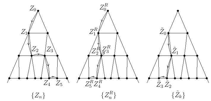
Figure 1. The simple random walk {Zn}\{Z_{n}\} on (X,E)(X,E) induces a family of hitting distributions on the Sierpinski gasket.

The random walk induces naturally a family of hitting distributions, or harmonic measures, on the self-similar set. The purpose of this paper is to study these induced measures for the simple random walk on the Sierpinski graphs in [K]. The main problem is to determine whether the measures are absolutely continuous with respect to the Hausdorff or a self-similar measure. Apart from its probabilistic interest, this question is important as the hitting distribution from the root serves as the reference measure of the induced Dirichlet form constructed in [WL] (also see [Ki] for the case of Cantor sets).

Our main result answers a question of Kaimanovich [K, Problem 4.14].

Theorem 1.1.

Consider the simple random walk {Zn}\{Z_{n}\} on the augmented rooted tree (X,E)(X,E) corresponding to the Sierpinski gasket KK in ℝd{\mathbb{R}}^{d}, d≥1d\geq 1. Let Z∞=limnZnZ_{\infty}=\lim_{n}Z_{n} be the limit of the walk on KK and let νϑ(⋅)=ℙϑ{Z∞∈⋅}\nu_{\vartheta}(\cdot)={\mathbb{P}}_{\vartheta}\{Z_{\infty}\in\cdot\} be the hitting distribution where the starting point is the root ϑ\vartheta. Then νϑ\nu_{\vartheta} equals the normalized α\alpha-dimensional Hausdorff measure μ\mu on KK, where α=dimHK\alpha=\dim_{H}K.

Since {Zn}\{Z_{n}\} is irreducible, we immediately get the following (see [Wo, p. 221]).

Corollary 1.2.

For all 𝐱∈X{\bf x}\in X, the hitting distribution ν𝐱(⋅)=ℙ𝐱{Z∞∈⋅}\nu_{{\bf x}}(\cdot)={\mathbb{P}}_{{\bf x}}\{Z_{\infty}\in\cdot\} is absolutely continuous with respect to μ\mu.

The main obstacle is that ZnZ_{n} can travel not only up and down but also through the horizontal edges. This makes it very difficult to estimate the transition probabilities and the Martin kernels. Instead of estimating them, we shall exploit the symmetries of the Sierpinski gasket and prove directly that νϑ\nu_{\vartheta} satisfies two identities which we call the group invariance identity (Theorem 3.5) and the self-similar identity (Theorem 5.5). They force νϑ\nu_{\vartheta} to be exactly μ\mu. The argument involves interesting probabilistic and algebraic constructions. Our method can be generalized to some other symmetric self-similar sets, but for simplicity we restrict ourselves to the case of Sierpinski gaskets.

This paper is organized as follows. In Section 2, we review the construction of the Sierpinski graph (X,E)(X,E) and identify the Sierpinski gasket as the Martin boundary of the simple random walk {Zn}\{Z_{n}\} on (X,E)(X,E). For motivation, we also give a heuristic argument for the simplest case of dimension 11, where the boundary is simply a unit interval. To generalize the argument to higher dimensions, in Section 3 we analyze the symmetries of the Sierpinski gasket and their actions on (X,E)(X,E). They are used to formulate the group invariance identity. In Section 4 we introduce a reflection principle and construct a coupling of {Zn}\{Z_{n}\} with a simple random walk {Z~k}\{\tilde{Z}_{k}\} on the subgraph 0​X0X which is isomorphic to XX. This is used in Section 5 to prove the self-similar identity and the main theorem. Section 6 contains further remarks, including extension to other symmetric self-similar sets, and some open questions.

2. Preliminaries and motivations

In this section we introduce the notations and identify the Sierpinski gasket as a Martin boundary. The reader can refer to [WL] for a detailed treatment under a more general setting. Fix d≥1d\geq 1 and a collection of points {pi}i=0d\{p_{i}\}_{i=0}^{d} that generates a regular simplex in ℝd{\mathbb{R}}^{d}, i.e., |pi−pj|=δi​j|p_{i}-p_{j}|=\delta_{ij}. The dd-dimensional Sierpinski gasket, denoted by K=KdK=K^{d}, is the self-similar set of the iterated function system (IFS) Fi​(x)=12​pi+12​xF_{i}(x)=\frac{1}{2}p_{i}+\frac{1}{2}x, i=0,…,di=0,...,d.

Following [K] and [LW1], we define an augmented rooted tree (or Sierpinski graph) (X,E)(X,E) as follows. Let

X={ϑ}∪⋃n=1∞{0,1,…,d}nX=\{\vartheta\}\cup\bigcup_{n=1}^{\infty}\{0,1,...,d\}^{n}

be the symbolic space corresponding to the IFS {Fi}i=0d\{F_{i}\}_{i=0}^{d}. Here ϑ\vartheta is the empty word which will be regarded as the root of (X,E)(X,E). For 𝐱=i1​…​in∈X{\bf x}=i_{1}...i_{n}\in X, we let |𝐱|=n|{\bf x}|=n be the length of 𝐱{\bf x} and define F𝐱=Fi1∘⋯∘SinF_{{\bf x}}=F_{i_{1}}\circ\cdots\circ S_{i_{n}} (we define Sϑ=idS_{\vartheta}=\mathrm{id} by convention). We let K𝐱=F𝐱​(K)K_{{\bf x}}=F_{{\bf x}}(K) be the cell corresponding to 𝐱∈X{\bf x}\in X. If 𝐱=i1​…​in∈X∖{ϑ}{\bf x}=i_{1}...i_{n}\in X\setminus\{\vartheta\}, we use 𝐱−=i1​…​in−1{\bf x}^{-}=i_{1}...i_{n-1} to denote the ancestor of 𝐱{\bf x}.

The edge set E=Ev∪EhE=E_{v}\cup E_{h} of the Sierpinski graph consists of vertical edges (Ev)(E_{v}) and horizontal edges (Eh)(E_{h}). We define, for 𝐱≠𝐲{\bf x}\neq{\bf y},

(𝐱,𝐲)∈Ev⇔𝐲=𝐱−​ or ​𝐱=𝐲−,(𝐱,𝐲)∈Eh⇔|𝐱|=|𝐲|​ and ​F𝐱​(K)∩F𝐲​(K)≠∅.\begin{array}[]{lllll}({\bf x},{\bf y})\in E_{v}&\Leftrightarrow&{\bf y}={\bf x}^{-}\text{ or }{\bf x}={\bf y}^{-},\\ ({\bf x},{\bf y})\in E_{h}&\Leftrightarrow&|{\bf x}|=|{\bf y}|\text{ and }F_{{\bf x}}(K)\cap F_{{\bf y}}(K)\neq\emptyset.\end{array}

We write 𝐱∼𝐲{\bf x}\sim{\bf y} if (𝐱,𝐲)∈E({\bf x},{\bf y})\in E. By a path in (X,E)(X,E), we mean a finite sequence {𝐱n}n=0N\{{\bf x}_{n}\}_{n=0}^{N} such that 𝐱n∼𝐱n+1{\bf x}_{n}\sim{\bf x}_{n+1} for all nn.

Refer to caption
Figure 2. The Sierpinski graphs corresponding to d=1d=1 (left) and d=2d=2 (right).

For 𝐱=i1​i2​…​in≠ϑ{\bf x}=i_{1}i_{2}...i_{n}\neq\vartheta, let p𝐱=Fi1​i2​…​in−1​(pin)p_{{\bf x}}=F_{i_{1}i_{2}...i_{n-1}}(p_{i_{n}}) be the ‘dyadic point’ on KK corresponding to 𝐱{\bf x}. In particular, for i≠ji\neq j,

pi​j=pj​i=Fi​(pj)=Fj​(pi)=12​pi+12​pjp_{ij}=p_{ji}=F_{i}(p_{j})=F_{j}(p_{i})=\frac{1}{2}p_{i}+\frac{1}{2}p_{j}

is the midpoint of the line segment [pi,pj][p_{i},p_{j}].

Let {Zn}\{Z_{n}\} be the simple random walk on (X,E)(X,E) with transition function PP, i.e.,

P⁡(𝐱,𝐲)={1deg⁡(𝐱),if 𝐱∼𝐲,0,otherwise.P({\bf x},{\bf y})=\left\{\begin{array}[]{ll}\frac{1}{{\mathrm{deg}}({\bf x})},&\hbox{if ${\bf x}\sim{\bf y}$,}\\ 0,&\hbox{otherwise.}\end{array}\right.

Here deg⁡(𝐱){\mathrm{deg}}({\bf x}), the degree of 𝐱{\bf x}, is the number of edges connecting 𝐱{\bf x}. The Green function of the walk is defined by

G⁡(𝐱,𝐲)=∑n=0∞Pn​(𝐱,𝐲),𝐱,𝐲∈X.G({\bf x},{\bf y})=\sum_{n=0}^{\infty}P^{n}({\bf x},{\bf y}),\ \ \ {\bf x},{\bf y}\in X.

Here PnP^{n} is the nn-step transition function. The Martin kernel is defined by

K⁡(𝐱,𝐲)=G⁡(𝐱,𝐲)G⁡(ϑ,𝐲),𝐱,𝐲∈X.K({\bf x},{\bf y})=\frac{G({\bf x},{\bf y})}{G(\vartheta,{\bf y})},\ \ \ {\bf x},{\bf y}\in X.

The Martin compactification of the random walk is defined as the minimal compactification X^\widehat{X} of XX such that for each 𝐱∈X{\bf x}\in X, the function K⁡(𝐱,⋅)K({\bf x},\cdot) extends continuously up to the Martin boundary ℳ=X^∖X{\mathcal{M}}=\widehat{X}\setminus X (see [Wo]). It can be shown that under the Martin topology, ZnZ_{n} converges almost surely to a point Z∞Z_{\infty} on the Martin boundary ℳ{\mathcal{M}}.

The following result first appeared as [K, Theorem 4.7] and is a special case of [WL, Theorem 3.5].

Theorem 2.1.

The Martin boundary of {Zn}\{Z_{n}\} is homeomorphic to the Sierpinski gasket KK under a canonical homeomorphism.

Hence, we may identify ℳ{\mathcal{M}} with KK and it makes sense to talk about the limit Z∞Z_{\infty} on KK. Following [WL], we may express the limit in terms of a projection ι:X→K\iota:X\rightarrow K. For any 𝐱∈X{\bf x}\in X, pick an arbitrary point ι⁡(𝐱)∈K𝐱\iota({\bf x})\in K_{{\bf x}}. Then under the usual topology of ℝd{\mathbb{R}}^{d}, we have

Z∞=limn→∞ι⁡(Zn).\displaystyle Z_{\infty}=\lim_{n\rightarrow\infty}\iota(Z_{n}). (2.1)

For example, when d=1d=1 and [p0,p1]=[0,1][p_{0},p_{1}]=[0,1], the sequence

ϑ,0,00,001,0011,00111,001111,…\vartheta,0,00,001,0011,00111,001111,...

converges to 14\frac{1}{4}.

The constructions in this paper involves some technicalities. To illustrate the main ideas, we give a heuristic argument for the case d=1d=1, where K1=[p0,p1]K^{1}=[p_{0},p_{1}] is simply a unit interval, say [0,1][0,1]. First, from the symmetry of (X,E)(X,E) and [0,1][0,1], we see that νϑ\nu_{\vartheta} must be symmetric about 12\frac{1}{2}:

νϑ​(B)=νϑ​(1−B)=νϑ​(R​B),B⊂[0,1]​ Borel.\displaystyle\nu_{\vartheta}(B)=\nu_{\vartheta}(1-B)=\nu_{\vartheta}(RB),\ \ \ B\subset[0,1]\ \text{ Borel}. (2.2)

Here R​x=1−xRx=1-x is the reflection about 12\frac{1}{2} and is a symmetry of [0,1][0,1]. We call (2.2) a group invariance identity.

Next, we observe that the subgraph 0​X={0​𝐱:𝐱∈X}0X=\{0{\bf x}:{\bf x}\in X\} is isomorphic to XX. We will use {Zn}\{Z_{n}\}, starting at ϑ\vartheta, to construct a simple random walk {Z~k}\{\tilde{Z}_{k}\} on 0​X0X starting at 00. The reflection RR induces naturally a reflection, also denoted by RR, on XX which flips all the symbols. For example, R​ϑ=ϑR\vartheta=\vartheta and R⁡(00101)=11010R(00101)=11010. Consider the reflected random walk {ZnR}\{Z^{R}_{n}\} defined by

ZnR={Zn,if Zn∈{ϑ}∪0​XR​Zn,if Zn∈1​X,n≥0.Z^{R}_{n}=\left\{\begin{array}[]{ll}Z_{n},&\hbox{if $Z_{n}\in\{\vartheta\}\cup 0X$}\\ RZ_{n},&\hbox{if $Z_{n}\in 1X$}\end{array}\right.,\ \ \ n\geq 0.
Refer to caption
Figure 3. The transformation {Zn}↦{Z~k}\{Z_{n}\}\mapsto\{\tilde{Z}_{k}\}

Note that ZnRZ^{R}_{n} always belongs to {ϑ}∪0​X\{\vartheta\}\cup 0X. Now we change time to skip the visits of ZnRZ^{R}_{n} to ϑ\vartheta and then look at the jump chain (see [N]). The resulting process has the form Z~k=ZTkR\tilde{Z}_{k}=Z^{R}_{T_{k}} where {Tk}\{T_{k}\} are suitable stopping times. It can be verified that {Z~k}\{\tilde{Z}_{k}\} is the simple random walk on 0​X0X starting at 00.

Since {Z~k}\{\tilde{Z}_{k}\} is a simple random walk on 0​X0X, it converges to some point Z~∞\tilde{Z}_{\infty} in [0,12][0,\frac{1}{2}]. Moreover, Z~k\tilde{Z}_{k} converges to a point x∈[0,12]x\in[0,\frac{1}{2}] if and only if the original walk ZnZ_{n} converges to either xx or 1−x=R​x1-x=Rx. It follows that

ℙϑ{Z~∞∈B}=ℙϑ{Z∞∈B∪RB},B⊂[0,12].{\mathbb{P}}_{\vartheta}\{\tilde{Z}_{\infty}\in B\}={\mathbb{P}}_{\vartheta}\{Z_{\infty}\in B\cup RB\},\ \ \ B\subset[0,\frac{1}{2}].
Refer to caption
Figure 4. Graphical illustration of the identities

On the other hand, [0,12][0,\frac{1}{2}] can be identified naturally with [0,1][0,1], and we get ℙϑ{Z~∞∈B}=ℙϑ{Z∞∈2B}=νϑ(2B){\mathbb{P}}_{\vartheta}\{\tilde{Z}_{\infty}\in B\}={\mathbb{P}}_{\vartheta}\{Z_{\infty}\in 2B\}=\nu_{\vartheta}(2B). Hence we obtain the following self-similar identity:

νϑ​(2​B)=νϑ​(B∪R​B),B⊂[0,12]​ Borel.\displaystyle\nu_{\vartheta}(2B)=\nu_{\vartheta}(B\cup RB),\ \ \ B\subset[0,\frac{1}{2}]\ \text{ Borel}. (2.3)

Now (2.2) and (2.3) imply that νϑ\nu_{\vartheta} is the Lebesgue measure on [0,1][0,1]. One way to prove this is to show inductively that νϑ​(I)\nu_{\vartheta}(I) equals the Lebesgue measure of II where II is any dyadic interval.

We will now generalize this idea to the Sierpinski gasket of abitrary dimension. We begin by analyzing the symmetries of the dd-dimensional Sierpinski gasket KdK^{d} in relation to the augmented rooted tree (X,E)(X,E).

3. Symmetries and group invariance identity

Let 𝒜d{\mathcal{A}}_{d} be the symmetry group of the dd-dimensional Sierpinski gasket K=Kd⊂ℝdK=K^{d}\subset{\mathbb{R}}^{d}, i.e., 𝒜d{\mathcal{A}}_{d} consists of those isometries on ℝd{\mathbb{R}}^{d} that fix KK. The next lemma is standard.

Lemma 3.1.

𝒜d{\mathcal{A}}_{d} is isomorphic to the symmetric group 𝒮d+1{\mathcal{S}}_{d+1} of d+1d+1 symbols. For each g∈𝒜dg\in{\mathcal{A}}_{d}, define gK:{0,…,d}→{0,…,d}g_{K}:\{0,...,d\}\rightarrow\{0,...,d\} by

gK​i=j if ​g​pi=pj.g_{K}i=j\ \ \text{ if }gp_{i}=p_{j}.

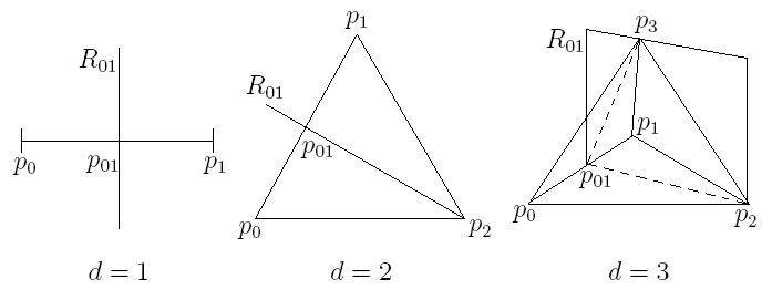
Then gK∈Sd+1g_{K}\in S_{d+1}, and g↦gKg\mapsto g_{K} is an isomorphism. We will identify gg and gKg_{K}. Moreover, the transformation Ri​j∈𝒜dR_{ij}\in{\mathcal{A}}_{d} corresponding to the transposition (i,j)(i,j) in 𝒮d+1{\mathcal{S}}_{d+1} is a reflection in ℝd{\mathbb{R}}^{d}. By convention, we set Ri​i=i​dR_{ii}=id.

Example 3.2.

We illustrate the reflection R01R_{01} on KdK^{d} where d≤3d\leq 3.

Refer to caption
Figure 5. The reflection R01R_{01}

We let Aut⁡(X)\mathrm{Aut}(X) be the automorphism group of (X,E)(X,E), i.e.

Aut(X)={φ:X→X|φ is bijective and 𝐱∼𝐲⇔φ(𝐱)∼φ(𝐲)}.\mathrm{Aut}(X)=\{\varphi:X\rightarrow X|\varphi\text{ is bijective and }{\bf x}\sim{\bf y}\Leftrightarrow\varphi({\bf x})\sim\varphi({\bf y})\}.

Each g∈𝒜dg\in{\mathcal{A}}_{d} also induces an element of Aut⁡(X)\mathrm{Aut}(X) via its action on the cells K𝐱K_{{\bf x}}.

Lemma 3.3.

For g∈𝒜dg\in{\mathcal{A}}_{d}, define gX:X→Xg_{X}:X\rightarrow X by

gX​𝐱=𝐲,if ​g​(K𝐱)=K𝐲.g_{X}{\bf x}={\bf y},\ \ \text{if }g(K_{{\bf x}})=K_{{\bf y}}.

Then gX∈Aut⁡(X)g_{X}\in\mathrm{Aut}(X), and g↦gXg\mapsto g_{X} is an injective homomorphism. We will identify gg and gXg_{X}. Moreover, PP is invariant under gg: for all g∈𝒜dg\in{\mathcal{A}}_{d} and 𝐱,𝐲∈X{\bf x},{\bf y}\in X,

P⁡(𝐱,𝐲)=P⁡(g​𝐱,g​𝐲).P({\bf x},{\bf y})=P(g{\bf x},g{\bf y}).
Proof.

The first part is standard. To see the second part, note that if 𝐱∼𝐲{\bf x}\sim{\bf y}, then g​𝐱∼g​𝐲g{\bf x}\sim g{\bf y} and

P⁡(𝐱,𝐲)=1deg⁡(𝐱)=1deg⁡(g​𝐱)=P⁡(g​𝐱,g​𝐲).P({\bf x},{\bf y})=\frac{1}{{\rm deg}({\bf x})}=\frac{1}{{\rm deg}(g{\bf x})}=P(g{\bf x},g{\bf y}).

And if 𝐱≁𝐲{\bf x}\nsim{\bf y} then both sides are 00. ∎

The next lemma says that g∈𝒜dg\in{\mathcal{A}}_{d} and g∈Aut⁡(X)g\in\mathrm{Aut}(X) commute in the limit.

Lemma 3.4.

For any Borel set BB in KK and g∈𝒜dg\in{\mathcal{A}}_{d},

{Z∞∈B}={gZ∞∈gB}={limn→∞(gZn)∈gB}.\{Z_{\infty}\in B\}=\{gZ_{\infty}\in gB\}=\{\lim_{n\rightarrow\infty}(gZ_{n})\in gB\}.
Proof.

Let g∈𝒜dg\in{\mathcal{A}}_{d} be given. By Lemma 3.3, ι⁡(g​𝐱)∈Kg​𝐱=g⁡(K𝐱)\iota(g{\bf x})\in K_{g{\bf x}}=g(K_{{\bf x}}) for all 𝐱∈X{\bf x}\in X. It follows that

|ι⁡(g​Zn)−g​ι​(Zn)|≤diam⁡(KZn)→0|\iota(gZ_{n})-g\iota(Z_{n})|\leq\mathrm{diam}(K_{Z_{n}})\rightarrow 0

as |Zn|→∞|Z_{n}|\rightarrow\infty. Suppose Z∞=yZ_{\infty}=y. Then ι⁡(Zn)→y\iota(Z_{n})\rightarrow y and |Zn|→∞|Z_{n}|\rightarrow\infty imply that

|ι⁡(g​Zn)−g​y|≤|ι⁡(g​Zn)−g​ι​(Zn)|+|g​ι​(Zn)−g​y|→0|\iota(gZ_{n})-gy|\leq|\iota(gZ_{n})-g\iota(Z_{n})|+|g\iota(Z_{n})-gy|\rightarrow 0

as n→∞n\rightarrow\infty. It follows that g​Zn→g​ygZ_{n}\rightarrow gy. Similarly, limng​Zn=g​y\lim_{n}gZ_{n}=gy implies that Z∞=yZ_{\infty}=y. ∎

Theorem 3.5.

(Group invariance identities) The hitting distribution νϑ(⋅)=ℙϑ{Z∞∈⋅}\nu_{\vartheta}(\cdot)={\mathbb{P}}_{\vartheta}\{Z_{\infty}\in\cdot\} is invariant under the action of 𝒜d{\mathcal{A}}_{d}, i.e., for any Borel set BB in KK,

νϑ​(B)=νϑ​(g​B),g∈𝒜d.\nu_{\vartheta}(B)=\nu_{\vartheta}(gB),\ \ \ g\in{\mathcal{A}}_{d}.
Proof.

Fix g∈𝒜dg\in{\mathcal{A}}_{d}. By Lemma 3.3, the processes {g​Zn}\{gZ_{n}\} and {Zn}\{Z_{n}\} have the same finite dimensional distributions under ℙϑ{\mathbb{P}}_{\vartheta}. It follows by a monotone class argument that limn→∞g​Zn\lim_{n\rightarrow\infty}gZ_{n} and Z∞Z_{\infty} have the same distribution under ℙϑ{\mathbb{P}}_{\vartheta} as well.

Let BB be a Borel set in KK. Then

νϑ​(g​B)\displaystyle\nu_{\vartheta}(gB) =\displaystyle= ℙϑ{Z∞∈gB}\displaystyle{\mathbb{P}}_{\vartheta}\{Z_{\infty}\in gB\} (3.1)
=\displaystyle= ℙϑ{g−1Z∞∈B}\displaystyle{\mathbb{P}}_{\vartheta}\{g^{-1}Z_{\infty}\in B\}
=\displaystyle= ℙϑ{limn→∞(g−1Zn)∈B}\displaystyle{\mathbb{P}}_{\vartheta}\{\lim_{n\rightarrow\infty}(g^{-1}Z_{n})\in B\}
=\displaystyle= ℙϑ{Z∞∈B}\displaystyle{\mathbb{P}}_{\vartheta}\{Z_{\infty}\in B\} (3.2)
=\displaystyle= νϑ​(B).\displaystyle\nu_{\vartheta}(B).

In the above, (3.1) follows from Lemma 3.4, and (3.2) follows from the fact that limn→∞g​Zn\lim_{n\rightarrow\infty}gZ_{n} and Z∞Z_{\infty} have the same distribution. ∎

4. Reflection principle

In this section we construct the process {Z~k}\{\tilde{Z}_{k}\} by repeated reflections and show that it is a simple random walk on 0​X0X. We use Ω\Omega to denote the sample space consisting of all sample paths ω\omega such that Zn+1​(ω)∼Zn​(ω)Z_{n+1}(\omega)\sim Z_{n}(\omega) for all nn (note that the simple random walk is of the nearest-neighbor type). For simplicity, we restrict the starting point to be ϑ\vartheta, and we will work under ℙϑ{\mathbb{P}}_{\vartheta}. With slight modification the starting point can be arbitrary.

First we introduce some notations. For 𝐱∈X∖{ϑ}{\bf x}\in X\setminus\{\vartheta\}, we define the parity [𝐱][{\bf x}] of 𝐱{\bf x} as the first symbol of 𝐱{\bf x}. That is, if 𝐱=i1​i2​…​in{\bf x}=i_{1}i_{2}...i_{n}, then [𝐱]=i1[{\bf x}]=i_{1}. By convention, we set [ϑ]=0[\vartheta]=0. For 𝐱∈X{\bf x}\in X, we define a set 𝒩𝐱{\mathcal{N}}_{{\bf x}} by

𝒩𝐱={{j:j≠i},𝐱=i,{j​im−1},𝐱=i​jm−1,i≠j,m≥2,∅,otherwise.{\mathcal{N}}_{{\bf x}}=\left\{\begin{array}[]{ll}\{j:j\neq i\},&\hbox{${\bf x}=i$,}\\ \{ji^{m-1}\},&\hbox{${\bf x}=ij^{m-1},i\neq j,\ m\geq 2$,}\\ \emptyset,&\hbox{otherwise.}\end{array}\right.

In words, 𝐲∈𝒩𝐱{\bf y}\in{\mathcal{N}}_{{\bf x}} if the parity changes when the walk jumps from 𝐱{\bf x} to 𝐲{\bf y} horizontally (𝒩{\mathcal{N}} stands for neighbor).

For technical convenience, we will first change the time of {Zn}\{Z_{n}\}. Let {ℱn}\{{\mathcal{F}}_{n}\} be the standard filtration of {Zn}\{Z_{n}\}. We define a strictly increasing sequence of {ℱn}\{{\mathcal{F}}_{n}\}-stopping times {Tk}k≥0\{T_{k}\}_{k\geq 0} by

T0\displaystyle T_{0} =\displaystyle= inf{n≥0:Zn≠ϑ},\displaystyle\inf\{n\geq 0:Z_{n}\neq\vartheta\},
Tk+1\displaystyle T_{k+1} =\displaystyle= inf{n>Tk:Zn∉{ZTk}∪{ϑ}∪𝒩ZTk},k≥0.\displaystyle\inf\{n>T_{k}:Z_{n}\notin\{Z_{T_{k}}\}\cup\{\vartheta\}\cup{\mathcal{N}}_{Z_{T_{k}}}\},\ \ \ k\geq 0.

Note that ℙϑ{T0=1}=1{\mathbb{P}}_{\vartheta}\{T_{0}=1\}=1. By the strong Markov property, the process {Yk}k≥0\{Y_{k}\}_{k\geq 0} defined by

Yk=ZTk,k≥0,Y_{k}=Z_{T_{k}},\ \ \ k\geq 0,

is a Markov chain on X∖{ϑ}X\setminus\{\vartheta\} with respect to {𝒢k}k≥0\{{\mathcal{G}}_{k}\}_{k\geq 0}, where 𝒢k=σ⁡(ZT0,…,ZTk){\mathcal{G}}_{k}=\sigma(Z_{T_{0}},...,Z_{T_{k}}). From the construction, we see that if [Yk+1]=j≠i=[Yk][Y_{k+1}]=j\neq i=[Y_{k}], then Ri​j​Yk+1≠YkR_{ij}Y_{k+1}\neq Y_{k}. (This ensures that the reflected process does not stay. See Example 4.2.)

The transition function of {Yk}\{Y_{k}\} is given in the next lemma, which is the main ingredient of the proof of Proposition 4.3.

Lemma 4.1.

Let 𝐱∈X∖{ϑ}{\bf x}\in X\setminus\{\vartheta\}.

  1. (i)

    Suppose 𝐱{\bf x} is not of the form i​jm−1ij^{m-1}, where i≠ji\neq j and m≥1m\geq 1, and 𝐲∼𝐱{\bf y}\sim{\bf x}. Then

    ℙϑ​{Yk+1=𝐲|Yk=𝐱}=1deg⁡(𝐱).{\mathbb{P}}_{\vartheta}\{Y_{k+1}={\bf y}|Y_{k}={\bf x}\}=\frac{1}{\mathrm{deg}({\bf x})}.
  2. (ii)

    Suppose 𝐱=i{\bf x}=i for some ii. Let a∈{0,…,d}a\in\{0,...,d\}. Then

    ℙϑ{Yk+1∈{Ri​j(𝐱a):j=0,…,d}|Yk=𝐱}=1d+1.{\mathbb{P}}_{\vartheta}\{Y_{k+1}\in\{R_{ij}({\bf x}a):j=0,...,d\}|Y_{k}={\bf x}\}=\frac{1}{d+1}.
  3. (iii)

    Suppose 𝐱=i​jm−1{\bf x}=ij^{m-1}, i≠ji\neq j and m≥2m\geq 2. Let 𝐲∈i​X{\bf y}\in iX with 𝐲∼𝐱{\bf y}\sim{\bf x}. Then

    ℙϑ​{Yk+1∈{𝐲,Ri​j​𝐲}|Yk=𝐱}=1deg⁡(𝐱)−1.{\mathbb{P}}_{\vartheta}\{Y_{k+1}\in\{{\bf y},R_{ij}{\bf y}\}|Y_{k}={\bf x}\}=\frac{1}{\mathrm{deg}({\bf x})-1}.
Refer to caption
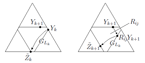
Figure 6. Illustration of Lemma 4.1 (i) (left), (ii) (middle) and (iii) (right)
Proof.

To prove (i), we assume 𝐱{\bf x} is not of the form i​jm−1ij^{m-1}. Then on the event {Yk=𝐱}\{Y_{k}={\bf x}\}, we have Tk+1=Tk+1T_{k+1}=T_{k}+1, and so Yk+1=ZTk+1Y_{k+1}=Z_{T_{k}+1}. It follows from the strong Markov property that

ℙϑ​{Yk+1=𝐲|Yk=𝐱}=ℙϑ​{ZTk+1=𝐲|ZTk=𝐱}=1deg⁡(𝐱).{\mathbb{P}}_{\vartheta}\{Y_{k+1}={\bf y}|Y_{k}={\bf x}\}={\mathbb{P}}_{\vartheta}\{Z_{{T_{k}}+1}={\bf y}|Z_{T_{k}}={\bf x}\}=\frac{1}{\mathrm{deg}({\bf x})}.

For (ii), let B={Ri​j(𝐱a):j=0,…,d}B=\{R_{ij}({\bf x}a):j=0,...,d\}, τ2=inf{n≥0:|Zn|=2}\tau_{2}=\inf\{n\geq 0:|Z_{n}|=2\} and q𝐳=ℙ𝐳{Zτ2∈B}q_{{\bf z}}={\mathbb{P}}_{{\bf z}}\{Z_{\tau_{2}}\in B\}. Then ℙϑ​{Yk+1∈B|Yk=𝐱}=q𝐱{\mathbb{P}}_{\vartheta}\{Y_{k+1}\in B|Y_{k}={\bf x}\}=q_{{\bf x}}. By standard first-step calculations, we have

qϑ\displaystyle q_{\vartheta} =\displaystyle= ∑j=0d1d+1​qj,\displaystyle\sum_{j=0}^{d}\frac{1}{d+1}q_{j},
qj\displaystyle q_{j} =\displaystyle= 12​d+2​1+12​d+2​qϑ+∑l=0,l≠jd12​d+2​ql,j=0,…,d.\displaystyle\frac{1}{2d+2}1+\frac{1}{2d+2}q_{\vartheta}+\sum_{l=0,l\neq j}^{d}\frac{1}{2d+2}q_{l},\ \ \ j=0,...,d.

Note that deg⁡(j)=1+d+(d+1)=2​d+2{\mathrm{deg}}(j)=1+d+(d+1)=2d+2. Solving the equations, we get qj=qϑ=1d+1q_{j}=q_{\vartheta}=\frac{1}{d+1} for all jj.

The proof of (iii) is similar to that of (ii). ∎

To define the reflected process {Z~k}\{\tilde{Z}_{k}\}, we need to keep track of the parity changes of {Yk}\{Y_{k}\}. We define a strictly increasing sequence {Sp}p≥0\{S_{p}\}_{p\geq 0} of {𝒢m}\{{\mathcal{G}}_{m}\}-stopping times by S0=0S_{0}=0,

Sp+1=inf{m>Sp:[Ym]≠[YSp]},p≥0.S_{p+1}=\inf\{m>S_{p}:[Y_{m}]\neq[Y_{S_{p}}]\},\ \ \ p\geq 0.

Also define a random sequence {Gp}\{G_{p}\} in 𝒜d{\mathcal{A}}_{d} by G0=R0,[Y0]G_{0}=R_{0,[Y_{0}]},

Gp+1=Gp∘R[YSp],[YSp+1],p≥0.G_{p+1}=G_{p}\circ R_{[Y_{S_{p}}],[Y_{S_{p+1}}]},\ \ \ p\geq 0.

Hence

Gp=R0,[Y0]∘R[Y0],[YS1]∘⋯∘R[YSp−1],[YSp]G_{p}=R_{0,[Y_{0}]}\circ R_{[Y_{0}],[Y_{S_{1}}]}\circ\cdots\circ R_{[Y_{S_{p-1}}],[Y_{S_{p}}]}

is a random product of reflections induced by {Yk}\{Y_{k}\}. We leave GpG_{p} undefined if Sp=∞S_{p}=\infty. Finally, for k≥0k\geq 0, we define

Z~k=Gp​Yk, if ​Sp≤k<Sp+1.\tilde{Z}_{k}=G_{p}Y_{k},\ \ \ \text{ if }S_{p}\leq k<S_{p+1}.

By induction, one can check that Z~k∈0​X\tilde{Z}_{k}\in 0X for all k≥0k\geq 0. For each kk, let LkL_{k} be the unique random integer such that Lk​(ω)=pL_{k}(\omega)=p if Sp​(ω)≤k<Sp+1​(ω)S_{p}(\omega)\leq k<S_{p+1}(\omega). Then Z~k=GLk​Yk\tilde{Z}_{k}=G_{L_{k}}Y_{k} for all kk. See Figure 7 for an illustration.

Refer to caption
Figure 7. Suppose that [Yk]=i[Y_{k}]=i and [Yk+1]=j[Y_{k+1}]=j, where i≠ji\neq j. Then Z~k+1\tilde{Z}_{k+1} is defined as Z~k+1=(GLk∘Ri​j)​Yk\tilde{Z}_{k+1}=(G_{L_{k}}\circ R_{ij})Y_{k}.
Example 4.2.

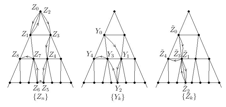
Consider the case d=1d=1. We compute YkY_{k}, GLkG_{L_{k}} and Z~k\tilde{Z}_{k} for the following sample path of {Zn}n=08\{Z_{n}\}_{n=0}^{8}:

nn 00 11 22 33 44 55 66 77 88
ZnZ_{n} ϑ\vartheta 00 ϑ\vartheta 11 1010 100100 001001 0101 0000
kk 00 11 22 33 44
YkY_{k} 00 1010 100100 0101 0000
LkL_{k} 00 11 11 22 22
GLkG_{L_{k}} i​did R01R_{01} R01R_{01} i​did i​did
Z~k\tilde{Z}_{k} 00 0101 011011 0101 0000
Refer to caption
Figure 8. Illustration of the processes {Zn}\{Z_{n}\}, {Yk}\{Y_{k}\} and {Z~k}\{\tilde{Z}_{k}\}

The main result of this section is the following.

Proposition 4.3.

Under ℙϑ{\mathbb{P}}_{\vartheta}, {Z~k}k≥0\{\tilde{Z}_{k}\}_{k\geq 0} is a simple random walk on 0​X0X with ℙϑ{Z~0=0}=1{\mathbb{P}}_{\vartheta}\{\tilde{Z}_{0}=0\}=1.

Proof.

We first check that ℙϑ{Z~0=0}=1{\mathbb{P}}_{\vartheta}\{\tilde{Z}_{0}=0\}=1. Under ℙϑ{\mathbb{P}}_{\vartheta}, we have almost surely that T0=1T_{0}=1. Hence Y0=Z1Y_{0}=Z_{1} and GL0=G0=R0,[Y0]G_{L_{0}}=G_{0}=R_{0,[Y_{0}]}. It follows that Z~0=R0,[Y0]​Y0=0\tilde{Z}_{0}=R_{0,[Y_{0}]}Y_{0}=0 almost surely.

Next we prove by induction on NN that

ℙϑ{Z~k=𝐳k,0≤k≤N}=∏k=0N−11deg0​(𝐳k){\mathbb{P}}_{\vartheta}\{\tilde{Z}_{k}={\bf z}_{k},0\leq k\leq N\}=\prod_{k=0}^{N-1}\frac{1}{\mathrm{deg}_{0}({\bf z}_{k})}

for any path {𝐳k}k=0N\{{\bf z}_{k}\}_{k=0}^{N} in 0​X0X such that 𝐳0=0{\bf z}_{0}=0. Here deg0\mathrm{deg}_{0} denotes the degree in the subgraph 0​X0X, and, by convention, the product is 11 when N=0N=0. This establishes that {Z~k}\{\tilde{Z}_{k}\} is a simple random walk on 0​X0X.

The case N=0N=0 is trivial. Assume the claim for paths of length NN and consider the probability

ℙϑ{Z~k=𝐳k,0≤k≤N+1}.{\mathbb{P}}_{\vartheta}\{\tilde{Z}_{k}={\bf z}_{k},0\leq k\leq N+1\}.

The idea is to condition on the value of GLNG_{L_{N}}. By iterated expectation,

ℙϑ{Z~k=𝐳k,0≤k≤N+1}\displaystyle{\mathbb{P}}_{\vartheta}\{\tilde{Z}_{k}={\bf z}_{k},0\leq k\leq N+1\} (4.1)
=\displaystyle= 𝔼ϑ[𝔼ϑ(∏k=0N+1𝟏{Z~k=𝐳k}|𝒢N)]\displaystyle{\mathbb{E}}_{\vartheta}\left[{\mathbb{E}}_{\vartheta}\left(\prod_{k=0}^{N+1}{\bf 1}\{\tilde{Z}_{k}={\bf z}_{k}\}|{\mathcal{G}}_{N}\right)\right]
=\displaystyle= ∑g∈𝒜d𝔼ϑ[∏k=0N𝟏{Z~k=𝐳k}𝟏{GLN=g}𝔼ϑ(𝟏{GLN+1YN+1=𝐳N+1}|𝒢N)].\displaystyle\sum_{g\in{\mathcal{A}}_{d}}{\mathbb{E}}_{\vartheta}\left[\prod_{k=0}^{N}{\bf 1}\{\tilde{Z}_{k}={\bf z}_{k}\}{\bf 1}\{G_{L_{N}}=g\}{\mathbb{E}}_{\vartheta}\left({\bf 1}\{G_{L_{N+1}}Y_{N+1}={\bf z}_{N+1}\}|{\mathcal{G}}_{N}\right)\right].

In the last equality we use the fact that {GLk}\{G_{L_{k}}\} and {Z~k}\{\tilde{Z}_{k}\} are adapted to {𝒢k}\{{\mathcal{G}}_{k}\}.

Now we distinguish three cases and use Lemma 4.1.
(i) 𝐳N{\bf z}_{N} is not of the form 0​jm−10j^{m-1} where j≠0j\neq 0 and m≥1m\geq 1. Then on the event {Z~N=𝐳N,GLN=g}\{\tilde{Z}_{N}={\bf z}_{N},G_{L_{N}}=g\} we have YN=g−1​Z~NY_{N}=g^{-1}\tilde{Z}_{N} and GLN+1=GLN=gG_{L_{N+1}}=G_{L_{N}}=g. It follows that on the event {Z~N=𝐳N,GLN=g}\{\tilde{Z}_{N}={\bf z}_{N},G_{L_{N}}=g\} we have

𝔼ϑ[𝟏{GLN+1YN+1=𝐳N+1}|𝒢K]\displaystyle{\mathbb{E}}_{\vartheta}[{\bf 1}\{G_{L_{N+1}}Y_{N+1}={\bf z}_{N+1}\}|{\mathcal{G}}_{K}] (4.2)
=\displaystyle= ℙϑ​{g​YN+1=𝐳N+1|𝒢N}\displaystyle{\mathbb{P}}_{\vartheta}\{gY_{N+1}={\bf z}_{N+1}|{\mathcal{G}}_{N}\}
=\displaystyle= ℙϑ​{g​YN+1=𝐳N+1|YN}\displaystyle{\mathbb{P}}_{\vartheta}\{gY_{N+1}={\bf z}_{N+1}|Y_{N}\}
=\displaystyle= ℙϑ​{YN+1=g−1​𝐳N+1|YN=g−1​𝐳N}\displaystyle{\mathbb{P}}_{\vartheta}\{Y_{N+1}=g^{-1}{\bf z}_{N+1}|Y_{N}=g^{-1}{\bf z}_{N}\}
=\displaystyle= 1deg⁡(g−1​𝐳N)\displaystyle\frac{1}{\mathrm{deg}(g^{-1}{\bf z}_{N})} (4.3)
=\displaystyle= 1deg⁡(𝐳N).\displaystyle\frac{1}{\mathrm{deg}({\bf z}_{N})}.

In the above, equality in (4.2) is the simple Markov property of {Yk}\{Y_{k}\}, and (4.3) follows from Lemma 4.1(i). Note that deg⁡(g−1​𝐳N)=deg⁡(𝐳N)=deg0​(𝐳N)\mathrm{deg}(g^{-1}{\bf z}_{N})=\mathrm{deg}({\bf z}_{N})=\mathrm{deg}_{0}({\bf z}_{N}). Putting this into (4.1) and continuing the calculation, we get from the induction hypothesis that

ℙϑ{Z~k=𝐳k,1≤k≤N+1}\displaystyle{\mathbb{P}}_{\vartheta}\{\tilde{Z}_{k}={\bf z}_{k},1\leq k\leq N+1\}
=\displaystyle= ∑g∈𝒜d𝔼[∏k=0N𝟏{Z~k=𝐳k}𝟏{GLN=g}1deg0​(𝐳N)]\displaystyle\sum_{g\in{\mathcal{A}}_{d}}{\mathbb{E}}\left[\prod_{k=0}^{N}{\bf 1}\{\tilde{Z}_{k}={\bf z}_{k}\}{\bf 1}\{G_{L_{N}}=g\}\frac{1}{\mathrm{deg}_{0}({\bf z}_{N})}\right]
=\displaystyle= 1deg0​(𝐳N)𝔼[∏k=0N1{Z~k=𝐳k}]\displaystyle\frac{1}{\mathrm{deg}_{0}({\bf z}_{N})}{\mathbb{E}}\left[\prod_{k=0}^{N}1\{\tilde{Z}_{k}={\bf z}_{k}\}\right]
=\displaystyle= ∏k=0N1deg0​(𝐳k).\displaystyle\prod_{k=0}^{N}\frac{1}{\mathrm{deg}_{0}({\bf z}_{k})}.

The remaining cases are similar.
(ii) 𝐳N=0{\bf z}_{N}=0. On the event {Z~N=𝐳N,GLN=g}\{\tilde{Z}_{N}={\bf z}_{N},G_{L_{N}}=g\}, we have

𝔼ϑ[𝟏{Z~N+1=𝐳N+1}|𝒢N]\displaystyle{\mathbb{E}}_{\vartheta}[{\bf 1}\{\tilde{Z}_{N+1}={\bf z}_{N+1}\}|{\mathcal{G}}_{N}]
=\displaystyle= ℙϑ​{YN+1∈⋃j=0d{(g∘R[g−1​𝐳N],j)−1​𝐳N+1}|YN=g−1​𝐳N},\displaystyle{\mathbb{P}}_{\vartheta}\{Y_{N+1}\in\bigcup_{j=0}^{d}\{(g\circ R_{[g^{-1}{\bf z}_{N}],j})^{-1}{\bf z}_{N+1}\}|Y_{N}=g^{-1}{\bf z}_{N}\},

and by Lemma 4.1(ii) this equals 1d+1=1deg0​(0)\frac{1}{d+1}=\frac{1}{{\mathrm{deg}}_{0}(0)}.
(iii) 𝐳N=0​jm−1{\bf z}_{N}=0j^{m-1} where j≠0j\neq 0 and m≥2m\geq 2. If GLN=gG_{L_{N}}=g, then g−1​𝐳Ng^{-1}{\bf z}_{N} has a unique horizontal neighbor whose parity (say ii) is different from that of g−1​𝐳Ng^{-1}{\bf z}_{N}. Then, on the event {Z~N=𝐳N,GLN=g}\{\tilde{Z}_{N}={\bf z}_{N},G_{L_{N}}=g\}, we have

𝔼ϑ[𝟏{Z~N+1=𝐳N+1}|𝒢N]\displaystyle{\mathbb{E}}_{\vartheta}[{\bf 1}\{\tilde{Z}_{N+1}={\bf z}_{N+1}\}|{\mathcal{G}}_{N}]
=\displaystyle= ℙϑ{YN+1∈{g−1𝐳N+1,(g∘Ri,[g−1​𝐳N])−1𝐳N+1|YN=g−1𝐳N},\displaystyle{\mathbb{P}}_{\vartheta}\{Y_{N+1}\in\{g^{-1}{\bf z}_{N+1},(g\circ R_{i,[g^{-1}{\bf z}_{N}]})^{-1}{\bf z}_{N+1}|Y_{N}=g^{-1}{\bf z}_{N}\},

which equals 1deg⁡(𝐳N)−1=1deg0​(𝐳N)\frac{1}{{\mathrm{deg}}({\bf z}_{N})-1}=\frac{1}{{\mathrm{deg}_{0}}({\bf z}_{N})} by Lemma 4.1(iii). ∎

5. Self-similar identity and hitting distribution

First we relate the hitting distribution of {Z~k}\{\tilde{Z}_{k}\} with that of {Zn}\{Z_{n}\}. Since 0​X0X is isomorphic to XX, we may regard 0​X0X as the augmented rooted tree of the IFS {F0​i}i=0d\{F_{0i}\}_{i=0}^{d} with self-similar set K0K_{0}. It follows that {Z~k}\{\tilde{Z}_{k}\}, which is a simple random walk on 0​X0X, converges almost surely to a point on K0K_{0}. Thus we get:

Lemma 5.1.

Under ℙϑ{\mathbb{P}}_{\vartheta}, Z~k\tilde{Z}_{k} converges almost surely to a point Z~∞\tilde{Z}_{\infty} on K0⊂KK_{0}\subset K. For any Borel set BB in K0K_{0}, we have

ℙϑ{Z~∞∈B}=ℙϑ{Z∞∈F0−1(B)}=νϑ(F0−1(B)).{\mathbb{P}}_{\vartheta}\{\tilde{Z}_{\infty}\in B\}={\mathbb{P}}_{\vartheta}\{Z_{\infty}\in F_{0}^{-1}(B)\}=\nu_{\vartheta}(F_{0}^{-1}(B)).

Next we consider the relation between Z∞Z_{\infty} and Z~∞\tilde{Z}_{\infty}. Recall that pi​jp_{ij} is the midpoint of the vertices pip_{i} and pjp_{j}.

Lemma 5.2.

There exists G∞∈𝒜dG_{\infty}\in{\mathcal{A}}_{d}, depending on ω\omega, such that Z~∞=G∞​Z∞\tilde{Z}_{\infty}=G_{\infty}Z_{\infty}.

Proof.

Fix ω\omega such that Z∞​(ω)Z_{\infty}(\omega) exists and we will suppress ω\omega in what follows. Since YkY_{k} is a subsequence of ZnZ_{n}, we have

Z∞=Y∞:=limk→∞Yk.Z_{\infty}=Y_{\infty}:=\lim_{k\rightarrow\infty}Y_{k}.

First suppose that Z~∞≠p0​i\tilde{Z}_{\infty}\neq p_{0i} for all i≠0i\neq 0. We claim that there exists NN such that ρ⁡(Yk)=ρ⁡(YN)\rho(Y_{k})=\rho(Y_{N}) for all k≥Nk\geq N. That is, the parity stays constant for kk large enough. To see this, note that the parity changes only when Z~k=0​il\tilde{Z}_{k}=0i^{l} for some ii and ll. Now since Z~∞≠p0​i\tilde{Z}_{\infty}\neq p_{0i}, there is some ϵ>0\epsilon>0 and L∈ℕL\in{\mathbb{N}} such that when kk is large, dist⁡(ι⁡(Z~k),K0​iL)≥ϵ{\mathrm{dist}}(\iota(\tilde{Z}_{k}),K_{0i^{L}})\geq\epsilon for all ii. It follows that Z~k≠0​il\tilde{Z}_{k}\neq 0i^{l}, where l≥Ll\geq L, when kk is large. Hence GLk=GLN=:G∞G_{L_{k}}=G_{L_{N}}=:G_{\infty} for all k≥Nk\geq N and

Z~k=G∞​Yk,k≥N.\tilde{Z}_{k}=G_{\infty}Y_{k},\ \ \ k\geq N.

Letting k→∞k\rightarrow\infty, we get Z~∞=G∞​Y∞=G∞​Z∞\tilde{Z}_{\infty}=G_{\infty}Y_{\infty}=G_{\infty}Z_{\infty}.

Next suppose that Z~∞=p0​i\tilde{Z}_{\infty}=p_{0i} for some ii. Since every g∈𝒜dg\in{\mathcal{A}}_{d} must map p0​ip_{0i} to some other midpoint, by convergence of {Yk}\{Y_{k}\} we see that for large kk, [Yk][Y_{k}] takes at most two values, say jj and ll. Hence, there exists G∈𝒜dG\in{\mathcal{A}}_{d} such that for each sufficiently large kk, GLkG_{L_{k}} is either GG or G∘Rj​lG\circ R_{jl}. We may take G∞G_{\infty} to be any one which appears infinitely often. ∎

Let 𝒜d′={g∈𝒜d:g​K0=K0}{\mathcal{A}}^{\prime}_{d}=\{g\in{\mathcal{A}}_{d}:gK_{0}=K_{0}\} be the subgroup of 𝒜d{\mathcal{A}}_{d} that fixes the cell K0K_{0}. It corresponds to the subgroup of 𝒮d+1{\mathcal{S}}_{d+1} that fixes the symbol 00 and hence is isomorphic to 𝒮d{\mathcal{S}}_{d}. The next lemma, which is purely geometric, is straightforward to prove.

Lemma 5.3.

Suppose B⊂K0B\subset K_{0} is Borel and is invariant under 𝒜d′{\mathcal{A}}^{\prime}_{d}, i.e., g​B=BgB=B for all g∈𝒜d′g\in{\mathcal{A}}^{\prime}_{d}. Then ⋃i=0dR0​i​B\bigcup_{i=0}^{d}R_{0i}B is invariant under 𝒜d{\mathcal{A}}_{d}, i.e.,

g⁡(⋃i=0dR0​i​B)=⋃i=0dR0​i​B,g∈𝒜d.g(\bigcup_{i=0}^{d}R_{0i}B)=\bigcup_{i=0}^{d}R_{0i}B,\ \ \ g\in{\mathcal{A}}_{d}.

Moreover, (⋃i=0dR0​i​B)∩K0=B\left(\bigcup_{i=0}^{d}R_{0i}B\right)\cap K_{0}=B.

The reason of using 𝒜d′{\mathcal{A}}^{\prime}_{d}-invariant sets is that for fixed Z∞Z_{\infty}, Z~∞=G∞​Z∞\tilde{Z}_{\infty}=G_{\infty}Z_{\infty} may take one of several values depending on the sequence of reflections made.

Lemma 5.4.

Suppose B⊂K0B\subset K_{0} is Borel and is 𝒜d′{\mathcal{A}}^{\prime}_{d}-invariant. Then

{Z~∞∈B}={Z∞∈⋃i=0dR0​iB}.\{\tilde{Z}_{\infty}\in B\}=\{Z_{\infty}\in\bigcup_{i=0}^{d}R_{0i}B\}.
Proof.

By Lemma 5.2, Z~∞=G∞​Z∞\tilde{Z}_{\infty}=G_{\infty}Z_{\infty} for some (random) G∞∈𝒜dG_{\infty}\in{\mathcal{A}}_{d}. If Z~∞∈B\tilde{Z}_{\infty}\in B, then

Z∞=G∞−1​Z~∞∈G∞−1​B⊂⋃i=0dR0​i​BZ_{\infty}=G_{\infty}^{-1}\tilde{Z}_{\infty}\in G_{\infty}^{-1}B\subset\bigcup_{i=0}^{d}R_{0i}B

by Lemma 5.3. On the other hand, suppose Z∞∈⋃i=0dR0​i​BZ_{\infty}\in\bigcup_{i=0}^{d}R_{0i}B for some ii and let G∞G_{\infty} be as above. By Lemma 5.3 again, we have

Z~∞=G∞​Z∞∈(G∞​⋃i=0dR0​i​B)∩K0=B.\tilde{Z}_{\infty}=G_{\infty}Z_{\infty}\in\left(G_{\infty}\bigcup_{i=0}^{d}R_{0i}B\right)\cap K_{0}=B.

∎

By Lemmas 5.1 and 5.4, we immediately obtain the following crucial result.

Theorem 5.5.

(Self-similar identity) Suppose B⊂K0B\subset K_{0} is Borel and is 𝒜d′{\mathcal{A}}^{\prime}_{d}-invariant, i.e., g​B=BgB=B for all g∈𝒜d′g\in{\mathcal{A}}^{\prime}_{d}. Then

νϑ​(S0−1​B)=νϑ​(⋃i=0dR0​i​B).\nu_{\vartheta}(S_{0}^{-1}B)=\nu_{\vartheta}(\bigcup_{i=0}^{d}R_{0i}B).
Refer to caption
Figure 9. The two sets have the same probability under νϑ\nu_{\vartheta}.

We are now ready to prove the main theorem.

Proof of Theorem 1.1. Let μ\mu be the normalized α\alpha-dimensional Hausdorff measure on KK, where α=dimHK\alpha=\dim_{H}K. We will show that μ\mu is the unique Borel probability measure on KK that satisfies the identities in Theorems 3.5 and 5.5. Since νϑ\nu_{\vartheta} has been shown to satisfy these identifies, this implies that νϑ=μ\nu_{\vartheta}=\mu.

Let λ\lambda be any Borel probability measure on KK satisfying the identities. We will complete the proof assuming the claim that λ\lambda has no atoms on the dyadic points, i.e., λ⁡(p𝐱)=0\lambda(p_{{\bf x}})=0 for all 𝐱∈X∖{ϑ}{\bf x}\in X\setminus\{\vartheta\}. This allows us to use additivity for sets that intersect only at dyadic points.

It suffices to show that λ⁡(K𝐱)=1(d+1)|𝐱|\lambda(K_{{\bf x}})=\frac{1}{(d+1)^{|{\bf x}|}} for all 𝐱∈X{\bf x}\in X. We proceed by induction on |𝐱||{\bf x}|, the length of 𝐱{\bf x}. By definition of λ\lambda, we have λ⁡(K)=1\lambda(K)=1. For the first level, we have

1=λ⁡(K)=λ⁡(⋃i=0dKi)=λ⁡(K0)+∑i=1dλ⁡(R0​i​K0)=(d+1)​λ​(K0),1=\lambda(K)=\lambda(\bigcup_{i=0}^{d}K_{i})=\lambda(K_{0})+\sum_{i=1}^{d}\lambda(R_{0i}K_{0})=(d+1)\lambda(K_{0}),

where in the last equality we used group invariance and the fact that R0​i​K0=KiR_{0i}K_{0}=K_{i}. Hence λ⁡(Ki)=1/(d+1)\lambda(K_{i})=1/(d+1) for all ii.

Now suppose that λ⁡(K𝐱)=1(d+1)|𝐱|\lambda(K_{{\bf x}})=\frac{1}{(d+1)^{|{\bf x}|}} for all 𝐱{\bf x} with |𝐱|=m|{\bf x}|=m. Applying the self-similar identity, we have

1(d+1)m=λ⁡(K0m)=λ⁡(⋃i=0dKim+1)=(d+1)​λ​(K0m+1).\frac{1}{(d+1)^{m}}=\lambda(K_{0^{m}})=\lambda(\bigcup_{i=0}^{d}K_{i^{m+1}})=(d+1)\lambda(K_{0^{m+1}}).

Hence λ⁡(K0m+1)=1(d+1)m\lambda(K_{0^{m+1}})=\frac{1}{(d+1)^{m}}. Next, fix any 𝐱\bf x with |𝐱|=m|{\bf x}|=m and 𝐱≠0m{\bf x}\neq 0^{m}. Consider the set

⋃g∈𝒜d′g​K0​𝐱⊂K0.\bigcup_{g\in{\mathcal{A}}^{\prime}_{d}}gK_{0{\bf x}}\subset K_{0}.

Observe that the sets in the union intersect only at dyadic points and is invariant under 𝒜d′{\mathcal{A}}^{\prime}_{d}. By the self-similar identity, we have

λ⁡(⋃g∈𝒜d′g​K𝐱)=λ⁡(S0−1​⋃g∈𝒜d′g​K0​𝐱)=λ⁡(⋃i=0d⋃g∈𝒜d′g​K0​𝐱).\lambda(\bigcup_{g\in{\mathcal{A}}^{\prime}_{d}}gK_{\bf x})=\lambda(S_{0}^{-1}\bigcup_{g\in{\mathcal{A}}^{\prime}_{d}}gK_{0{\bf x}})=\lambda(\bigcup_{i=0}^{d}\bigcup_{g\in{\mathcal{A}}^{\prime}_{d}}gK_{0{\bf x}}).

Using group invariance and the fact that #⁡(𝒜d′)=d!\#({\mathcal{A}}^{\prime}_{d})=d!, we get

d!(d+1)m=(d+1)​d!​λ​(K0​𝐱).\frac{d!}{(d+1)^{m}}=(d+1)d!\lambda(K_{0{\bf x}}).

It follows that λ⁡(K0​𝐱)=1(d+1)m+1\lambda(K_{0{\bf x}})=\frac{1}{(d+1)^{m+1}} for all |𝐱|=m|{\bf x}|=m, and applying R0​iR_{0i}, i≠0i\neq 0, this implies that λ⁡(K𝐲)=1(d+1)m+1\lambda(K_{{\bf y}})=\frac{1}{(d+1)^{m+1}} for all |𝐲|=m+1|{\bf y}|=m+1. This completes the induction argument.

It remains to verify the claim that λ⁡(p𝐱)=0\lambda(p_{{\bf x}})=0 for all 𝐱{\bf x}. The proof is to show by induction on the level of 𝐱{\bf x} that all p𝐱p_{\bf x} have equal probability. The method is the same as the above induction and we leave the argument to the reader. And since the set of dyadic points is infinite, this implies that the probability is 00.

□\Box

6. Remarks and open questions

There are many more things that can be said in this model. Using the reflection principle and induction on NN, we can show the following:

Proposition 6.1.

For N≥0N\geq 0, let τN=inf{n≥0:|Zn|=N}\tau_{N}=\inf\{n\geq 0:|Z_{n}|=N\}. Then under ℙϑ{\mathbb{P}}_{\vartheta}, the distribution of ZτNZ_{\tau_{N}} is uniform on {0,…,d}N\{0,...,d\}^{N}.

The idea of the proof is to reformulate the group invariance and self-similar identities in terms of ZτNZ_{\tau_{N}} and Z~τN\tilde{Z}_{\tau_{N}}. For example, the group invariance identity will take the form

ℙϑ{ZτN∈B}=ℙϑ{ZτN∈gB},B⊂{0,…,d}N.{\mathbb{P}}_{\vartheta}\{Z_{\tau_{N}}\in B\}={\mathbb{P}}_{\vartheta}\{Z_{\tau_{N}}\in gB\},\ \ \ B\subset\{0,...,d\}^{N}.

Since Z~k\tilde{Z}_{k} is the simple random walk on 0​X0X starting at 00, the distribution of Z~τN\tilde{Z}_{\tau_{N}} can be expressed by that of ZτN−1Z_{\tau_{N-1}}. This allows us to use the induction hypothesis (and for small NN the proposition follows by direct calculations). Together with a limiting argument, this gives an alternative approach to Theorem 1.1.

We have only shown that νϑ=μ\nu_{\vartheta}=\mu. How about ν𝐱\nu_{{\bf x}} for 𝐱≠ϑ{\bf x}\neq\vartheta? As remarked in the beginning of Section 5, the reflection principle can be formulated for any starting point. For other starting points, the same method can be used to show the following:

Proposition 6.2.

Let 𝐱=0​𝐲∈0​X{\bf x}=0{\bf y}\in 0X, where 𝐲∈X{\bf y}\in X. Define σ​𝐱=𝐲\sigma{\bf x}={\bf y}. Then νσ​𝐱​(S0−1​B)=ν𝐱​(⋃i=0dR0​i​B)\nu_{\sigma{\bf x}}(S_{0}^{-1}B)=\nu_{{\bf x}}(\bigcup_{i=0}^{d}R_{0i}B) for all B⊂K0B\subset K_{0} which is invariant under 𝒜d′{\mathcal{A}}^{\prime}_{d}.

Q1. Can the above be used to derive estimates of ν𝐱\nu_{{\bf x}}?

Our method does not require any estimate of the Martin kernel, and this is both an advantage and a disadvantage. Even for the simplest case d=1d=1, we have not been able to derive good estimates of the Martin kernels.

Q2. When d=1d=1, can we prove directly (without using the hyperbolic boundary as in [WL]) that the Martin boundary is homeomorphic to [0,1][0,1]?

It is natural to consider generalization of the reflection principle to other highly symmetric augmented rooted trees. As we have seen, the crucial objects needed is that each i​XiX is isomorphic to XX, and there is a ‘local’ reflection Ri​j∈Aut⁡(i​X∪j​X)R_{ij}\in\mathrm{Aut}(iX\cup jX) (and a corresponding map on KK) whenever i≠ji\neq j. Indeed, there are many cases where our method is applicable. An example is the pentagon fractal.

Refer to caption
Figure 10. The pentagon fractal with a reflection R01R_{01}.

Here the symmetry group is the dihedral group D5D_{5}. Another example is Lindstrøm’s snowflake (see [Ku]), where the symmetry group is the dihedral group D6D_{6}. For both cases the hitting distribution starting from the root ϑ\vartheta is uniform. The arguments are the same and we leave the details to the reader. So far we have not been able to generalize this to an axiomatic framework such as the class of nested fractals (see [Ku]).

Q3. Can the results of this paper be generalized to all nested fractals?

We may think about the simple random walks on Sierpinski graphs as a special case of the framework in [WL]. In that general setting, very little is known about the hitting distributions. As is mentioned in the introduction, these measures serve as the reference measures of the induced Dirichlet forms in [WL], and understanding them is of value to analyze the associated jump processes.

Q4. For the simple (or a strictly reversible, see [WL]) random walk on the augmented rooted tree of a self-similar set satisfying OSC, are the hitting distributions absolutely continuous with respect to the Hausdorff (or a self-similar) measure?

Acknowledgements
The author would like to thank Professor Ka-Sing Lau for his guidance and support during the preparation of this paper.

References

  • [A] A. Ancona, Positive harmonic functions and hyperbolicity, J. Kral, Editor, Potential Theory: Surveys and Problems, Lecture Notes in Mathematics 1344, Springer-Verlag, Berlin/Heidelberg (1988), pp. 1–23.
  • [DS1] M. Denker and H. Sato, Sierpinski gasket as a Martin boundary I: Martin kernels, Potential Anal. 14 (2001), no. 3, 211-232.
  • [DS2] M. Denker and H. Sato, Sierpinski gasket as a Martin boundary II: The intrinsic metric, Publ. Res. Inst. Math. Sci. 35 (1999), no. 5, 769-794.a
  • [DS3] M. Denker and H. Sato, Reflections on harmonic analysis of the Sierpinski gasket, Math. Nachr. 241 (2002), 32-55.
  • [G] M. Gromov, Hyperbolic groups, Essays in group theory, Math. Sci. Res. Inst. Publ., 8, Springer, New York, 1987, 75-263.
  • [JLW] H. Ju, K.-S. Lau and X.-Y. Wang, Post-critically finite fractal and Martin boundary, Amer. Math. Soc. (2010) (to appear).
  • [K] V.A. Kaimanovich, Random walks on Sierpinski graphs: hyperbolicity and stochastic homogenization, Fractals in Graz 2001, 145-183, Trends Math., Birkhäuser, Basel, 2003.
  • [Ki] J. Kigami, Dirichlet forms and associated heat kernels on the Cantor set induced by random walks on trees, Adv. in Math. 225 (2010), Issue 5, 2674-2730.
  • [Ku] S. Kusuoka, Lecture on diffusion processes on nested fractals, Statistical mechanics and fractals, 39-98 Lecture Notes in Mathematics, 1567. Springer-Verlag, Berlin, 1993.
  • [LN] K.-S. Lau and S.-M. Ngai, Martin boundary and exit space on the Sierpinski gasket, preprint.
  • [LW1] K.-S. Lau and X.-Y. Wang, Self-similar sets as hyperbolic boundaries, Indiana Univ. Math. J. 58 (2009), no. 4, 1777-1795.
  • [LW2] K.-S. Lau and X.-Y. Wang, Self-similar sets, hyperbolic boundaries and Martin boundaries, preprint.
  • [N] J. Norris, Markov chains, Cambridge University Press, 1998.
  • [P] E. Pearse, Self-similar fractals as boundaries of network, preprint available at http://arxiv.org/abs/1104.1650
  • [WL] T.-K. L. Wong and K.-S. Lau, Random walks and induced Dirichlet forms on self-similar sets, submitted.
  • [Wo] W. Woess, Random walks on infinite graphs and groups, Cambridge Tracts in Mathematics 138, Combridge University Press, Cambridge 2000.