Efficient Generation of Random Bits from Finite State Markov Chains
Abstract
The problem of random number generation from an uncorrelated random source (of unknown probability distribution) dates back to von Neumann’s 1951 work. Elias (1972) generalized von Neumann’s scheme and showed how to achieve optimal efficiency in unbiased random bits generation. Hence, a natural question is what if the sources are correlated? Both Elias and Samuelson proposed methods for generating unbiased random bits in the case of correlated sources (of unknown probability distribution), specifically, they considered finite Markov chains. However, their proposed methods are not efficient or have implementation difficulties. Blum (1986) devised an algorithm for efficiently generating random bits from degree-2 finite Markov chains in expected linear time, however, his beautiful method is still far from optimality on information-efficiency. In this paper, we generalize Blum’s algorithm to arbitrary degree finite Markov chains and combine it with Elias’s method for efficient generation of unbiased bits. As a result, we provide the first known algorithm that generates unbiased random bits from an arbitrary finite Markov chain, operates in expected linear time and achieves the information-theoretic upper bound on efficiency.
Index Terms:
Random sequence, Random bits generation, Markov chain.I Introduction
The problem of random number generation dates back to von Neumann [8] who considered the problem of simulating an unbiased coin by using a biased coin with unknown probability. He observed that when one focuses on a pair of coin tosses, the events and have the same probability ( is for ‘head’ and is for ‘tail’); hence, produces the output symbol and produces the output symbol . The other two possible events, namely, and , are ignored, namely, they do not produce any output symbols. More efficient algorithms for generating random bits from a biased coin were proposed by Hoeffding and Simons [6], Elias [3], Stout and Warren [16] and Peres [11]. Elias [3] was the first to devise an optimal procedure in terms of the information efficiency, namely, the expected number of unbiased random bits generated per coin toss is asymptotically equal to the entropy of the biased coin. In addition, Knuth and Yao [7] presented a simple procedure for generating sequences with arbitrary probability distributions from an unbiased coin (the probability of and is ). Han and Hoshi [4] generalized this approach and considered the case where the given coin has an arbitrary known bias.
In this paper, we study the problem of generating random bits from an arbitrary and unknown finite Markov chain (the transition matrix is unknown). The input to our problem is a sequence of symbols that represent a random trajectory through the states of the Markov chain - given this input sequence our algorithm generates an independent unbiased binary sequence called the output sequence. This problem was first studied by Samuelson [13]. His approach was to focus on a single state (ignoring the other states) treat the transitions out of this state as the input process, hence, reducing the problem of correlated sources to the problem of a single ‘independent’ random source; obviously, this method is not efficient. Elias [3] suggested to utilize the sequences related to all states: Producing an ‘independent’ output sequence from the transitions out of every state and then pasting (concatenating) the collection of output sequences to generate a long output sequence. However, neither Samuelson nor Elias proved that their methods work for arbitrary Markov chains, namely, they did not prove that the transitions out of each state are independent. In fact, Blum [1] probably realized it, as he mentioned that: (i) “Elias’s algorithm is excellent, but certain difficulties arise in trying to use it (or the original von Neumann scheme) to generate bits in expected linear time from a Markov chain”, and (ii) “Elias has suggested a way to use all the symbols produced by a MC (Markov Chain). His algorithm approaches the maximum possible efficiency for a one-state MC. For a multi-state MC, his algorithm produces arbitrarily long finite sequences. He does not, however, show how to paste these finite sequences together to produce infinitely long independent unbiased sequences.” Blum [1] derived a beautiful algorithm to generate random bits from a degree-2 Markov chain in expected linear time by utilizing the von Neumann scheme for generating random bits from biased coin flips. While his approach can be extended to arbitrary out-degrees (the general Markov chain model used in this paper), the information-efficiency is still far from being optimal due to the low information-efficiency of the von Neumann scheme.
In this paper, we generalize Blum’s algorithm to arbitrary degree finite Markov chains and combine it with existing methods for efficient generation of unbiased bits from biased coins, such as Elias’s method. As a result, we provide the first known algorithm that generates unbiased random bits from arbitrary finite Markov chains, operates in expected linear time and achieves the information-theoretic upper bound on efficiency. Specifically, we propose an algorithm (that we call Algorithm ), that is a simple modification of Elias’s suggestion to generate random bits, it operates on finite sequences and its efficiency can asymptotically reach the information-theoretic upper bound for long input sequences. In addition, we propose a second algorithm, called Algorithm , that is a combination of Blum’s and Elias’s algorithms, it generates infinitely long sequences of random bits in expected linear time. One of our key ideas for generating random bits is that we explore equal-probability sequences of the same length. Hence, a natural question is: Can we improve the efficiency by utilizing as many as possible equal-probability sequences? We provide a positive answer to this question and describe Algorithm , that is the first known polynomial-time and optimal algorithm (it is optimal in terms of information-efficiency for an arbitrary input length) for random bits generation from finite Markov chains.
In this paper, we use the following notations:
The remainder of this paper is organized as follows. Section II reviews existing schemes for generating random bits from arbitrarily biased coins. Section III discusses the challenge in generating random bits from arbitrary finite Markov chains and presents our main lemma - this lemma characterizes the exit sequences of Markov chains. Algorithm is presented and analyzed in Section IV, it is related to Elias’s ideas for generating random bits from Markov chains. Algorithm is presented in Section V, it is a generalization of Blum’s algorithm. An optimal algorithm, called Algorithm , is described in Section VI. Finally, Section VII provides numerical evaluations of our algorithms.
II Generating Random Bits for Biased Coins
Consider a sequence of length generated by a biased n-face coin
such that the probability to get is , and . While we are given a sequence the probabilities that are unknown, the question is: How can we efficiently generate an independent and unbiased sequence of ’s and ’s from ? The efficiency (information-efficiency) of a generation algorithm is defined as the ratio between the expected length of the output sequence and the length of the input sequence, namely, the expected number of random bits generated per input symbol. In this section we describe three existing solutions for the problem of random bits generation from biased coins.
II-A The von Neumann Scheme
In 1951, von Neumann [8] considered this question for biased coins and described a simple procedure for generating an independent unbiased binary sequence from the input sequence . In his original procedure, the coin is binary, however, it can be simply generalized for the case of an -face coin: For an input sequence, we can divide it into pairs and use the following mapping for each pair
where denotes the empty sequence. As a result, by concatenating the outputs of all the pairs, we can get a binary sequence which is independent and unbiased. The von Neumann scheme is computationally (very) efficient, however, its information-efficiency is far from being optimal. For example, when the input sequence is binary, the probability for a pair of input bits to generate an output bit (not a ) is , hence the efficiency is , which is at and less elsewhere.
II-B The Elias Scheme
In 1972, Elias [3] proposed an optimal (in terms of efficiency) algorithm as a generalization of the von Neumann scheme; for the sake of completeness we describe it here.
Elias’s method is based on the following idea: The possible input sequences of length can be partitioned into classes such that all the sequences in the same class have the same number of ’s with . Note that for every class, the members of the class have the same probability to be generated. For example, let and , we can divide the possible input sequences into 5 classes:
Now, our goal is to assign a string of bits (the output) to each possible input sequence, such that any two output sequences and with the same length (say ), have the same probability to be generated, namely for some . The idea is that for any given class we partition the members of the class to groups of sizes that are a power of 2, for a group with members (for some ) we assign binary strings of length . Note that when the class size is odd we have to exclude one member of this class. We now demonstrate the idea by continuing the example above.
Note that in the example above, we cannot assign any bits to the sequence in , so if the input sequence is , the output sequence should be (denotes the empty sequence). There are sequences in and we assign the binary strings as follows:
Similarly, for , there are sequences that can be divided into a group of and a group of :
In general, for a class with members that were not assigned yet, assign possible output binary sequences of length to distinct unassigned members, where . Repeat the procedure above for the rest of the members that were not assigned. Note that when a class has an odd number of members, there will be one and only one member assigned to .
Given an input sequence of length , using the method above, the output sequence can be written as a function of , denoted by , called the Elias function. In [12], Ryabko and Matchikina showed that the Elias function of an input sequence of length (that is generated by a biased coin with two faces) is computable in time. We can prove that their conclusion is valid in the general case of a coin with faces with .
II-C The Peres Scheme
In 1992, Peres [11] demonstrated that iterating the original von Neumann scheme on the discarded information can asymptotically achieve optimal efficiency. Let’s define the function related to the von Neumann scheme as . Then the iterated procedures with are defined inductively. Given input sequence , let denote all the indices for which , then is defined as
Note that on the righthand side of the equation above, the first term corresponds to the random bits generated with the von Neumann scheme, the second and third terms relate to the symmetric information discarded by the von Neumann scheme.
Finally, we can define for sequences of odd length by
Surprisingly, this simple iterative procedure achieves the optimal efficiency asymptotically. The computational complexity and memory requirements of this scheme are substantially smaller than those of the Elias scheme. However, a drawback of this scheme is that its generalization to the case of an -face coin with is not obvious.
II-D Properties of the Schemes
Let’s denote as a scheme that generates independent unbiased sequences from any biased coins (with unknown probabilities). Such can be the von Neumann scheme, the Elias scheme, the Peres scheme or any other scheme. Let be a sequence generated from an arbitrary biased coin, with length , then a property of is that for any and with , we have
Namely, two output sequences of equal length have equal probability.
That leads to the following property for . It says that given the number of ’s for all with , the number of such sequences to yield a binary sequence equals to that of sequences to yield if and have the same length. It further implies that given the condition of knowing the number of ’s for all with , the output sequence of is still independent and unbiased. This property is due to the linear independence of probability functions of the sequences with different numbers of the ’s.
Lemma 1.
Let be a subset in such that it includes all the sequences with the same number of ’s for all with , namely, . Let denote the set . Then for any and with , we have .
Proof.
In , the number of ’s in each sequence is for all , then we can get that
where
Since , we have
The set of polynomials is linearly independent in the vector space of functions on , so we can conclude that . ∎
| Input sequence | Probability | ||
|---|---|---|---|
| 1 | |||
III Some Properties of Markov Chains
Our goal is to efficiently generate random bits from a Markov chain with unknown transition probabilities. The paradigm we study is that a Markov chain generates the sequence of states that it is visiting and this sequence of states is the input sequence to our algorithm for generating random bits. Specifically, we express an input sequence as with , where indicate the states of a Markov chain.
One idea is that for a given Markov chain, we can treat each state, say , as a coin and consider the ‘next states’ (the states the chain has transitioned to after being at state ) as the results of a coin toss. Namely, we can generate a collection of sequences , called exit sequences, where is the sequence of states following in , namely,
For example, assume that the input sequence is
If we consider the states following we get as the set of states in boldface:
Hence, the exit sequences are:
Lemma 2 (Uniqueness).
An input sequence can be uniquely determined by and .
Proof.
Given and , according to the work of Blum in [1], can uniquely be constructed in the following way: Initially, set the starting state as . Inductively, if , then set as the first element in and remove the first element of . Finally, we can uniquely generate the sequence . ∎
Lemma 3 (Equal-probability).
Two input sequences and with have the same probability to be generated if for all .
Proof.
Note that the probability to generate is
and the probability to generate is
By permutating the terms in the expression above, it is not hard to get that if and for all . Basically, the exit sequences describe the edges that are used in the trajectory in the Markov chain. The edges in the trajectories that correspond to and are identical, hence . ∎
In [13], Samuelson considered a two-state Markov chain, and he pointed out that it may generate unbiased random bits by applying the von Neumann scheme to the exit sequence of state . Later, in [3], in order to increase the efficiency, Elias has suggested a scheme that uses all the symbols produced by a Markov chain. His main idea was to create the final output sequence by concatenating the output sequences that correspond to . However, neither Samuelson nor Elias proved that their methods produce random output sequences that are independent and unbiased, in fact, their proposed methods are not correct for some cases. To demonstrate it we consider: (1) as the final output. (2) as the final output. For example, consider the two-state Markov chain in which and , as shown in Fig. 1.

Assume that an input sequence of length is generated from this Markov chain and the starting state is , then the probabilities of the possible input sequences and their corresponding output sequences are given in Table I. In the table we can see that the probabilities to produce or are different for some and in both methods, presented in columns 3 and 4, respectively.
The problem of generating random bits from an arbitrary Markov chain is challenging, as Blum said in [1]: “Elias’s algorithm is excellent, but certain difficulties arise in trying to use it (or the original von Neumann scheme) to generate random bits in expected linear time from a Markov chain”. It seems that the exit sequence of a state is independent since each exit of the state will not affect the other exits. However, this is not always true when the length of the input sequence is given, say . Let’s still consider the example of a two-state Markov chain in Fig. 1. Assume the starting state of this Markov chain is , if , then with non-zero probability we have
whose length is . But it is impossible to have
of length . That means is not an independent sequence. The main reason is that although each exit of a state will not affect the other exits, it will affect the length of the exit sequence. In fact, is an independent sequence if the length of is given, instead of giving the length of .
In this paper, we consider this problem from another perspective. According to Lemma 3, we know that permutating the exit sequences does not change the probability of a sequence, however, the permuted sequence has to correspond to a trajectory in the Markov chain. The reason for this contingency is that in some cases the permuted sequence does not correspond to a trajectory: Consider the following example,
and
If we permutate the last exit sequence to , we cannot get a new sequence such that its starting state is and its exit sequences are
This can be verified by attempting to construct the sequence using Blum’s method (which is given in the proof of Lemma 2). Notice that if we permutate the first exit sequence into , we can find such a new sequence, which is
This observation motivated us to study the characterization of exit sequences that are feasible in Markov chains (or finite state machines).
Definition 1 (Feasibility).
Given a Markov chain, a starting state and a collection of sequences , we say that is feasible if and only if there exists a sequence that corresponds to a trajectory in the Markov chain such that and .
Based on the definition of feasibility, we present the main technical lemma of the paper. Repeating the notation from the beginning of the paper, we say that a sequence is a tail-fixed permutation of , denoted as , if and only if (1) is a permutation of , and (2) and have the same last element, namely, .
Lemma 4 (Main Lemma: Feasibility and equivalence of exit sequences).
Given a starting state and two collections of sequences and such that (tail-fixed permutation) for all . Then is feasible if and only if is feasible.
The proof of this main lemma will be given in the Appendix. According to the main lemma, we have the following equivalent statement.
Lemma 5 (Feasible permutations of exit sequences).
Given an input sequence with that produced from a Markov chain. Assume that is an aribitrary collection of exit sequences that corresponds to the exit sequences of as follows:
- 1.
is a permutation () of , for .
- 2.
is a tail-fixed permutation () of , for .
Then there exists a feasible sequence such that and . For this , we have .
One might reason that Lemma 5 is stronger than the main lemma (Lemma 4). However, we will show that these two lemmas are equivalent. It is obvious that if the statement in Lemma 5 is true, then the main lemma is also true. Now we show that if the main lemma is true then the statement in Lemma 5 is also true.
Proof.
Given , let’s add one more symbol to the end of ( is different from all the states in ), then we can get a new sequence , whose exit sequences are
According to the main lemma, we know that there exists another sequence such that its exit sequences are
and . Definitely, the last symbol of this sequence is , i.e., . As a result, we have .
Now, by removing the last element from , we can get a new sequence such that its exit sequences are
and . We also have .
This completes the proof. ∎
We demonstrate the result above by considering the example at the beginning of this section. Let
with and its exit sequences is given by
After permutating all the exit sequences (for , we keep the last element of the sequence fixed), we get a new group of exit sequences
Based on these new exit sequences, we can generate a new input sequence
This accords with the statements above.
IV Algorithm A : Modification of Elias’s Suggestion
In the section above, we see that Elias suggested to paste the outputs of different exit sequences together, as the final output, but the simple direct concatenation cannot always work. By modifying the method of pasting these outputs, we get Algorithm to generate unbiased random bits from any Markov chains.
-
Algorithm A
-
Input: A sequence produced by a Markov chain, where .
-
Output: A sequence of s and s.
-
Main Function:
Suppose .for doif thenOutput .elseOutputend ifend for -
Comment: (1) can be any scheme that generates random bits from biased coins. For example, we can use the Elias function. (2) When , we can also output for simplicity, but the efficiency may be reduced a little.
The only difference between Algorithm and direct concatenation is that: Algorithm ignores the last symbols of some exit sequences. Let’s go back to the example of a two-state Markov chain with and in Fig. 1, which demonstrates that direct concatenation does not always work well. Here, we still assume that an input sequence with length is generated from this Markov chain and the starting state is , then the probability of each possible input sequence and its corresponding output sequence (based on Algorithm ) are given by:
| Input sequence | Probability | Output sequence |
|---|---|---|
We can see that when the input sequence length , a bit and a bit have the same probability to be generated and no longer sequences are generated. In this case, the output sequence is independent and unbiased.
In order to prove that all the sequences generated by Algorithm are independent and unbiased, we need to show that for any sequences and of the same length, they have the same probability to be generated.
Theorem 6 (Algorithm A).
Let the sequence generated by a Markov chain be used as input to Algorithm , then the output of Algorithm is an independent unbiased sequence.
Proof.
Let’s first divide all the possible sequences in into groups, and use to denote the set of the groups. Two sequences and are in the same group if and only if
- 1.
and for some .
- 2.
If , .
- 3.
If , .
We will show that for each group , the number of sequences to generate equals to that of sequences to generate if and have the same length, i.e., if , where is the set of sequences of length that yield .
Now, given a group , if let’s define as the set of all the permutations of for , and if let’s define as the set of all the permutations of for . According to Lemma 1, we know that for any , there are the same number of members in which generate and . So we can use to denote the number of members in which generate a certain binary sequence with length (e.g. ).
According to the definitions above, let be non-negative integers, then we have
where each combination is a partition of the length of .
Similarly, we also have
which tells us that if .
Note that all the sequences in the same group have the same probability to be generated. So when , the probability to generate is
which implies that output sequence is independent and unbiased. ∎
Theorem 7 (Efficiency).
Let be a sequence of length generated by a Markov chain, which is used as input to Algorithm . Let in Algorithm be Elias’s function. Suppose the length of its output sequence is , then the limiting efficiency as realizes the upper bound .
Proof.
Here, the upper bound is provided by Elias [3]. We can use the same argument in Elias’s paper [3] to prove this theorem.
Let denote the next state of . Obviously, is a random variable for , whose entropy is denoted as . Let denote the stationary distribution of the Markov chain, then we have
When , there exists an which , such that with probability , for all . Using Algorithm A, with probability , the length of the output sequence is bounded below by
where is the efficiency of the when the input is or . According to Theorem 2 in Elias’s paper [3], we know that as , . So with probability , the length of the output sequence is below bounded by
Then we have
At the same time, is upper bounded by . So we can get
which completes the proof. ∎
Given an input sequence, it is efficient to generate independent unbiased sequences using Algorithm . However, it has some limitations: (1) The complete input sequence has to be stored. (2) For a long input sequence it is computationally intensive as it depends on the input length. (3) The method works for finite-length sequences and does not lend itself to stream processing. In order to address these limitations we propose two variants of Algorithm .
In the first variant of Algorithm , instead of applying directly to for (or for ), we first split into several segments with lengths then apply to all of the segments separately. It can be proved that this variant of Algorithm A can generate independent unbiased sequences from an arbitrary Markov chain, as long as do not depend on the order of elements in each exit sequence. For example, we can split into two segments of lengths and , we can also split it into three segments of lengths … Generally, the shorter each segment is, the faster we can obtain the final output. But at the same time, we may have to sacrifice a little information efficiency.
The second variant of Algorithm is based on the following idea: for a given sequence from a Markov chain, we can split it into some shorter sequences such that they are independent of each other, therefore we can apply Algorithm to all of the sequences and then concatenate their output sequences together as the final one. In order to do this, given a sequence , we can use as a special state to it. For example, in practice, we can set a constant , if there exists a minimal integer such that and , then we can split into two sequences and (note that both of the sequences have the element ). For the second sequence , we can repeat the some procedure … Iteratively, we can split a sequence into several sequences such that they are independent of each other. These sequences, with the exception of the last one, start and end with , and their lengths are usually slightly longer than .
V Algorithm B : Generalization of Blum’s Algorithm
In [1], Blum proposed a beautiful algorithm to generate an independent unbiased sequence of ’s and ’s from any Markov chain by extending von Neumann scheme. His algorithm can deal with infinitely long sequences and use only constant space and expected linear time. The only drawback of his algorithm is that its efficiency is still far from the information-theoretic upper bound, due to the limitation (compared to the Elias algorithm) of the von Neumann scheme. In this section, we generalize Blum’s algorithm by replacing von Neumann scheme with Elias’s. As a result, we get Algorithm : It maintains some good properties of Blum’s algorithm and its efficiency approaches the information-theoretic upper bound.
-
Algorithm B
-
Input: A sequence (or a stream) produced by a Markov chain, where .
-
Parameter: positive integer functions (window size) with for .
-
Output: A sequence (or a stream) of ’s and ’s.
-
Main Function:
(empty) for all .for all .the index of current state, namely, .while next input symbol is ( null) do(Add to ).if thenOutput ...end if.end while
In the algorithm above, we apply function on to generate random bits if and only if the window for is completely filled and the Markov chain is currently at state .
For example, we set for all and the input sequence is
After reading the last second () symbol , we have
In this case, so the window for is full, but we don’t apply to because the current state of the Markov chain is , not .
By reading the last () symbol , we get
Since the current state of the Markov chain is and , we produce and reset as .
In the example above, treating as input to Algorithm , we can get the output sequence is . The algorithm does not output until the Markov chain reaches state again. Timing is crucial!
Note that Blum’s algorithm is a special case of Algorithm by setting the window size functions for all and . Namely, Algorithm is a generalization of Blum’s algorithm, the key is that when we increase the windows sizes, we can apply more efficient schemes (compared to the von Neumann scheme) for . Assume a sequence of symbols with have been read by the algorithm above, we want to show that for any , the output sequence is always independent and unbiased. Unfortunately, Blum’s proof for the case of cannot be applied to our proposed scheme.
For all with , we can write
where with are the segments used to generate outputs. For all , we have
and
See Fig. 2 for simple illustration.

Theorem 8 (Algorithm ).
Let the sequence generated by a Markov chain be used as input to Algorithm , then Algorithm generates an independent unbiased sequence of bits in expected linear time.
Proof.
In the following proof, we use the same idea as in the proof for Algorithm .
Let’s first divide all the possible input sequences in into groups, and use to denote the group set. Two sequences and are in the same group if and only if
- 1.
and .
- 2.
For all with ,
where and are the segments used to generate outputs.
- 3.
For all , .
- 4.
For all , .
We will show that in each group , the number of sequences to generate equals to that of sequences to generate if , i.e., for , where is the set of sequences of length that yield .
Now, given a group , let’s define as the set of all the permutations of for . According to Lemma 1, we know that for different , there are the same number of members in which generate . So we can use to denote the number of members in which generate a certain binary sequence with length .
Let be non-negative integers such that their sum is , we want to prove that
The proof is by induction. Let . First, the conclusion holds for . Assume the conclusion holds for , we want to prove that the conclusion also holds for .
Given an , assume is the last segment that generates an output. According to our main lemma (Lemma 4), we know that for any sequence in , is always the last segment that generates an output. Now, let’s fix and assume generates the last bits of . We want to know how many sequences in have as their last segments that generate outputs? In order to get the answer, we concatenate with as the new . As a result, we have segments to generate the first bits of . Based on our assumption, the number of such sequences will be
where are non-negative integers. For a different , there are choices for . Therefore, can be obtained by multiplying by the number above and summing them up over . Namely, we can get the conclusion above.
According to this conclusion, we know that if , then . Using the same argument as in Theorem 6 we complete the proof of the theorem. ∎
Normally, the window size functions for can be any positive integer functions. Here, we fix these window size functions as a constant, namely, . By increasing the value of , we can increase the efficiency of the scheme, but at the same time it may cost more storage space and need more waiting time. It is helpful to analyze the relationship between scheme efficiency and window size .
Theorem 9 (Efficiency).
Let be a sequence of length generated by a Markov chain with transition matrix , which is used as input to Algorithm with constant window size . Then as the length of the sequence goes to infinity, the limiting efficiency of Algorithm is
where is the stationary distribution of this Markov chain, and is the efficiency of when the input sequence of length is generated by a -face coin with distribution .
Proof.
When , there exists an which , such that with probability , for all .
The efficiency of Algorithm can be written as , which satisfies
With probability , we have
So when , we have that
This completes the proof. ∎
Let’s define , where is the standard binary expansion of . Assume is the Elias function, then
Based on this formula, we can numerically study the relationship between the limiting efficiency and the window size (see Section VII). In fact, when the window size becomes large, the limiting efficiency () approaches the information-theoretic upper bound.
VI Algorithm C : An Optimal Algorithm
Both Algorithm and Algorithm are asymptotically optimal, but when the length of the input sequence is finite they may not be optimal. In this section, we try to construct an optimal algorithm, called Algorithm C, such that its information-efficiency is maximized when the length of the input sequence is finite. Before presenting this algorithm, following the idea of Pae and Loui[10], we first discuss the equivalent condition for a function to generate random bits from an arbitrary Markov chain, and then present the sufficient condition for to be optimal.
Lemma 10 (Equivalent condition).
Let be an non-negative integer matrix with . We define as
where is the number of in . A function can generate random bits from an arbitrary Markov chain, if and only if for any and two binary sequences and with ,
where is the set of sequences of length that yield .
Proof.
If can generate random bits from an arbitrary Markov chain, then for any two binary sequences and of the same length. Here, we can write
where and is the probability to generate a sequence with starting state and with exit sequences specified by if such input sequence exists. Similarly,
As a result,
Since can be any value in , for all we have
According to the linear independence of in the vector space of functions on , we can conclude that for all if .
Inversely, if for all with the same length, for all , then and have the same probability to be generated. Therefore, can generate random bits from an arbitrary Markov chain. ∎
Let’s define , where is the standard binary expansion of , then we have the sufficient condition for an optimal function .
Lemma 11 (Sufficient condition for an optimal function).
Let be a function that generates random bits from an arbitrary Markov chain with unknown transition probabilities. If for any and any non-negative integer matrix with , the following equation is satisfied,
then generates independent unbiased random bits with optimal information efficiency. Note that is the length of and is the size of .
Proof.
Let denote an arbitrary function that is able to generate random bits from any Markov chain. According to Lemma 2.9 in [10], we know that
Then the average output length of is
So is the optimal one. This completes the proof. ∎
Here, we construct the following algorithm (Algorithm ) which satisfies all the conditions in Lemma 10 and Lemma 11. As a result, it can generate unbiased random bits from an arbitrary Markov chain with optimal information efficiency.
-
Algorithm C
-
Input: A sequence produced by a Markov chain, where .
-
Output: A sequence of s and s.
-
Main Function:
1) Get the matrix with2) Define as
then compute .3) Compute the rank of in with respect to a given order.4) According to and , determine the output sequence. Let be the standard binary expansion of with and assume the starting value of is . If , the output is the digit binary representation of . If , the output is the digit binary representation of . -
Comment: The fast calculations of and will be given in the rest of this section.
In Algorithm , when we use Elias’s function as , the limiting efficiency (as ) realizes the bound . Algorithm is optimal, so it has the same or higher efficiency. Therefore, the limiting efficiency of Algorithm as also realizes the bound .
In Algorithm , for an input sequence with , we can rank it with respect to the lexicographic order of and . Here, we define
which is the vector of the last symbols of for . And is the complement of in , namely,
For example, when the input sequence is
Its exit sequences is
Then for this input sequence , we have that
Based on the lexicographic order defined above, both and can be obtained using a brute-force search. However, this approach in not computationally efficient. Here, we describe an efficient algorithm for computing and , such that Algorithm is computable in time. This method is inspired by the algorithm for computing the Elias function that is described in [12].
Lemma 12.
in Algorithm is computable in time.
Proof.
The idea to compute in Algorithm is that we can divide into different classes, denoted by for different such that
where is the number of ’s in for all . is the vector of the last symbols of defined above. As a result, we have . Although it is not easy to calculate directly, but it is much easier to compute for a given .
For a given , we need first determine whether is empty or not. In order to do this, we quickly construct a collection of exit sequences by moving the first in to the end for all . According to the main lemma, we know that is empty if and only if does not include for some or is not feasible.
If is not empty, then is feasible. In this case, based on the main lemma, we have
where the first term, denoted by , is computable in time [2]. Further more, we can get that
is also computable in time. ∎
Lemma 13.
in Algorithm is computable in time.
Proof.
Based on some calculations in the lemma above, we can try to obtain when is ranked with respect to the lexicographic order of and . Let denote the rank of in , then we have that
where is based on the lexicographic order. In the formula, can be efficiently obtained by computing
where is defined in the last lemma. So far, we only need to compute , with respect to the lexicography order of . can be written as a group of sequences such that for all
There are symbols in . Let be the number of sequences such that the first symbols of are the same with that of and the symbol of is smaller than that of , then we can get that
Assume the symbol in is the symbol in . Then we can get that
where is the subsequence of from the symbol to the end; is the number of permutations for .
Let’s define the values
where is the index of the first symbol of , i.e., . Then can be written as
Suppose that is an integer. Otherwise, we can add trivial terms to the formula above to make an integer. In order to quickly calculate , the following calculations are performed:
Then applying the method in [12], we have that
which is computable in time. As a result, for a fixed , is computable in time. ∎
Based on the discussion above, we know that Algorithm is computable in time.
VII Numerical Results
In this section, we describe numerical results related to the implementations of Algorithm , Algorithm , and Algorithm . We use the Elias function for .
In the first experiment, we use the following randomly generated a transition matrix for a Markov chain with three states.
Consider a sequence of length that is generated by the Markov chain defined above and assume that is the first state of this sequence. Namely, there are possible input sequences. For each possible input sequence, we can compute its generating probability and the corresponding output sequences using our three algorithms. Table II presents the results of calculating the probabilities of all possible output sequences for the three algorithms. Note that the results show that indeed the outputs of the algorithms are independent unbiased sequences. Also, Algorithm has the highest information efficiency (it is optimal), and Algorithm has a higher information efficiency than Algorithm (with window size 4).
| Output | Probability | Probability | Probability |
|---|---|---|---|
| Algorithm | Algorithm | Algorithm | |
| with | |||
| 0.0224191 | 0.1094849 | 0.0208336 | |
| 0 | 0.0260692 | 0.0215901 | 0.0200917 |
| 1 | 0.0260692 | 0.0215901 | 0.0200917 |
| 00 | 0.0298179 | 0.1011625 | 0.0206147 |
| 10 | 0.0298179 | 0.1011625 | 0.0206147 |
| 01 | 0.0298179 | 0.1011625 | 0.0206147 |
| 11 | 0.0298179 | 0.1011625 | 0.0206147 |
| 000 | 0.0244406 | 0.0242258 | 0.0171941 |
| 100 | 0.0244406 | 0.0242258 | 0.0171941 |
| … | |||
| 011111 | 0.0018831 | 1.39E-5 | 0.0029596 |
| 111111 | 0.0018831 | 1.39E-5 | 0.0029596 |
| 0000000 | 1.305E-4 | 6.056E-4 | |
| 1000000 | 1.305E-4 | 6.056E-4 | |
| 0111111 | 1.305E-4 | 6.056E-4 | |
| 1111111 | 1.305E-4 | 6.056E-4 | |
| 00000000 | 1.44E-5 | ||
| 10000000 | 1.44E-5 | ||
| 01111111 | 1.44E-5 | ||
| 11111111 | 1.44E-5 | ||
| Expected Length | 3.829 | 2.494 | 4.355 |

In the second calculation, we want to test the influence of window size (assume for ) on the efficiency of Algorithm . Since the efficiency depends on the transition matrix of the Markov chain we decided to evaluate of the efficiency related to the uniform transition matrix, namely all the entries are , where is the number of states. We assume that is infinitely large. In this case, the stationary distribution of the Markov chain is . Fig. 3 shows that when (Blum’s Algorithm), the limiting efficiencies for are , respectively. When , their corresponding efficiencies are . So if the input sequence is long enough, by changing from to , the efficiency can increase for , for and for . When is small, we can increase the efficiency of Algorithm significantly by increasing the window size . When becomes larger, the efficiency of Algorithm will converge to the information-theoretical upper bound, namely, . Note that is not a good value for the window size in the algorithm. That is because the Elias function is not very efficient when the length of the input sequence is . Let’s consider a biased coin with two states . If the input sequence is or , the Elias function will generate nothing. For all other cases, it has only chance to generate one bit and chance to generate nothing. As a result, the efficiency is even worse than the efficiency when the length of the input sequence equals to .
VIII Concluding Remarks
We considered the classical problem of generating independent unbiased bits from an arbitrary Markov chain with unknown transition probabilities. Our main contribution is the first known algorithm that has expected linear time complexity and achieves the information-theoretic upper bound on efficiency.
Our work is related to a number of interesting results in both computer science and information theory. In computer science, the attention has focused on extracting randomness from a general weak source (introduced by Zuckerman [17]). Hence, the concept of an extractor was introduced - it converts weak random sequences to ‘random-looking’ sequences, using an additional small number of truly random bits. During the past two decades, extractors and their applications have been studied extensively, see [9][14] for surveys on the topic. While our algorithms generate truly random bits (given a prefect Markov chain as a source) the goal of extractors is to generate ‘random-looking’ sequences which are asymptotically close to random bits.
In information theory, it was discovered that optimal source codes can be used as universal random bits generators from arbitrary stationary ergodic random sources [15][5]. When the input sequence is generated from a stationary ergodic process and it is long enough one can obtain an output sequence that behaves like truly random bits in the sense of normalized divergence. However, in some cases, the definition of normalized divergence is not strong enough. For example, suppose is a sequence of unbiased random bits in the sense of normalized divergence, and is with a concatenated at the beginning. If the sequence is long enough the sequence is a sequence of unbiased random bits in the sense of normalized divergence. However the sequence might not be useful in applications that are sensitive to the randomness of the first bit.
In this appendix, we prove the main lemma.
Lemma 4 (Main Lemma: Feasibility and equivalence of exit sequences). Given a starting state and two collections of sequences and such that (tail-fixed permutation) for all . Then is feasible if and only if is feasible.
In the rest of the appendix we will prove the main lemma. To illustrate the claim in the lemma, we express and by a directed graph that has labels on the vertices and edges, we call this graph a sequence graph. For example, when and , we have the directed graph in Fig. 4.
Let denote the vertex set, then
and the edge set is
For each edge , the label of this edge is . For the edge , the label is . Namely, the label set of the outgoing edges of each state is .

Given the labeling of the directed graph as defined above, we say that it contains a complete walk if there is a path in the graph that visits all the edges, without visiting an edge twice, in the following way: (1) Start from . (2) At each vertex, we choose an unvisited edge with the minimal label to follow. Obviously, the labeling corresponding to is a complete walk if and only if is feasible. In this case, for short, we also say that is a complete walk. Before continuing to prove the main lemma, we first give Lemma 14 and Lemma 15.
Lemma 14.
Assume with is a a complete walk, which ends at state . Then with is also a complete walk ending at , if (permutation).
Proof.
and correspond to different labelings on the same directed graph , denoted by and . Since is a complete walk, it can travel all the edges in one by one, denoted as
where and . We call as the indexes of the edges.
Based on , let’s have a walk on starting from until there is no unvisited outgoing edges to select. In this walk, assume the following edges have been visited:
where are distinct indexes chosen from and . In order to prove that is a complete walk, we need to show that (1) and (2) .
First, let’s prove that . In , let denote the number of outgoing edges of and let denote the number of incoming edges of , then we have that
Based on these relations, we know that once we have a walk starting from in , this walk will finally end at state . That is because we can always get out of due to if .
Now, we prove that . This can be proved by contradiction. Assume , then we define
where corresponds to the visited edges based on and corresponds to the unvisited edges based on . Let , then is the unvisited edge with the minimal index. Let , then is an outgoing edge of . Here , because all the outgoing edges of have been visited. Assume the number of visited incoming edges of is and the number of visited outgoing edges of is , then
see Fig. 5 as an example.
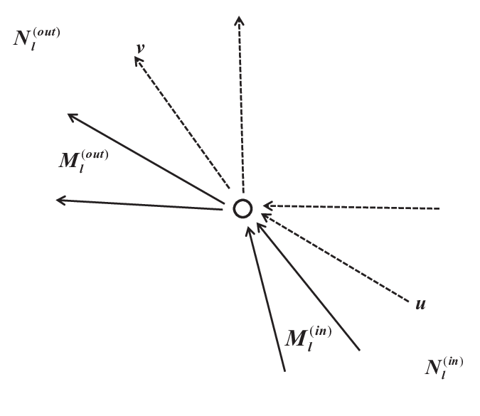
Note that the labels of the outgoing edges of are the same for and , since . Therefore, based on , before visiting edge , there must be outgoing edges of have been visited. As a result, based on , there must be incoming edges of have been visited before visiting . Among all these incoming edges, there exists at least one edge such that , since only incoming edges of have been visited based on .
According to our assumption, both and is the minimal one, so . On the other hand, we know that is visited before based on , so . Here, the contradiction happens. Therefore, .
This completes the proof. ∎
Here, let’s give an example of the lemma above. We know that, when , is feasible. The labeling on a directed graph corresponding to is given in Fig. 4, which is a complete walk starting at state and ending at state . The path of the walk is
By permutating the labels of the outgoing edges of , we can have the graph as shown in Fig. 6. The new labeling on is also a complete walk ending at state , and its path is

Based on Lemma 14, we have the following result
Lemma 15.
Given a starting state and two collections of sequences and such that (tail-fixed permutation). Then and have the same feasibility.
Proof.
We prove that if is feasible, then is also feasible. If is feasible, there exists a sequence such that and . Suppose its last element is .
When , according to Lemma 14, we know that is feasible.
When , we assume that . Let’s consider the subsequence of . Then and the last element of is . According to Lemma 14, we can get that: there exists a sequence with and such that
since .
Let , i.e., concatenating to the end of , we can generate a sequence such that its exit sequence of state is
and its exit sequence of state with is .
So if is feasible, then is also feasible. Similarly, if is feasible, then is feasible. As a result, and have the same feasibility. ∎
According to the lemma above, we know that and have the same feasibility, and have the same feasibility, …, and have the same feasibility, so the statement in the main lemma is true.
References
- [1] M. Blum, “Independent unbiased coin flips from a correlated biased source: a finite state Markov chain”, Combinatorica, vol. 6, pp. 97-108, 1986.
- [2] P. B. Borwein, “On the complexity of calculating factorials”, Journal of Algorithms, vol. 6, pp. 376-380, 1985.
- [3] P. Elias, “The efficient construction of an unbiased random sequence”, Ann. Math. Statist., vol. 43, pp. 865-870, 1972.
- [4] T. S. Han and M. Hoshi, “Interval algorithm for random number generation”, IEEE Trans. on Information Theory, vol. 43, No. 2, pp. 599-611, 1997.
- [5] T. S. Han, “Folklore in source coding: information-spectrum approach”, IEEE Trans. on Information Theory, vol. 51, no. 2, pp. 747-753, 2005.
- [6] W. Hoeffding and G. Simon, “Unbiased coin tossing with a biased coin”, Ann. Math. Statist., vol. 41, pp. 341-352, 1970.
- [7] D. Knuth and A. Yao, “The complexity of nonuniform random number generation”, Algorithms and Complexity: New Directions and Recent Results, pp. 357-428, 1976.
- [8] J. von Neumann, “Various techniques used in connection with random digits”, Appl. Math. Ser., Notes by G.E. Forstyle, Nat. Bur. Stand., vol. 12, pp. 36-38, 1951.
- [9] N. Nisan, “Extracting randomness: how and why. A survey”, in Proc. Eleventh Annual IEEE conference on Computational Complexity, pp. 44-58, 1996.
- [10] S. Pae and M. C. Loui, “Optimal random number generation from a biased coin”, in Proc. Sixteenth Annu. ACM-SIAM Symp. Discrete Algorithms, pp. 1079-1088, 2005.
- [11] Y. Peres, “Iterating von Neumann’s procedure for extracting random bits”, Ann. Statist., vol. 20, pp. 590-597, 1992.
- [12] B. Y. Ryabko and E. Matchikina, “Fast and efficient construction of an unbiased random sequence”, IEEE Trans. on Information Theory, vol. 46, pp. 1090-1093, 2000.
- [13] P. A. Samuelson, “Constructing an unbiased random sequence”, J. Amer. Statist. Assoc, pp. 1526-1527, 1968.
- [14] R. Shaltiel, “Recent developments in explicit constructions of extractors”, BULLETIN-European Association For Theoretical Computer Science, vol 77, pp. 67-95, 2002.
- [15] K. Visweswariah, S. R. Kulkarni and S. Verdú, “Source codes as random number generators”, IEEE Trans. on Information Theory, vol. 44, no. 2, pp. 462-471, 1998.
- [16] Q. Stout and B. Warren, “Tree algorithms for unbiased coin tosssing with a biased coin”, Ann. Probab., vol. 12, pp. 212-222, 1984.
- [17] D. Zuckerman, “General weak random sources”, in Proc. of the 31st IEEE Symposium on Foundations of Computer Science, pp. 534-543, 1990.