On light propagation in Swiss-Cheese cosmologies

Hereafter, we assume $\Lambda=0$. The large scale evolution is given by the LT solution with

$$\begin{array}[]{ccc}E(r)=0\;,&\epsilon(t,r)=\frac{1}{6\pi t^{2}}\;,&t_{B}(r)=0\;.\end{array}$$

(8)

This choice corresponds to the EdS model. At some time $t_{init}$ we match inhomogeneities. They are modelled by the following LT solution. We make the same choice as in [2007PhRvD..76l3004M] and take

$$\epsilon(t_{init},r)=A\exp^{-\frac{1}{2}\left(\frac{r-r_{M}}{\varsigma}\right)^{2}}+\delta\;.$$

(9)

Moreover, we assume $R(t_{init},r)=r$ and this together with (6) determines $t_{B}(r)$. The formula for $E(r)$ follows from the assumption that at $t=t_{init}$ the speed of the angular expansion of the inhomogeneous regions equals to the speed of the expansion of the homogeneous part. It is

$$E(r)=\frac{2}{9}\left(\frac{r}{t_{init}}\right)^{2}-\frac{M}{r}\;.$$

(10)

Summarizing, the profile of inhomogeneities at time $t_{init}$ is given in comoving coordinates by the size of the inhomogeneity $r_{b}$, the position of a peak of the density $r_{M}$, it’s amplitude $A$ and the width $\varsigma$, and finally, the parameter $\delta$ that controls the density at the centres of the inhomogeneous regions. The parameters $A$, $r_{M}$ are not arbitrary, but they are chosen to satisfy the matching conditions (7). We have found

$$A=\left(\frac{1}{6\pi t_{init}^{2}}-\delta\right)\exp^{\frac{1}{2}\left(\frac{r_{b}-r_{M}}{\varsigma}\right)^{2}}\;,$$

(11)

where $r_{M}$ is determined by solving numerically the equation $M_{1}|_{\Sigma}=M_{2}|_{\Sigma}$. This equation may be written with a help of an error function as

	$\displaystyle e^{-\frac{r_{b}r_{M}}{\varsigma^{2}}}(\delta-\frac{1}{6\pi t^{2}_{init}})\left(-6e^{\frac{r_{b}^{2}}{2\varsigma^{2}}}r_{M}\varsigma^{2}+2e^{\frac{r_{b}r_{M}}{\varsigma^{2}}}(r_{b}^{3}+3(r_{b}+r_{M})\varsigma^{2})\right.$
	$\displaystyle\left.-3e^{\frac{r_{b}^{2}+r_{M}^{2}}{2\sigma^{2}}}\sqrt{2\pi}\sigma(r_{M}^{2}+\sigma^{2})(Erf(\frac{r_{b}-r_{M}}{\sqrt{2}\sigma})+Erf(\frac{r_{M}}{\sqrt{2}\varsigma}))\right)=0\;.$		(12)

$M_{1}|_{\Sigma}$ was found by integration of (3) with an assumption $M(0)=0$ and $M_{2}|_{\Sigma}=\frac{2}{9}\frac{r^{3}}{t_{init}^{2}}$ is a standard formula for the EdS spacetime.

We cover the spacetime with many spherically symmetric comoving coordinate patches of the size $r_{a}$ centred at inhomogeneities. In principle, the free parameters $r_{a}$, $r_{b}$, $\varsigma$, $\delta$ may vary from one inhomogeneity to another. However, in order to reduce the number of degrees of freedom, we assume that for a given version of our model the ratio $r_{a}/r_{b}=s_{a}$ is fixed. The ratio $\varsigma/r_{b}=s_{\varsigma}$ and $\delta$ are chosen to be the same for all models studied in this article. We do not define the whole spacetime in advance, but construct it along the light beam (the congruence of null geodesics) that is evolved backward in time (from an observation to an emission). Therefore, for each inhomogeneous region there are two additional parameters. One of them, $\tilde{c}_{\phi}$ plays a role of an impact parameter of the light beam ($\tilde{c}_{\phi}$ is a normalized⁴⁴ 4 At each entry to the new coordinate patch $c_{\phi}=(1+z)R(t,r_{a})\tilde{c}_{\phi}$, where $c_{\phi}$ will be defined in Section 3.1. impact parameter, such that $\tilde{c}_{\phi}=1$ corresponds to the maximum value of the impact parameter). The second parameter is a phase of shear ($\arg\sigma$) of the beam at matching surfaces. A change of $\arg\sigma$ correspond to a rotation of the principal axes of shear in Sachs basis. If $\arg\sigma$ is not continuous, then centres of inhomogeneous regions may not lie on a two dimensional surface. The both parameters $\tilde{c}_{\phi}$, $\arg\sigma$ are crucial, together with $r_{b}$, $s_{a}$, for the relative positions of inhomogeneous regions in spacetime. Finally, it is necessary to specify a present moment $t_{0}$ (or equivalently $H_{0}=\frac{2}{3t_{0}}$ — the Hubble constant outside inhomogeneities at the present moment).

The choice of numerical values of our free parameters is not completely arbitrary. We would like to avoid shell crossings in inhomogeneous regions and we do not want to have focal points for the congruence of null geodesics that we are going to study. In addition, the set of parameters that we choose should not be in obvious contradiction to observational data. The allowed values of parameters may be determined by the trial and error method. However, in order to be able to compare our results to [2007PhRvD..76l3004M] we make similar choice and the LT inhomogeneous solutions describe central large underdensities surrounded by overdense shells. Of course, there are many other much different “good” settings.

Let us start with choosing units such that the numerical value of the dust density at the time of the observation $t_{0}$ equals to $1$. Thus, we set without loss of generality⁵⁵ 5 In the EdS model $\rho=\frac{1}{6\pi t^{2}}$. $t_{0}=1/\sqrt{6\pi}$. We assume that $t_{init}=0.2t_{0}$. Next, we set $s_{\varsigma}=0.1$, $\delta=0.0025$ and the matching gives fixed ratio $r_{M}/r_{b}=0.881258$. In our work, we consider two values of the $s_{a}$ parameter: $s_{a}=1$ or $s_{a}=1.19048$.

Let $N$ denote the number of inhomogeneous regions. There remain $3N$ free parameters ($(r_{b})_{i=1\dots N}$, $(\tilde{c}_{\phi})_{i=1\dots N}$, $(\arg\sigma)_{i=1\dots N}$) in the model. In order to reduce this number, we fix size of inhomogeneous regions $(r_{b})_{i}$ for a given version of the model and assume that impact parameters $(\tilde{c}_{\phi})_{i=1\dots N}$ are distributed in the interval $[-\tilde{c}_{\phi}^{*},\tilde{c}_{\phi}^{*}]$ with the probability distribution function⁶⁶ 6 The so-called “non-aligned” version of our SC models. Inhomogeneities are randomly spread in the spacetime and the probability that the beam will enter inhomogeneous region with a particular impact parameter $\tilde{c}_{\phi}$ is proportional to the circumference $2\pi\tilde{c}_{\phi}$. Such the probability distribution functions provides proper randomization of the path of the beam. $|\tilde{c}_{\phi}/\tilde{c}_{\phi}^{*}|$ or with the uniform probability density.⁷⁷ 7 The so-called “aligned” version of our SC models. Inhomogeneities are randomly spread in the plane in which the beam propagates. The beam is randomized only in the plane. Moreover, the phase of shear $(\arg\sigma)_{i=1\dots N}$ is equal to zero or uniformly distributed in the interval $(-\pi,\pi]$. We assumed that in each coordinate patch the beam should enter the inhomogeneous region. Hence,

$$\tilde{c}_{\phi}^{*}=\min\{r_{b}/r_{a},2r_{b}/r_{a}\sqrt{1-(r_{b}/r_{a})^{2}}\}\;,$$

(13)

where the second value prevents inhomogeneities from overlapping and $r_{b}/r_{a}=1/s_{a}$. In our setting, we have $\tilde{c}_{\phi}^{*}=r_{b}/r_{a}\approx 0.84$.

In short, our models were defined in this Section. The differences between particular settings studied in this article are presented in Appendix A.

In order to determine null geodesics we will make use of Killing symmetries of the spacetime (1). It follows from the form of the line element (1) that one of Killing vectors implied by spherical symmetry takes the form $\eta^{\mu}=(\partial/\partial\phi)^{\mu}$. Let $u^{\mu}$ be the four-velocity of a photon and let $\lambda$ be an affine parameter along photon trajectory

$$u=\frac{dt}{d\lambda}\left(\frac{\partial}{\partial t}\right)+\frac{dr}{d\lambda}\left(\frac{\partial}{\partial r}\right)+\frac{d\theta}{d\lambda}\left(\frac{\partial}{\partial\theta}\right)+\frac{d\phi}{d\lambda}\left(\frac{\partial}{\partial\phi}\right)\;.$$

(27)

It satisfies the geodesic equation $u^{\mu}\nabla_{\mu}u^{\nu}=0$. The quantity $u^{\mu}\eta_{\mu}=d\phi/d\lambda R^{2}\sin^{2}\theta=c_{\phi}$ is conserved along the photon path. We can easily choose our coordinate system in such a way that at some point $\theta(\lambda_{P})=0$. This implies that $c_{\phi}=0$ along the whole trajectory and $\theta(\lambda)=0$ or $\phi(\lambda)=const$. Therefore, we assume without loss of generality that one of the angular variables is constant along the photon path. We choose our coordinate system to have $\theta=\pi/2$. Thus, $d\phi/d\lambda=c_{\phi}/R^{2}$. Moreover, $u^{\mu}$ is a null vector and this gives us the first integral of motion $u^{\mu}u_{\mu}=0$. Using these equations and $t$-component of the geodesic equation we obtain the system of the first order differential equations

	$\displaystyle\frac{dt}{d\lambda}$	$\displaystyle=$	$\displaystyle{z+1}\;,$		(28)
	$\displaystyle\frac{dr}{d\lambda}$	$\displaystyle=$	$\displaystyle\pm\frac{1}{R_{,r}}\sqrt{(1+2E)\left((z+1)^{2}-\frac{c_{\phi}^{2}}{R^{2}}\right)}\;,$
	$\displaystyle\frac{d\theta}{d\lambda}$	$\displaystyle=$	$\displaystyle 0\;,$
	$\displaystyle\frac{d\phi}{d\lambda}$	$\displaystyle=$	$\displaystyle\frac{c_{\phi}}{R^{2}}\;,$
	$\displaystyle\frac{dz}{d\lambda}$	$\displaystyle=$	$\displaystyle-\frac{R_{,rt}}{R_{,r}}(1+z)^{2}+\frac{c_{\phi}^{2}}{R^{2}}\left(\frac{R_{,rt}}{R_{,r}}-\frac{R_{,t}}{R}\right)\;,$

where $z(\lambda)$ is a new auxiliary function chosen up to an additive constant. The second equation is inconvenient for numerical calculations because the expression under the square root can be a source of numerical problems for near zero values. Moreover, the plus and the minus sign can be encoded in initial conditions. Therefore, we use the second order equation for $r(\lambda)$. It has the form

	$\displaystyle\frac{d^{2}r}{d\lambda^{2}}+2\frac{R_{,rt}(1+z)}{R_{,r}}\frac{dr}{d\lambda}+\frac{1}{R_{,r}^{2}}\left((1+2E)\frac{R_{,rr}}{R_{,r}}-E_{,r}\right)\left((z+1)^{2}-\frac{c_{\phi}^{2}}{R^{2}}\right)$
	$\displaystyle-(1+2E)\frac{c_{\phi}^{2}}{R_{,r}R^{3}}=0\;.$		(29)

Let $u^{\mu}_{S}$ be the four-velocity of the source that is comoving with a dust. Since there are no off-diagonal terms in the metric (1), we have $1+z(\lambda)=u_{\mu}u^{\mu}_{S}=\omega(\lambda)$, where $\omega(\lambda)$ is the frequency of a light signal of wave vector $u^{\mu}$ measured by the observer comoving with the source and a dust. If $z(0)=0$, then $z(\lambda)$ can be interpreted as the redshift of the signal that was emitted at some $\lambda<0$ (by the source comoving with a dust) and was measured by the dust comoving observer at $\lambda=0$.

In this article, we assumed that the observer is at the matching surface between the EdS solution and the inhomogeneous region, hence we set $r(0)=r_{a}$. We have $dr/d\lambda\leq 0$ at $\lambda=0$ and the remaining initial conditions are: $t(0)=t_{0}$, $\theta(0)=\frac{\pi}{2}$, $\phi(0)=0$, $z(0)=0$.

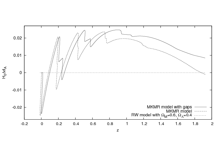
In our setting the MKMR model corresponds to $s_{\varsigma}=0.1$, $s_{a}=1$, $r_{b}=0.042$ and $\arg\sigma=\tilde{c}_{\phi}=0$ in each inhomogeneous region. We reproduced the result of [2007PhRvD..76l3004M]. The change in the angular diameter distance, $\Delta d_{A}(z)=d_{A}(z)-d_{A}(z)|_{RW}$, compared to the RW model with $\Omega_{M}=0.6$ and $\Omega_{\Lambda}=0.4$ is presented in Fig. 1. It coincides with Fig. $13$ in [2007PhRvD..76l3004M].

In the MKMR model, the light propagates radially in each coordinate patch. Since the mass is concentrated in spherical shells and the density in the central part of the inhomogeneity is tiny, the beam travels through regions with lower density than the average. The angular diameter distance in such model should deviate from the EdS value as it already follows from the weak lensing analysis. It seems interesting to calculate the angular diameter distance for more typical beams, i.e. the beams that are not so much statistically distinguished. Such analysis requires the study of non-radial beams and randomization of the sequence of impact parameters. This extension of the MKMR is not a trivial one and leads to some subtle problems that will be addressed in this Subsection.

Firstly, for non-radial beams an impact parameter takes random values in each inhomogeneous region and centres of those regions are not lined up any more. Clearly, gaps between inhomogeneities and an upper limit for an impact parameter are necessary to avoid overlapping of inhomogeneities. Gaps are introduced by setting $s_{a}=1.19048$ which implies $r_{a}=0.05$. In addition, we assume that the absolute value of the impact parameter is not larger than $\tilde{c}_{\phi}^{*}=0.84$ (as defined in the equation (13)). This assumption improves statistical properties of our models because it assures that the beam enters an inhomogeneous region in each coordinate patch.

Secondly, one has to decide how inhomogeneities are distributed in the spacetime. This is defined by the statistical properties of the sequence of impact parameters. We consider two possibilities in our paper. The spatial average density of the $t=const$ hypersurfaces does not deviate much from the EdS value. Hence, the natural assumption is that the average density along the beam which goes through inhomogeneous regions should not deviate from the average density along the beam that propagates in the EdS spacetime.¹⁰¹⁰ 10 We acknowledge private communication with Syksy Räsänen and Krzysztof Bolejko. See also [2011MNRAS.tmp...25B]. To achieve this, impact parameters are distributed in $[-\tilde{c}_{\phi}^{*},\tilde{c}_{\phi}^{*}]$ with the probability distribution function $|\tilde{c}_{\phi}/\tilde{c}_{\phi}^{*}|$. Such the probability distribution function corresponds to the trajectory of the typical beam that travels through inhomogeneous regions which are spread randomly in the spacetime.¹¹¹¹ 11 The finite size of inhomogeneities and the assumption that the beam should enter an inhomogeneous region in each coordinate patch imply that the distribution of centres of inhomogeneities in spacetime is not uniform. The second possibility we consider is that centres of all inhomogeneous regions are spread randomly in a plane and that the beam propagates in this plane. We will call this version of our models “aligned” and we will refer to remaining our models as to “non-aligned”. It is assumed that the typical beam in the plane with aligned inhomogeneities corresponds to the sequence of impact parameters uniformly distributed in the interval $[-\tilde{c}_{\phi}^{*},\tilde{c}_{\phi}^{*}]$. In our setting, this implies that the light propagates through regions with lower average density than the spatial average density in the model. Such configuration of inhomogeneities is unnatural, but it is convenient to model the selection effect, i.e. the light from the sources that are observed is more likely to travel through low density regions.

Next, the problem that is sometimes not handled properly in the literature is the value of shear at the boundary between coordinate patches. In general, the principal axes of shear do not have to coincide with our choice of Sachs basis. The rotation of principal axes of shear is necessary in non-aligned models and may be realised by a random change of the phase of shear ($\arg\sigma$) with the uniform probability distribution in $(-\pi,\pi]$. In aligned models, one should assume that the phase of shear do not change between coordinate patches. For a sake of curiosity, we will also consider the third possibility: an aligned model (a vanishing phase of shear) with the impact parameters probability distribution function $|\tilde{c}_{\phi}/\tilde{c}_{\phi}^{*}|$.

In the remaining part of the paper, the following terminology will be used. Whenever we will refer to the aligned version of the non-radial SC model, we will explicitly indicate that. We will also explicitly indicate whenever only radial beams will be studied in the model (if different than the MKMR model). The remaining models are assumed to be non-aligned and to contain non-radial beams.

Let us start with applying the extension presented in this Subsection to the MKMR model. In the first step we add gaps. The angular diameter – redshift curve in the radial MKMR model with gaps does not reveal big changes — Fig. 1. The inhomogeneities appear for a little bigger redshift, as expected.

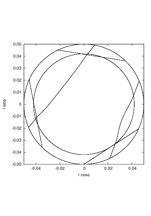
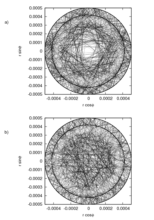
Next, we randomize impact parameters. The non-radial beams in the MKMR model with gaps are curved. We present them in Fig. 2, where $\tilde{c}_{\phi}$ is distributed in $[-\tilde{c}_{\phi}^{*},\tilde{c}_{\phi}^{*}]$ with the probability density $|\tilde{c}_{\phi}/\tilde{c}_{\phi}^{*}|$ (non-aligned setting). The angular diameter distance is lower than in the EdS model because the beam spends “more time” in the region of higher density — Fig. 3. The effect of inhomogeneities on the angular diameter distance is opposite than for radial beams. However, this is not a typical property of non-radial beams, but an effect of week randomization (only five inhomogeneous regions).

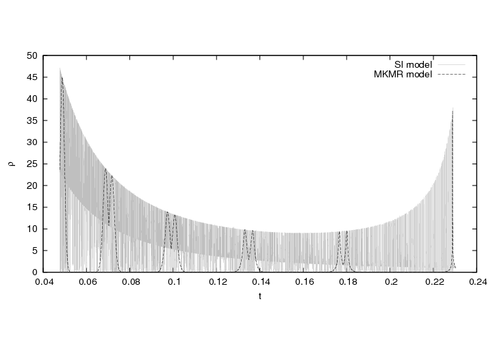
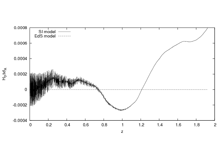
In the MKMR model with gaps (non-radial), the angular diameter distance $d_{A}(z)$ depends strongly on the sequence of impact parameters. One should average $d_{A}(z)$ over many runs to obtain a reliable result (like in [Vanderveld:2008vi]) or reduce the size of inhomogeneities to obtain the better statistic in a single run. We decided to reduce the size of inhomogeneities $100$ times (we set $r_{b}=0.00042$).¹²¹² 12 The diameter of the inhomogeneous region is around $10$ Mpc at the moment of an observation. In the model with small inhomogeneous regions (hereafter, the SI model), the density along the beam is a fast varying function — Fig. 5. For radial beams, the angular diameter distance does not change much, but in a general case the effect of inhomogeneities on the angular diameter distance is negligible — Figs 3, 5. For non-radial beams in the aligned SI model, the effect of inhomogeneities on light propagation for $z<1.5$ is lower than $10\%$ of what is needed to explain the accelerated expansion without introducing the cosmological constant. It is around one-third of the effect in the original MKMR model. Since this is the maximal effect we have observed in our models (after randomization of the trajectory of the beam), the aligned SI model corresponds to our “extremal” setting. The empty beam formula (26) gives the largest angular diameter distance.

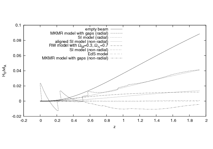
The typical trajectories in the SI model (non-aligned and aligned) are presented in Fig. 6. It follows from Figs 3, 5 that the effect of inhomogeneities on the angular diameter distance is reduced in our models to the insignificant level by proper randomization of the beam’s trajectory.

In the previous subsections, we have introduced non-radial beams with non-vanishing shear along the trajectories. In most models studied in the literature (including [Vanderveld:2008vi]), shear is assumed to be negligible for the angular diameter distance – redshift relation. We have verified that this is indeed true in our models.

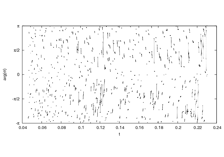
In the non-aligned models, the angle between Sachs basis and principal axes of shear is uncorrelated between inhomogeneous regions (Fig. 8). In contrast to that, in the aligned models the phase of shear is constant and equal to zero.

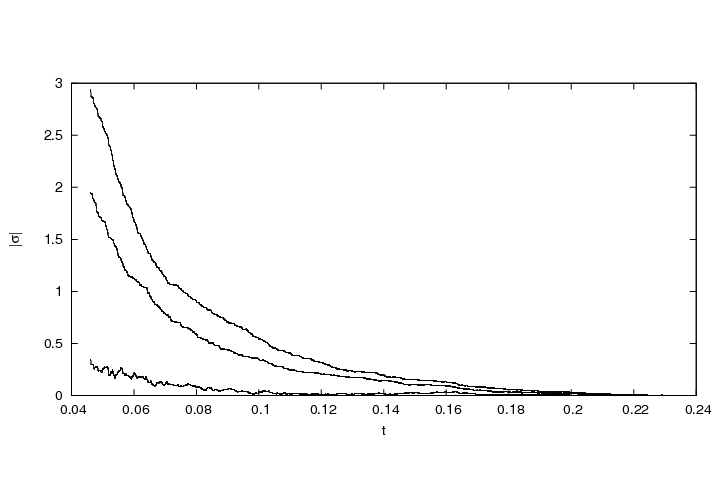
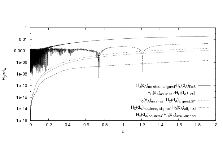
We compare the value of shear in three versions of the SI models: non-aligned, aligned, and aligned (a vanishing phase of shear) with the probability distribution function of the impact parameters $|\tilde{c}_{\phi}/\tilde{c}_{\phi}^{*}|$. The last model was introduced to verify validity of some calculations presented in the literature. It will be distinguished with a symbol SI*. The modulus of shear is a smooth function and is presented in Fig. 8. It is interesting to observe in this figure the averaging effect of non-aligned inhomogeneities on shear.

Let $n$ be a number of inhomogeneous regions encountered by the beam. At first sight the non-aligned positions of inhomogeneities (in the non-aligned SI model) lead to a random walk in $|\sigma|\sim\sqrt{n}$ in contrast to the aligned case where $|\sigma|\sim n$ (the aligned SI model). We have verified that the curves in Fig. 8 do not satisfy this relations. Since structures are growing in time, the expected value of the change of shear between neighbouring inhomogeneities is time dependent. Therefore, this process may be studied as a continuous time random walk.

In Fig. 9 we present the difference of the angular diameter distances between the SI model, the aligned SI model, the aligned SI* model and the SI model with neglected shear (non-aligned and aligned), and the EdS model. This comparison reveals that the effect of shear for non-aligned SI models is tiny (for $z=1.5$ it less than $0.1\%$ of the correction to the EdS angular diameter distance). For aligned SI models, it is less than $1\%$ (for $z=1.5$). However, the aligned SI* model (with the probability distribution function $|\tilde{c}_{\phi}/\tilde{c}_{\phi}^{*}|$), overestimate it around two orders of magnitude (for $z=1.5$ the effect of shear is around $10\%$ of the correction to the EdS angular diameter distance).

The random number generator in our code was initialized with the same random seed. Therefore, three bottom curves in Fig. 9 are not jagged for small redshifts.

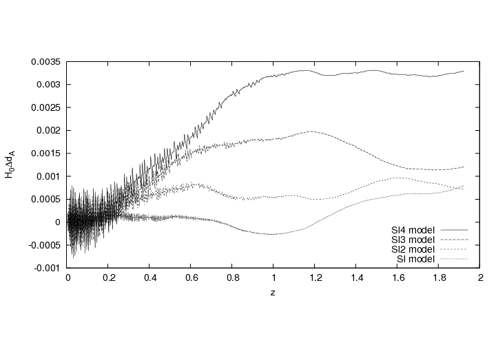
It was argued in [Vanderveld:2008vi] that the dimming of supernovae in the MKMR model may be roughly estimated with a help of the partially filled beam approximation (26). We apply this approximation to five models: the SI model, three SIn models with inhomogeneities n-times bigger than in the SI model (where $n=2,3,4$), and the MKMR model. The angular diameter distance, in variations of the SI model, seems to depend slightly on the size of inhomogeneities (Fig. 10) and the sequence of impact parameters induces big statistical fluctuations.¹³¹³ 13 The code was initialized with the same random seed, but sizes of inhomogeneities are different. Therefore, the different parts of a random sequence corresponds to different redshifts.

We suppose that it is not size of inhomogeneities that matters, but randomization, i.e. how the average density along the beam deviates from the EdS value.¹⁴¹⁴ 14 The radial versions of MKMR and SI models give similar angular diameter distance as may be seen in Fig. 3. This may be seen as follows. Let us calculate the smoothness parameter $\tilde{\alpha}$ for each model. The smoothness parameter is a mass-fraction of the matter in the Universe that is not bounded in galaxies. We calculate it for our SC models using

$$\tilde{\alpha}=\frac{1}{\lambda_{0}-\lambda_{S}}\int_{\lambda_{0}}^{\lambda_{S}}\frac{\rho_{SC}(\lambda)}{\rho_{EdS}(t_{SC}(\lambda))}d\lambda\;,$$

(30)

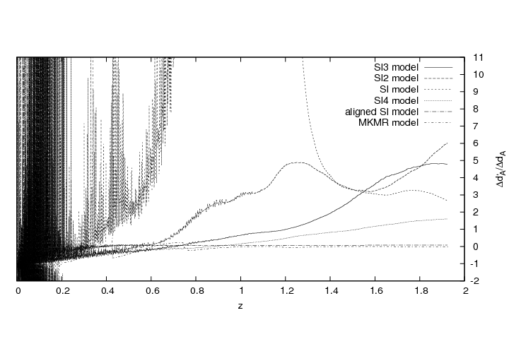
where $\lambda_{0}=0$ denotes an affine parameter at the observer and $\lambda_{S}$ corresponds to the emission. In our models, the spatial average density of the $t=const$ hypersurfaces is approximately equal to the density in the EdS model. Therefore, one may expect that $\tilde{\alpha}$ should not diverge far from $1$. However, the bigger are inhomogeneities, the weaker is randomization of the path of the beam. Since low density regions occupy larger volume in the studied models, it is more likely that $\tilde{\alpha}$ will decrease with increasing size of inhomogeneities (the variance will grow). We have found $\tilde{\alpha}$ to be approximately equal to $0.964$, $0.939$, $0.915$, $0.895$, $0.815$, $0.412$ for the SI, SI2, SI3, SI4, aligned SI, MKMR models, respectively. For SI models that contain hundreds of inhomogeneities, $\tilde{\alpha}$ is slightly lower than $1$. The values of $\tilde{\alpha}$ for particular models together with Fig. 10 suggest that the effect of inhomogeneities on the angular diameter distance depends on the average density along the beam (as expected from the week lensing approximation).

We plotted Fig. 11 which shows the difference between the partially filled beam formula and the numerical result for the approximated model. It reveals that the partially filled beam approximation is acceptable for smaller values of $\tilde{\alpha}$. The accuracy is around $1\%$ of the correction to the EdS angular diameter distance for the MKMR model and $8\%$ for the aligned SI model (for $z=1.5$). In our models, the partially filled beam approximation does not work for larger values¹⁵¹⁵ 15 For $\tilde{\alpha}\simeq 1$, the effect of inhomogeneities seems to be smaller than statistical fluctuations. of $\tilde{\alpha}$.