跳到论文正文
W Papers独立论文阅读器 arXiv:1012.5071 论文正文 计算阅读时间 · 0%
引用这篇论文根据当前论文元数据生成,正式投稿前建议核对。


License: arXiv.org perpetual non-exclusive license
arXiv:1012.5071v2 [cs.IT] 27 Dec 2010

Extension of the Blahut-Arimoto algorithm for maximizing directed information

Iddo Naiss    Haim Permuter ††thanks: Iddo Naiss and Haim Permuter are with the Department of Electrical and Computer Engineering, Ben-Gurion University of the Negev, Beer-Sheva, Israel. Emails: naiss@bgu.ac.il, haimp@bgu.ac.il.
Abstract

We extend the Blahut-Arimoto algorithm for maximizing Massey’s directed information. The algorithm can be used for estimating the capacity of channels with delayed feedback, where the feedback is a deterministic function of the output. In order to do so, we apply the ideas from the regular Blahut-Arimoto algorithm, i.e., the alternating maximization procedure, onto our new problem. We provide both upper and lower bound sequences that converge to the optimum value. Our main insight in this paper is that in order to find the maximum of the directed information over causal conditioning probability mass function (PMF), one can use a backward index time maximization combined with the alternating maximization procedure. We give a detailed description of the algorithm, its complexity, the memory needed, and several numerical examples.

Index Terms: 
Alternating maximization procedure, Backwards index time maximization, Blahut-Arimoto algorithm, Causal conditioning, Channels with feedback, Directed information, Finite state channels, Ising Channel, Trapdoor channel.

I Introduction

In his seminal work, Shannon [1] showed that the capacity of a memoryless channel is given as the optimization problem

C=maxp⁡(x)⁡I⁡(X,Y).\displaystyle C=\max_{p(x)}{I(X;Y)}. (1)

Since the set of all p⁡(x)p(x) is not of finite cardinality, an optimization method is required to find the capacity CC. In order to obtain an efficient way to calculate the global maximum in (1), the well-known Blahut-Arimoto algorithm (referred to as BAA) was introduced by Blahut [2] and Arimoto [3] in 1972. The main idea is that we can calculate the optimum value using the equality

maxp⁡(x)⁡I⁡(X,Y)=maxp⁡(x),p⁡(x|y)⁡I⁡(X,Y),\max_{p(x)}I(X;Y)=\max_{p(x),p(x|y)}I(X;Y),

i.e., we can maximize over p⁡(x)p(x) and p⁡(x|y)p(x|y), instead of just p⁡(x)p(x) alone. The maximization is then achieved using the alternating maximization procedure. The convergence of the alternating maximization procedure to the global maximum was proven by Csiszar and Tusnady [4], and later by Yeung [5].

In this paper, we find an efficient way to estimate the capacity of channels with feedback. It was shown by Massey [6], Kramer [7], Tatikonda and Mitter[8], Permuter, Weissman, and Goldsmith [9], and Kim [10], that the expression

Cn=1nmaxp(xn||yn−1)I(Xn→Yn)\displaystyle C_{n}=\frac{1}{n}\max_{p(x^{n}||y^{n-1})}I(X^{n}\rightarrow Y^{n})

has an important role in characterizing the feedback capacity, where

I⁡(Xn→Yn)\displaystyle I(X^{n}\rightarrow Y^{n}) =∑yn,xnp⁡(yn,xn)​log⁡p(yn||xn)p⁡(yn)\displaystyle=\sum_{y^{n},x^{n}}{p(y^{n},x^{n})\log{\frac{p(y^{n}||x^{n})}{p(y^{n})}}}

is the directed information, and p(yn||xn)p(y^{n}||x^{n}) is a causally conditioned PMF (definitions in Section II) given by

p(yn||xn)=∏i=1np(yi|yi−1,xi).\displaystyle p(y^{n}||x^{n})=\prod_{i=1}^{n}{p(y_{i}|y^{i-1},x^{i})}. (2)

Since in the maximization we deal with causally conditioned PMFs, trying to follow the regular BAA will result in difficulties. This is due to the fact that a causal conditioned PMF is the result of multiplications of conditioned PMFs as seen in (2). While in the regular BAA we maximize over p⁡(xn)p(x^{n}), and thus the constraints are simply ∑xnp⁡(xn)=1\sum_{x^{n}}p(x^{n})=1 and p⁡(xn)≥0p(x^{n})\geq 0, in our extended problem we have no efficient way of writing all the constraints necessary for a causally conditioned PMF. In fact, we need nn simple constraints, one for each product of p(xn||yn−1)p(x^{n}||y^{n-1}). Another difficulty is that although the equality

I(Xn→Yn)=∑i=1nI(Xi;Yin|Xi−1,Yi−1)\displaystyle I(X^{n}\rightarrow Y^{n})=\sum_{i=1}^{n}I(X_{i};Y_{i}^{n}|X^{i-1},Y^{i-1})

holds, we cannot translate the given problem into

∑i=1nmaxp⁡(xi|xi−1,yi−1)I(Xi;Yin|Xi−1,Yi−1)\displaystyle\sum_{i=1}^{n}\max_{p(x_{i}|x^{i-1},y^{i-1})}I(X_{i};Y_{i}^{n}|X^{i-1},Y^{i-1})

since p⁡(xi|xi−1,yi−1)p(x_{i}|x^{i-1},y^{i-1}) influence all terms {I(Xj;Yjn|Xj−1,Yj−1)}j=in\{I(X_{j};Y_{j}^{n}|X^{j-1},Y^{j-1})\}_{j=i}^{n}. A solution could be to maximize backwards from i=ni=n to i=1i=1 over p⁡(xi|xi−1,yi−1)p(x_{i}|x^{i-1},y^{i-1}), and it can be shown that in each maximization, the non-causal probability p⁡(xi|xi−1,yn)p(x_{i}|x^{i-1},y^{n}) is determined only by the previous p⁡(xj|xj−1,yj−1)p(x_{j}|x^{j-1},y^{j-1}) for j≥ij\geq i. In our solution, we maximize the entire expression I⁡(Xn→Yn)I(X^{n}\rightarrow Y^{n}) as a function of {p⁡(x1),p⁡(x2|x1,y1),…,p⁡(xn|xn−1,yn−1),p⁡(xn|yn)}\{p(x_{1}),p(x_{2}|x_{1},y_{1}),...,p(x_{n}|x^{n-1},y^{n-1}),p(x^{n}|y^{n})\}. Each time we maximize over a specific p⁡(xi|xi−1,yi−1)p(x_{i}|x^{i-1},y^{i-1}) starting from i=ni=n and moving backwards to i=1i=1, where all but p⁡(xi|xi−1,yi−1)p(x_{i}|x^{i-1},y^{i-1}) are fixed.

Before we present the extension of the BAA to the directed information, let us present some of the other extensions of this algorithm. In 2004, Matz and Duhamel[11] proposed two Blahut-Arimoto-type algorithms that often converge significantly faster than the standard Blahut-Arimoto algorithm, which relied on following the natural gradient rather than maximizing per variable. During that year, Rezaeian and Grant [12] generalized the regular BAA for multiple access channels, and Dupuis, Yu, and Willems extended the BAA for channels with side information [13]. They used the fact that the input is a deterministic function of the auxiliary variable and the side information, and then extended the input alphabet. Another solution to the side information problem was given by El Gamal and Heegard[14], where they did not expand the alphabet, but included an additional step to optimize over p⁡(x|u,s)p(x|u,s). Also, the BAA was used by Egorov, Markavian, and Pickavance [15] to decode Reed Solomon codes. In 2005 Dauwels [16] showed how the BAA can be used to calculate the capacity of continuous channels. Dauwels’s main idea is the use of sequential Monte-Carlo integration methods known as the ”particle filters”. In 2008 Vontobel, Kavc̆ić, Arnold, and Loeliger[17] extended the regular BAA to estimate the capacity of finite state channels where the input is Markovian. Sumszyk and Steinberg [18] gave a single letter characterization of the capacity of an information embedding channel and provided a BA-type algorithm for the case where the channel is independent of the host given the input.

Recently, few papers about the maximization of the directed information using control theory and dynamic programming were published. In [19], Yang, Kavcic and Tatikonda maximized the directed information to estimate the feedback capacity of finite-state machine channels where the state is a deterministic function of the previous state and input. Chen and Berger [20] maximized the directed information for the case where the state of the channel is known to the encoder and decoder in addition to the feedback link. Later, Permuter, Cuff, Van Roy and Weissman [21] maximized the directed information and found the capacity of the trapdoor channel with feedback. In [22], Gorantla and Coleman estimated the maximum of directed information where they considered a dynamical system, whose state is an input to a memoryless channel. The state of the dynamical system is affected by its past, an exogenous input, and causal feedback from the channel’s output.

The remainder of the paper is organized as follows. In Section II we present the notations we use throughout the paper, and give the outline for the alternating maximization procedure as given by Yeung[5]. In Section III we give a description of the algorithm for solving the optimization problem- maxp(xn||yn−1)I(Xn→Yn)\max_{p(x^{n}||y^{n-1})}I(X^{n}\rightarrow Y^{n}), calculate the complexity of the algorithm and memory needed, and compare it with those of the regular BAA. In Section IV we derive the algorithm using the alternating maximization procedure, and show the convergence of our algorithm to the optimum value. Numerical examples for channel capacity with feedback are presented in Section V. In Appendix A we give a wider angle on the feedback channel problem, where the feedback of the channel is a deterministic function ff of the output with some delay dd; namely, we derive the algorithm for the optimization problem maxp(xn||zn−d)I(Xn→Yn),\max_{p(x^{n}||z^{n-d})}I(X^{n}\rightarrow Y^{n}), where zi=f⁡(yi)z_{i}=f(y_{i}) and d≥1d\geq 1. In Appendix B we prove an upper bound for maxp(xn||yn−d)I(Xn→Yn),\max_{p(x^{n}||y^{n-d})}I(X^{n}\rightarrow Y^{n}), which converges to the directed information from above and helps determining the stoping iteration of the algorithm.

II Preliminaries

II-A Directed information and causal conditioning

In this section we present the definitions of directed information and causally conditioned PMF, originally introduced by Massey[6] (who was inspired by Marko’s work [23] on Bidirectional Communication) and by Kramer [7]. These definitions are necessary in order to address channels with memory. We denote by X1nX_{1}^{n} the vector (X1,X2,…​Xn)(X_{1},X_{2},...X_{n}). Usually we use the notation Xn=X1nX^{n}=X_{1}^{n} for short. Further, when writing a PMF we simply write PX​(X=x)=p⁡(x)P_{X}(X=x)=p(x). Let us denote as p(xn||yn−d)p(x^{n}||y^{n-d}) the probability mass function (PMF) of XnX^{n} causally conditioned on Yn−dY^{n-d}, given by

p(xn||yn−d)≜∏i=1np(xi|xi−1yi−d).\displaystyle p(x^{n}||y^{n-d})\triangleq\prod^{n}_{i=1}{p(x_{i}|x^{i-1}y^{i-d})}. (3)

Here we have to establish that when d>nd>n, the vector Xn−d=∅X^{n-d}=\emptyset. Two straight forward properties of the causal conditioning PMF that we use throughout the paper are

∑xnp(xn||yn−d)=p(xn−1||yn−d−1),\displaystyle\sum_{x_{n}}p(x^{n}||y^{n-d})=p(x^{n-1}||y^{n-d-1}), (4)

and

p⁡(xi|xi−1​yi−d)=p(xi||yi−d)p(xi−1||yi−d−1).\displaystyle p(x_{i}|x^{i-1}y^{i-d})=\frac{p(x^{i}||y^{i-d})}{p(x^{i-1}||y^{i-d-1})}. (5)

Another elementary property is the chain rule for directed information

p(xn||yn−1)p(yn||xn)=p(xn,yn).\displaystyle p(x^{n}||y^{n-1})p(y^{n}||x^{n})=p(x^{n},y^{n}). (6)

The definitions above lead to the causally conditioned entropy H(Xn||Yn)H(X^{n}||Y^{n}), which is given by

H(Xn||Yn)≜−𝔼[logp(Xn||Yn)].H(X^{n}||Y^{n})\triangleq-\mathbb{E}\left[{\log p(X^{n}||Y^{n})}\right].

Moreover, the directed information from XnX^{n} to YnY^{n} is given by

I(Xn→Yn)≜H(Yn)−H(Yn||Xn).\displaystyle I(X^{n}\rightarrow Y^{n})\triangleq H(Y^{n})-H(Y^{n}||X^{n}). (7)

It is possible to show, that we can write the directed information as such:

I(Xn→Yn)=∑yn,xnp(yn||xn)r(xn||yn−1)logq⁡(xn|yn)r(xn||yn−1).\displaystyle I(X^{n}\rightarrow Y^{n})=\sum_{y^{n},x^{n}}{p(y^{n}||x^{n})r(x^{n}||y^{n-1})\log{\frac{q(x^{n}|y^{n})}{r(x^{n}||y^{n-1})}}}.

We refer to this form when using the alternating maximization procedure since {r=r(xn||yn−1),q=q(xn|yn)}\{\textbf{r}=r(x^{n}||y^{n-1}),\ \textbf{q}=q(x^{n}|y^{n})\} are the variables we optimize over where p(yn||xn)p(y^{n}||x^{n}) is fixed. For convenience, we use from now on the notation of

I⁡(Xn→Yn)=ℐ⁡(r,q)\displaystyle I(X^{n}\rightarrow Y^{n})=\cal{I}(\textbf{r},\textbf{q}) (8)

when required. With these definitions, we follow the alternating maximization procedure given by Yeung[5] in order to maximize the directed information.

II-B Alternating maximization procedure

Here, we present the alternating maximization procedure on which our algorithm is based. Let f⁡(u1,u2)f(u_{1},u_{2}) be a real function, and let us consider the optimization problem given by

supu1∈A1,u2∈A2f⁡(u1,u2)=f∗.\sup_{u_{1}\in A_{1},u_{2}\in A_{2}}f(u_{1},u_{2})=f^{*}.

We denote by c2​(u1)∈A2c_{2}(u_{1})\in A_{2} the point that achieves supu2∈A2f⁡(u1,u2)\sup_{u_{2}\in A_{2}}f(u_{1},u_{2}), and by c1​(u2)∈A1c_{1}(u_{2})\in A_{1} the one that achieves supu1∈A1f⁡(u1,u2)\sup_{u_{1}\in A_{1}}f(u_{1},u_{2}). The algorithm is defined by iterations, where in each iteration we maximize over one of the variables. Let (u10,u20)(u_{1}^{0},u_{2}^{0}) be an arbitrary point in A1×A2A_{1}\times A_{2}. For k≥0k\geq 0 let

(u1k,u2k)=(c1​(u2k−1),c2​(c1​(u2k−1))),(u_{1}^{k},u_{2}^{k})=(c_{1}(u_{2}^{k-1}),c_{2}(c_{1}(u_{2}^{k-1}))),

and let fk=f⁡(u1k,u2k)f^{k}=f(u_{1}^{k},u_{2}^{k}) be the value if the present iteration. The following lemma describes the conditions the problem needs to meet in order for fkf^{k} to converge to f∗f^{*} as kk goes to infinity.

Lemma 1 (Lemmas 9.4, 9.5 in [5], Convergence of the alternating maximization procedure)

. Let f⁡(u1,u2)f(u_{1},u_{2}) be a real, concave, bounded from above function that is continuous and has continuous partial derivatives, and let the sets A1,A2,A_{1},A_{2}, which we maximize over, be convex. Further, assume that c2​(u1)∈A2c_{2}(u_{1})\in A_{2} and c1​(u2)∈A1c_{1}(u_{2})\in A_{1} for all u1∈A1,u2∈A2u_{1}\in A_{1},\ u_{2}\in A_{2}. Under these conditions, limk→∞fk=f∗\lim_{k\rightarrow\infty}f^{k}=f^{*}.

In Section III we give a detailed description of the algorithm that computes maxp(xn||yn−1)I(Xn→Yn)\max_{p(x^{n}||y^{n-1})}I(X^{n}\rightarrow Y^{n}) based on the alternating maximization procedure. In Section IV we show that the conditions in Lemma 1 hold, and therefore the algorithm we suggest, which is based on the alternating maximization procedure, converges to the global optimum.

III Description of the algorithm

In this section, we describe an algorithm for maximizing the directed information. In addition, we compute the complexity of the algorithm per iteration, and compare it to the complexity of the regular BAA. The memory calculation is also given.

III-A The algorithm for channel with feedback

In Algorithm 1, we present the steps required to maximize the directed information where the channel p(yn||xn)p(y^{n}||x^{n}) is fixed and the delay is d=1d=1.

Algorithm 1 Iterative algorithm for calculating maxp(xn||yn−1)I(Xn→Yn)\max_{p(x^{n}||y^{n-1})}I(X^{n}\rightarrow Y^{n}), where p(yn||xn)p(y^{n}||x^{n}) is fixed.
  • (a)

    Start from a random point q⁡(xn|yn)q(x^{n}|y^{n}). Usually we start from a uniform distribution, i.e., q⁡(xn|yn)=2−nq(x^{n}|y^{n})=2^{-n} for every (xn,yn)(x^{n},y^{n})

  • (b)

    Starting from i=ni=n, calculate r⁡(xi|xi−1,yi−1)r(x_{i}|x^{i-1},y^{i-1}) using the formula

    r⁡(xi|xi−1,yi−1)=r′​(xi,yi−1)∑xir′​(xi,yi−1),r(x_{i}|x^{i-1},y^{i-1})=\frac{r^{\prime}(x^{i},y^{i-1})}{\sum_{x_{i}}r^{\prime}(x^{i},y^{i-1})}, (9)

    where

    r′​(xi,yi−1)=∏xi+1n,yin[q⁡(xn|yn)∏j=i+1nr⁡(xj|xj−1,yj−1)]p⁡(yi|xi,yi−1)​∏j=i+1nr⁡(xj|xj−1,yj−1)​p​(yj|xj,yj−1),r^{\prime}(x^{i},y^{i-1})=\prod_{x_{i+1}^{n},y_{i}^{n}}{\left[\frac{q(x^{n}|y^{n})}{\prod_{j=i+1}^{n}{r(x_{j}|x^{j-1},y^{j-1})}}\right]^{p(y_{i}|x^{i},y^{i-1})\prod_{j=i+1}^{n}{r(x_{j}|x^{j-1},y^{j-1})p(y_{j}|x^{j},y^{j-1})}}}, (10)

    and do so backwards until i=1i=1.

  • (c)

    Once you have r⁡(xi|xi−1,yi−1)r(x_{i}|x^{i-1},y^{i-1}) for all i∈{1,…,n}i\in\{1,...,n\}, compute r(xn||yn−1)=∏i=1nr(xi|xi−1,yi−1)r(x^{n}||y^{n-1})=\prod_{i=1}^{n}{r(x_{i}|x^{i-1},y^{i-1})}.

  • (d)

    Compute q⁡(xn|yn)q(x^{n}|y^{n}) using the formula

    q⁡(xn|yn)=r(xn||yn−1)p(yn||xn)∑xnr(xn||yn−1)p(yn||xn).q(x^{n}|y^{n})=\frac{r(x^{n}||y^{n-1})p(y^{n}||x^{n})}{\sum_{x^{n}}{r(x^{n}||y^{n-1})p(y^{n}||x^{n})}}. (11)
  • (e)

    Calculate IU−ILI_{U}-I_{L}, where

    IL\displaystyle I_{L} =1n∑yn,xnp(yn||xn)r(xn||yn−1)logq⁡(xn|yn)r(xn||yn−1),\displaystyle=\frac{1}{n}\sum_{y^{n},x^{n}}{p(y^{n}||x^{n})r(x^{n}||y^{n-1})\log{\frac{q(x^{n}|y^{n})}{r(x^{n}||y^{n-1})}}},
    IU\displaystyle I_{U} =1nmaxx1∑y1maxx2⋯∑yn−1maxxn∑ynp(yn||xn)logp(yn||xn)∑x′np(yn||x′n)⋅r(x′n||yn−1).\displaystyle=\frac{1}{n}\max_{x_{1}}\sum_{y_{1}}\max_{x_{2}}\cdots\sum_{y_{n-1}}\max_{x_{n}}\sum_{y_{n}}p(y^{n}||x^{n})\log\frac{p(y^{n}||x^{n})}{\sum_{x^{\prime n}}p(y^{n}||x^{\prime n})\cdot r(x^{\prime n}||y^{n-1})}.
  • (f)

    Return to (b) if (IU−IL)≥ϵ(I_{U}-I_{L})\geq\epsilon.

  • (g)

    Cn=ILC_{n}=I_{L}.

Note that the regular BAA has a structure similar to that of Algorithm 1, where step (b) is an additional backward loop. Its purpose is to maximize over the input causal probability, which is not necessary in the regular BAA.

Now, let us present a special case and a few extensions for Alg. 1.

  • (1)

    Regular BAA, i.e., n=1n=1. For n=1n=1, the algorithm suggested here agrees with the original BAA, where instead of steps (b), (c) we have

    r⁡(x)=∏yq​(x|y)p⁡(y|x)∑x∏yq​(x|y)p⁡(y|x),\displaystyle r(x)=\frac{\prod_{y}{q(x|y)^{p(y|x)}}}{\sum_{x}\prod_{y}q(x|y)^{p(y|x)}}, (12)

    and step (d) is replaced by

    q⁡(x|y)=r⁡(x)​p​(y|x)∑xr⁡(x)​p​(y|x).\displaystyle q(x|y)=\frac{r(x)p(y|x)}{\sum_{x}{r(x)p(y|x)}}. (13)

    The bounds IL,IUI_{L},\ I_{U} agree with the regular BAA as well, and are of the form

    IL\displaystyle I_{L} =∑y,xp⁡(y|x)​r​(x)​log⁡q⁡(x|y)r⁡(x),\displaystyle=\sum_{y,x}{p(y|x)r(x)\log{\frac{q(x|y)}{r(x)}}},
    IU\displaystyle I_{U} =max⁡∑yx⁡p⁡(y|x)​log⁡p⁡(y|x)∑x′p⁡(y|x′)⋅r⁡(x′).\displaystyle=\max_{x}\sum_{y}p(y|x)\log\frac{p(y|x)}{\sum_{x^{\prime}}p(y|x^{\prime})\cdot r(x^{\prime})}.
  • (2)

    Feedback with general delay dd. We can generalize the algorithm in order to compute maxr(xn||yn−d)I(Xn→Yn)\max_{r(x^{n}||y^{n-d})}I(X^{n}\rightarrow Y^{n}), where the feedback is the output with delay dd. In that case, in step (b) we have

    r′​(xi,yi−d)=∏xi+1n,yi−d+1n[q⁡(xn|yn)∏j=i+1nr⁡(xj|xj−1,yj−d)]∏j=i−d+1np⁡(yj|xj,yj−1)​∏j=i+1nr⁡(xj|xj−1,yj−d),\displaystyle r^{\prime}(x^{i},y^{i-d})=\prod_{x_{i+1}^{n},y_{i-d+1}^{n}}{\left[\frac{q(x^{n}|y^{n})}{\prod_{j=i+1}^{n}{r(x_{j}|x^{j-1},y^{j-d})}}\right]^{\prod_{j=i-d+1}^{n}{p(y_{j}|x^{j},y^{j-1})}\prod_{j=i+1}^{n}{r(x_{j}|x^{j-1},y^{j-d})}}}, (14)

    and step (d) will be replaced by

    q⁡(xn|yn)=r(xn||yn−d)p(yn||xn)∑xnr(xn||yn−d)p(yn||xn).\displaystyle q(x^{n}|y^{n})=\frac{r(x^{n}||y^{n-d})p(y^{n}||x^{n})}{\sum_{x^{n}}{r(x^{n}||y^{n-d})p(y^{n}||x^{n})}}. (15)

    The bounds IL,IUI_{L},\ I_{U} are of the form

    IL\displaystyle I_{L} =1n∑yn,xnp(yn||xn)r(xn||yn−d)logq⁡(xn|yn)r(xn||yn−d),\displaystyle=\frac{1}{n}\sum_{y^{n},x^{n}}{p(y^{n}||x^{n})r(x^{n}||y^{n-d})\log{\frac{q(x^{n}|y^{n})}{r(x^{n}||y^{n-d})}}},
    IU\displaystyle I_{U} =1nmaxxd∑y1maxxd+1⋯∑yn−dmaxxn∑yn−d+1np(yn||xn)logp(yn||xn)∑x′np(yn||x′n)⋅r(x′n||yn−d).\displaystyle=\frac{1}{n}\max_{x^{d}}\sum_{y_{1}}\max_{x_{d+1}}\cdots\sum_{y_{n-d}}\max_{x_{n}}\sum_{y_{n-d+1}^{n}}p(y^{n}||x^{n})\log\frac{p(y^{n}||x^{n})}{\sum_{x^{\prime n}}p(y^{n}||x^{\prime n})\cdot r(x^{\prime n}||y^{n-d})}.
  • (3)

    Feedback as a function of the output with general delay. In Appendix A, we generalize the algorithm in order to compute maxr(xn||zn−d)I(Xn→Yn)\max_{r(x^{n}||z^{n-d})}I(X^{n}\rightarrow Y^{n}), where the feedback zn−dz^{n-d} is a deterministic function of the delayed output. The expression characterizes the capacity of channels with time-invariant feedback[9]. In that case, in step (b) we have

    r′​(xi,zi−d)=∏xi+1n,yi−d+1n∏Ai,d,z[q⁡(xn|yn)∏j=i+1nr⁡(xj|xj−1,zj−d)]p(yn||xn)∏j=i+1nr(xj|xj−1,zj−d)∑Ai,d,z∏j=1i−dp⁡(yj|xj,yj−1),\displaystyle r^{\prime}(x^{i},z^{i-d})=\prod_{x_{i+1}^{n},y_{i-d+1}^{n}}\prod_{A_{i,d,z}}{\left[\frac{q(x^{n}|y^{n})}{\prod_{j=i+1}^{n}{r(x_{j}|x^{j-1},z^{j-d})}}\right]^{\frac{p(y^{n}||x^{n})\prod_{j=i+1}^{n}{r(x_{j}|x^{j-1},z^{j-d})}}{\sum_{A_{i,d,z}}\prod_{j=1}^{i-d}{p(y_{j}|x^{j},y^{j-1})}}}}, (16)

    where we define the set Ai,d,z≜{yi−d:zi−d=f⁡(yi−d)}A_{i,d,z}\triangleq\{y^{i-d}:z^{i-d}=f(y^{i-d})\} as the set of output sequences that ff transforms to zi−dz^{i-d}, and step (d) will be replaced by

    q⁡(xn|yn)=r(xn||zn−d)p(yn||xn)∑xnr(xn||zn−d)p(yn||xn).\displaystyle q(x^{n}|y^{n})=\frac{r(x^{n}||z^{n-d})p(y^{n}||x^{n})}{\sum_{x^{n}}{r(x^{n}||z^{n-d})p(y^{n}||x^{n})}}. (17)

    The bounds IL,IUI_{L},\ I_{U} are of the form

    IL\displaystyle I_{L} =1n∑yn,xnp(yn||xn)r(xn||zn−d)logq⁡(xn|yn)r(xn||zn−d),\displaystyle=\frac{1}{n}\sum_{y^{n},x^{n}}{p(y^{n}||x^{n})r(x^{n}||z^{n-d})\log{\frac{q(x^{n}|y^{n})}{r(x^{n}||z^{n-d})}}},
    IU\displaystyle I_{U} =1nmaxxd∑z1maxxd+1⋯∑zn−dmaxxn∑An,d,z∑yn−d+1np(yn||xn)logp(yn||xn)∑x′np(yn||x′n)⋅r(x′n||zn−d).\displaystyle=\frac{1}{n}\max_{x^{d}}\sum_{z_{1}}\max_{x_{d+1}}\cdots\sum_{z_{n-d}}\max_{x_{n}}\sum_{A_{n,d,z}}\sum_{y_{n-d+1}^{n}}p(y^{n}||x^{n})\log\frac{p(y^{n}||x^{n})}{\sum_{x^{\prime n}}p(y^{n}||x^{\prime n})\cdot r(x^{\prime n}||z^{n-d})}.

Note, that for d=nd=n, the vector zn−d=∅z^{n-d}=\emptyset, hence r⁡(xi|xi−1,zi−d)=r⁡(xi|xi−1)r(x_{i}|x^{i-1},z^{i-d})=r(x_{i}|x^{i-1}), and

r(xn||zn−d)=∏i=1nr(xi|xi−1)=r(xn).r(x^{n}||z^{n-d})=\prod_{i=1}^{n}r(x_{i}|x^{i-1})=r(x^{n}).

Also note that when f⁡(y)=c​o​n​s​tf(y)=const, r(xn||zn−d)=r(xn)r(x^{n}||z^{n-d})=r(x^{n}), Ai,d,z=yi−dA_{i,d,z}=y^{i-d}, and ∑yi−d∏j=1i−dp⁡(yj|xj,yj−1)=1\sum_{y^{i-d}}\prod_{j=1}^{i-d}{p(y_{j}|x^{j},y^{j-1})}=1. In each of the cases above (d=nd=n or f⁡(y)=c​o​n​s​t.f(y)=const.), in step (d) we have

q⁡(xn|yn)=r(xn)p(yn||xn)∑xnr(xn)p(yn||xn),q(x^{n}|y^{n})=\frac{r(x^{n})p(y^{n}||x^{n})}{\sum_{x^{n}}{r(x^{n})p(y^{n}||x^{n})}},

and we obtain a different version of the regular BAA for channel capacity, where the maximization is done over all r⁡(xi|xi−1)r(x_{i}|x^{i-1}) instead of over r⁡(xn)r(x^{n}) at once. Furthermore, if f⁡(y)=yf(y)=y then case (3) agrees with all the equations of case (2).

III-B Complexity and Memory needed

Here, we give an expression for the computation complexity of one iteration in the algorithm, and then compare it to regular BAA. This will be done in two parts, one for each step in the iteration.

  • (1)

    Complexity of computing q⁡(xn|yn)q(x^{n}|y^{n}) as given in (11). For each yny^{n}, we need |𝒳|n{|\cal{X}|}^{n} multiplications for a specific xnx^{n} and use the denominator computed for every other xnx^{n}, thus obtaining O⁡(|𝒳|n)O({|\cal{X}|}^{n}) operations. Doing so for all yny^{n} achieves O⁡(|𝒳|n​|𝒴|n)=O⁡((|𝒳|​|𝒴|)n)O({|\cal{X}|}^{n}{|\cal{Y}|}^{n})=O({(|\cal{X}||\cal{Y}|)}^{n}).

  • (2)

    Complexity of computing r(xn||yn−1)r(x^{n}||y^{n-1}). First, we compute the complexity of each r⁡(xi|xi−1,yi−1)r(x_{i}|x^{i-1},y^{i-1}) as given in (10), assuming that an exponent is a constant number of computations, i.e., O⁡(1)O(1). Simple computations will conclude that the entire numerator takes about O⁡((n−i)​(|𝒳|​|𝒴|)n−i)O((n-i){(|\cal{X}||\cal{Y}|)}^{n-i}) computations. The denominator is a summation over |𝒳|i{|\cal{X}|}^{i} variables, and as with q⁡(xn|yn)q(x^{n}|y^{n}), we can use the denominator for every other xix^{i}. Hence, we obtain O⁡((n−i)​(|𝒳|​|𝒴|)n)O((n-i){(|\cal{X}||\cal{Y}|)}^{n}) computations for every i∈{1..n}i\in\{1..n\}. Summing over ii will achieve O⁡((n+n2)​(|𝒳|​|𝒴|)n)=O⁡(n2​(|𝒳|​|𝒴|)n)O((n+n^{2}){(|\cal{X}||\cal{Y}|)}^{n})=O(n^{2}{(|\cal{X}||\cal{Y}|)}^{n}) computations. Multiplying all r⁡(xi|xi−1,yi−1)r(x_{i}|x^{i-1},y^{i-1})s is a constant number of computations for every (xi,yi)(x_{i},y_{i}). Finally, in order to compute r(xn||yn−1)r(x^{n}||y^{n-1}) we need O⁡((n2+n)​(|𝒳|​|𝒴|)n)O((n^{2}+n){(|\cal{X}||\cal{Y}|)}^{n}) computations.

To conclude, each iteration requires about O⁡(n2​(|𝒳|​|𝒴|)n)O(n^{2}{(|\cal{X}||\cal{Y}|)}^{n}) computations.

Comparing to regular BAA: Since BAA computes the capacity of memoryless channels, we only need to compute r⁡(x)r(x) and q⁡(x|y)q(x|y). In much the same way, we can have its complexity and achieve O⁡((|𝒳|​|𝒴|))O({(|\cal{X}||\cal{Y}|)}) computations. However, if we want to compare it to BAA for channels with memory, we replace X⇔XnX\Leftrightarrow X^{n}, Y⇔YnY\Leftrightarrow Y^{n} But, |𝒳n|=|𝒳|n|{\cal{X}}^{n}|={|{\cal{X}}|}^{n} and so we obtain O⁡((|𝒳|​|𝒴|)n)O({(|\cal{X}||\cal{Y}|)}^{n}) computations. The memory needed for the algorithm is very much dependent on the manner in which one implements the algorithm. However, the obligatory memory needed is for q,pq,\ p, and rr and its products; thus we need at least n​(|𝒳|​|𝒴|)nn{(|\cal{X}||\cal{Y}|)}^{n} cells of type double. Computation complexity and memory needed are presented in Table I.

TABLE I: Memory and operations needed for regular and extended BAA for channel coding with feedback.
Operation Memory
maxp⁡(x)⁡(1n​I​(Xn,Yn))\max_{p(x)}\left(\frac{1}{n}I(X^{n};Y^{n})\right), regular BAA for channel capacity O⁡((|𝒳|​|𝒴|)n)O({(|\cal{X}||\cal{Y}|)}^{n}) (|𝒳|​|𝒴|)n{(|\cal{X}||\cal{Y}|)}^{n}
maxp(xn||yn−1)(1nI(Xn→Yn))\max_{p(x^{n}||y^{n-1})}\left(\frac{1}{n}I(X^{n}\rightarrow Y^{n})\right), Alg. 1 O⁡(n2​(|𝒳|​|𝒴|)n)O(n^{2}{(|\cal{X}||\cal{Y}|)}^{n}) n​(|𝒳|​|𝒴|)nn{(|\cal{X}||\cal{Y}|)}^{n}

IV Derivation of Algorithm 1

In this section, we derive Algorithm 1 using the alternating maximization procedure, and conclude its convergence to the global optimum using Lemma 1. Throughout the paper, note that the channel p(yn||xn)p(y^{n}||x^{n}) is fixed in all maximization calculations. For this purpose we present several lemmas that will assist in proving our main goal: an algorithm for calculating max⁡I⁡(Xn→Yn)\max I(X^{n}\rightarrow Y^{n}). In Lemma 2 we show that the directed information function has the properties required for lemma 1. In Lemma 3 we show that we are allowed to maximize the directed information over r(xn||yn−1)r(x^{n}||y^{n-1}) and q⁡(xn|yn)q(x^{n}|y^{n}) combined, rather than just over r(xn||yn−1)r(x^{n}||y^{n-1}), thus creating an opportunity to use the alternating maximization procedure for achieving the optimum value. Lemma 4 is a supplementary claim that helps us prove Lemma 3, in which we find an expression for q⁡(xn|yn)q(x^{n}|y^{n}) that maximizes the directed information where r(xn||yn−1)r(x^{n}||y^{n-1}) is fixed. In Lemma 5 we find an explicit expression for r(xn||yn−1)r(x^{n}||y^{n-1}) that maximizes the directed information where q⁡(xn|yn)q(x^{n}|y^{n}) is fixed. Theorem 1 combines all lemmas to show that the alternating maximization procedure as described by ILI_{L} in Alg. 1 exists and converges. We end with Theorem 2 that proves the existence of the upper bound, IUI_{U}.

Lemma 2

. For a fixed channel p(yn||xn)p(y^{n}||x^{n}), the directed information given by

I(Xn→Yn)=∑yn,xnp(yn||xn)r(xn||yn−1)logq⁡(xn|yn)r(xn||yn−1)\displaystyle I(X^{n}\rightarrow Y^{n})=\sum_{y^{n},x^{n}}{p(y^{n}||x^{n})r(x^{n}||y^{n-1})\log{\frac{q(x^{n}|y^{n})}{r(x^{n}||y^{n-1})}}} (18)

as a function of {r=r(xn||yn−1),q=q(xn|yn)}\{\textbf{r}=r(x^{n}||y^{n-1}),\ \textbf{q}=q(x^{n}|y^{n})\} is concave, continuous and has continuous partial derivatives.

Proof.

First we need to show that the directed information can be written as above by using the causal conditioning chain rule.

I⁡(Xn→Yn)\displaystyle I(X^{n}\rightarrow Y^{n}) =∑yn,xnp⁡(yn,xn)​log⁡p(yn||xn)p⁡(yn)\displaystyle=\sum_{y^{n},x^{n}}{p(y^{n},x^{n})\log{\frac{p(y^{n}||x^{n})}{p(y^{n})}}}
=∑yn,xnp(yn||xn)r(xn||yn−1)logp(yn||xn)r(xn||yn−1)p(yn)r(xn||yn−1)\displaystyle=\sum_{y^{n},x^{n}}p(y^{n}||x^{n})r(x^{n}||y^{n-1})\log{\frac{p(y^{n}||x^{n})r(x^{n}||y^{n-1})}{p(y^{n})r(x^{n}||y^{n-1})}}
=∑yn,xnp(yn||xn)r(xn||yn−1)logq⁡(xn|yn)r(xn||yn−1).\displaystyle=\sum_{y^{n},x^{n}}{p(y^{n}||x^{n})r(x^{n}||y^{n-1})\log{\frac{q(x^{n}|y^{n})}{r(x^{n}||y^{n-1})}}}.

Then we recall the log-sum inequality [24, Theorem 2.7.1] given by

∑i=1nai​log⁡aibi≥(∑i=1nai)​log⁡∑i=1nai∑i=1nbi.\displaystyle\sum_{i=1}^{n}{a_{i}\log\frac{a_{i}}{b_{i}}}\geq\left(\sum_{i=1}^{n}{a_{i}}\right)\log\frac{\sum_{i=1}^{n}{a_{i}}}{\sum_{i=1}^{n}{b_{i}}}. (19)

We define the sets

A1\displaystyle A_{1} ={r(xn||yn−1):r(xn||yn−1)>0 is a causally conditioned PMF},\displaystyle=\{r(x^{n}||y^{n-1}):r(x^{n}||y^{n-1})>0\text{\ is a causally conditioned PMF}\},
A2\displaystyle A_{2} ={q⁡(xn|yn):q⁡(xn|yn)​ is a conditioned PMF},\displaystyle=\{q(x^{n}|y^{n}):q(x^{n}|y^{n})\text{\ is a conditioned PMF}\}, (20)

as the sets over which we maximize. Now, for (r1,q1),(r2,q2)(\textbf{r}_{1},\textbf{q}_{1}),\ (\textbf{r}_{2},\textbf{q}_{2}) in A=A1×A2A=A_{1}\times A_{2} and λ∈[0,1]\lambda\in[0,1], by using the log-sum inequality given above we derive that

(λ​r1+(1−λ)​r2)​log⁡λ​r1+(1−λ)​r2λ​q1+(1−λ)​q2≤λ​r1​log⁡r1q1+(1−λ)​r2​log⁡r2q2.\displaystyle(\lambda r_{1}+(1-\lambda)r_{2})\log\frac{\lambda r_{1}+(1-\lambda)r_{2}}{\lambda q_{1}+(1-\lambda)q_{2}}\leq\lambda r_{1}\log\frac{r_{1}}{q_{1}}+(1-\lambda)r_{2}\log\frac{r_{2}}{q_{2}}.

Taking the reciprocal of the logarithms yields

(λ​r1+(1−λ)​r2)​log⁡λ​q1+(1−λ)​q2λ​r1+(1−λ)​r2≥λ​r1​log⁡q1r1+(1−λ)​r2​log⁡q2r2.\displaystyle(\lambda r_{1}+(1-\lambda)r_{2})\log\frac{\lambda q_{1}+(1-\lambda)q_{2}}{\lambda r_{1}+(1-\lambda)r_{2}}\geq\lambda r_{1}\log\frac{q_{1}}{r_{1}}+(1-\lambda)r_{2}\log\frac{q_{2}}{r_{2}}.

Multiplying by p(yn||xn)p(y^{n}||x^{n}) and summing over all xn,ynx^{n},\ y^{n}, and letting ℐ⁡(r,q)\cal{I}(\textbf{r},\textbf{q}) be the directed information as in (8), we obtain

ℐ(λr1+(1−λ)r2,λq1+(1−λ)q2≥λℐ(r1,q1)+(1−λ)ℐ(r2,q2).\displaystyle{\cal{I}}(\lambda\textbf{r}_{1}+(1-\lambda)\textbf{r}_{2},\lambda\textbf{q}_{1}+(1-\lambda)\textbf{q}_{2}\geq\lambda{\cal{I}}(\textbf{r}_{1},\textbf{q}_{1})+(1-\lambda){\cal{I}}(\textbf{r}_{2},\textbf{q}_{2}).

Further, since the function log⁡(x)\log(x) is continuous with continuous partial derivatives, and the directed information is a summation of functions of type log⁡(x)\log(x), ℐ⁡(r,q)\cal{I}(\textbf{r},\textbf{q}) has the same properties as well. Moreover, it is simple to verify that the sets A1,A2A_{1},\ A_{2} are both convex, and we can conclude that all conditions in Lemma 1 hold for the directed information. ∎

Recall, that in the alternating maximization procedure we maximize over {r(xn||yn−1),q(xn|yn)}\{r(x^{n}||y^{n-1}),\ q(x^{n}|y^{n})\} instead of over r(xn||yn−1)r(x^{n}||y^{n-1}) alone, and thus need the following lemma.

Lemma 3

. For any discrete random variables Xn,YnX^{n},\ Y^{n}, the following holds

maxr(xn||yn−1)I(Xn→Yn)=maxr(xn||yn−1),q(xn|yn)I(Xn→Yn).\displaystyle\max_{r(x^{n}||y^{n-1})}I(X^{n}\rightarrow Y^{n})=\max_{r(x^{n}||y^{n-1}),q(x^{n}|y^{n})}I(X^{n}\rightarrow Y^{n}). (21)

The proof will be given after the following supplementary claim, in which we calculate the specific q⁡(xn|yn)q(x^{n}|y^{n}) that maximizes the directed information where r(xn||yn−1)r(x^{n}||y^{n-1}) is fixed.

Lemma 4

. For fixed r(xn||yn−1)r(x^{n}||y^{n-1}), there exists c2​(r)=q∗​(xn|yn)c_{2}(r)=q^{*}(x^{n}|y^{n}) that achieves maxq⁡(xn|yn)⁡I⁡(Xn→Yn),\max_{q(x^{n}|y^{n})}I(X^{n}\rightarrow Y^{n}), and given by

q∗​(xn|yn)=r(xn||yn−1)p(yn||xn)∑xnr(xn||yn−1)p(yn||xn).\displaystyle q^{*}(x^{n}|y^{n})=\frac{r(x^{n}||y^{n-1})p(y^{n}||x^{n})}{\sum_{x^{n}}{r(x^{n}||y^{n-1})p(y^{n}||x^{n})}}.
Proof for Lemma 4.

Let q∗=q∗​(xn|yn)\textbf{q}^{*}=q^{*}(x^{n}|y^{n}). For any q=q⁡(xn|yn)\textbf{q}=q(x^{n}|y^{n}), and fixed r=r(xn||yn−1)\textbf{r}=r(x^{n}||y^{n-1})

ℐ⁡(r,q∗)−ℐ⁡(r,q)\displaystyle\cal{I}(\textbf{r},\textbf{q}^{*})-\cal{I}(\textbf{r},\textbf{q})
=∑xn,ynr(xn||yn−1)p(yn||xn)logq∗​(xn|yn)r(xn||yn−1)−∑xn,ynr(xn||yn−1)p(yn||xn)logq⁡(xn|yn)r(xn||yn−1)\displaystyle=\sum_{x^{n},y^{n}}{r(x^{n}||y^{n-1})p(y^{n}||x^{n})\log{\frac{q^{*}(x^{n}|y^{n})}{r(x^{n}||y^{n-1})}}}-\sum_{x^{n},y^{n}}{r(x^{n}||y^{n-1})p(y^{n}||x^{n})\log{\frac{q(x^{n}|y^{n})}{r(x^{n}||y^{n-1})}}}
=∑xn,ynr(xn||yn−1)p(yn||xn)logq∗​(xn|yn)q⁡(xn|yn)\displaystyle=\sum_{x^{n},y^{n}}{r(x^{n}||y^{n-1})p(y^{n}||x^{n})\log{\frac{q^{*}(x^{n}|y^{n})}{q(x^{n}|y^{n})}}}
=D(r(xn||yn−1)p(yn||xn)∥q(xn|yn)∑xnr(xn||yn−1)p(yn||xn))\displaystyle=D\left(r(x^{n}||y^{n-1})p(y^{n}||x^{n})\parallel q(x^{n}|y^{n})\sum_{x^{n}}{r(x^{n}||y^{n-1})p(y^{n}||x^{n})}\right)
≥(a)0,\displaystyle\stackrel{{\scriptstyle(a)}}{{\geq}}0,

where (a) follows from the non-negativity of the divergence. ∎

Proof of Lemma 3. After finding the PMF q that maximizes ℐ⁡(r,q)\cal{I}(\textbf{r},\textbf{q}) where r is fixed, we can see that q⁡(xn|yn)q(x^{n}|y^{n}) is the one that corresponds to the joint distribution r(xn||yn−1)p(yn||xn)r(x^{n}||y^{n-1})p(y^{n}||x^{n}) in the sense that

q⁡(xn|yn)\displaystyle q(x^{n}|y^{n}) =p⁡(xn,yn)p⁡(yn)\displaystyle=\frac{p(x^{n},y^{n})}{p(y^{n})}
=p⁡(xn,yn)∑xnp⁡(xn,yn)\displaystyle=\frac{p(x^{n},y^{n})}{\sum_{x^{n}}p(x^{n},y^{n})}
=r(xn||yn−1)p(yn||xn)∑xnr(xn||yn−1)p(yn||xn),\displaystyle=\frac{r(x^{n}||y^{n-1})p(y^{n}||x^{n})}{\sum_{x^{n}}{r(x^{n}||y^{n-1})p(y^{n}||x^{n})}},

and thus, the lemma is proven. ∎

In the following lemma, we find an explicit expression for r that achieves maxr(xn||yn−1)I(Xn→Yn)\max_{r(x^{n}||y^{n-1})}I(X^{n}\rightarrow Y^{n}), where q is fixed.

Lemma 5

. For fixed q⁡(xn|yn)q(x^{n}|y^{n}), there exists c1(q)=r∗(xn||yn−1)c_{1}(q)=r^{*}(x^{n}||y^{n-1}) that achieves maxr(xn||yn−1)I(Xn→Yn),\max_{r(x^{n}||y^{n-1})}I(X^{n}\rightarrow Y^{n}), and is given by the products:

r∗(xn||yn−1)=∏i=1nr(xi|xi−1,yi−1),r^{*}(x^{n}||y^{n-1})=\prod_{i=1}^{n}{r(x_{i}|x^{i-1},y^{i-1})},

where

r⁡(xi|xi−1,yi−1)=r′​(xi,yi−1)∑xir′​(xi,yi−1),r(x_{i}|x^{i-1},y^{i-1})=\frac{r^{\prime}(x^{i},y^{i-1})}{\sum_{x^{i}}r^{\prime}(x^{i},y^{i-1})}, (22)

and

r′​(xi,yi−1)=∏xi+1n,yin[q⁡(xn|yn)∏j=i+1nr⁡(xj|xj−1,yj−1)]∏j=inp⁡(yj|xj,yj−1)​∏j=i+1nr⁡(xj|xj−1,yj−1).\displaystyle r^{\prime}(x^{i},y^{i-1})=\prod_{x_{i+1}^{n},y_{i}^{n}}{\left[\frac{q(x^{n}|y^{n})}{\prod_{j=i+1}^{n}{r(x_{j}|x^{j-1},y^{j-1})}}\right]^{\prod_{j=i}^{n}{p(y_{j}|x^{j},y^{j-1})}\prod_{j=i+1}^{n}{r(x_{j}|x^{j-1},y^{j-1})}}}. (23)
Proof.

In order to find the requested r, we find all of its components, namely {r⁡(xi|xi−1,yi−1)}i=1n\{r(x_{i}|x^{i-1},y^{i-1})\}_{i=1}^{n}, by maximizing the directed information over each of them. For convenience, let us use for short: ri≜r⁡(xi|xi−1,yi−1)r_{i}\triangleq r(x_{i}|x^{i-1},y^{i-1}), and pi≜p⁡(yi|xi,yi−1)p_{i}\triangleq p(y_{i}|x^{i},y^{i-1}). Since in Lemma 2 we showed that I⁡(Xn→Yn)I(X^{n}\rightarrow Y^{n}) is concave in {r,q}\{\textbf{r},\textbf{q}\} and the constraints of the optimization problem are affine, we can use the Lagrange multipliers method with the Karush-Kuhn-Tucker conditions [25, Ch. 5.3.3]. We define the Lagrangian as:

J=∑xn,yn(p(yn||xn)∏i=1nrilog(q⁡(xn|yn)∏j=1nrj))+∑i=1n(∑xi−1,yi−1νi,(xi−1,yi−1)(∑xiri−1)).\displaystyle J=\sum_{x^{n},y^{n}}{\left(p(y^{n}||x^{n})\prod_{i=1}^{n}{r_{i}}\log\left(\frac{q(x^{n}|y^{n})}{\prod_{j=1}^{n}{r_{j}}}\right)\right)}+\sum_{i=1}^{n}{\left(\sum_{x^{i-1},y^{i-1}}\nu_{i,(x^{i-1},y^{i-1})}\left(\sum_{x_{i}}{r_{i}}-1\right)\right)}.

Now, for every i∈{1,…,n}i\in\{1,...,n\} we find rir_{i} s.t.,

∂J∂ri\displaystyle\frac{\partial J}{\partial r_{i}} =∑xi+1n,yin(p(yn||xn)∏j≠i=1nrj[logq⁡(xn|yn)∏j=1nrj−1])+νi,(xi−1,yi−1)\displaystyle=\sum_{x_{i+1}^{n},y_{i}^{n}}{\left(p(y^{n}||x^{n})\prod_{j\neq i=1}^{n}{r_{j}}\left[\log{\frac{q(x^{n}|y^{n})}{\prod_{j=1}^{n}{r_{j}}}}-1\right]\right)}+\nu_{i,(x^{i-1},y^{i-1})}
=∏j=1i−1rj∑xi+1n,yin(p(yn||xn)∏j=i+1nrj[logq⁡(xn|yn)∏j=i+1nrj−log∏j=1i−1rj−logri−1])+νi,(xi−1,yi−1)\displaystyle=\prod_{j=1}^{i-1}{r_{j}}\sum_{x_{i+1}^{n},y_{i}^{n}}{\left(p(y^{n}||x^{n})\prod_{j=i+1}^{n}{r_{j}}\left[\log{\frac{q(x^{n}|y^{n})}{\prod_{j=i+1}^{n}{r_{j}}}}-\log{\prod_{j=1}^{i-1}{r_{j}}}-\log{r_{i}}-1\right]\right)}+\nu_{i,(x^{i-1},y^{i-1})}
=0.\displaystyle=0.

Note that since νi\nu_{i} is a function of (xi−1,yi−1)(x^{i-1},y^{i-1}) we can divide the whole equation by ∏j=1i−1rj\prod_{j=1}^{i-1}{r_{j}}, and get a new νi,(xi−1,yi−1)∗\nu^{*}_{i,(x^{i-1},y^{i-1})}.
Moreover, we can see that three of the expressions in the sum, i.e., {log∏j=1i−1rj,logri, 1}\{\log{\prod_{j=1}^{i-1}{r_{j}}},\ \log{r_{i}},\ 1\}, do not depend on (xi+1n,yin)(x_{i+1}^{n},y_{i}^{n}), thus leaving their coefficient in the equation to be

∑xi+1n,yin[p(yn||xn)∏j=i+1nr(xj|xj−1,yj−1)]=∏j=1i−1p(yj|xj,yj−1).\displaystyle\sum_{x_{i+1}^{n},y_{i}^{n}}\left[p(y^{n}||x^{n})\prod_{j=i+1}^{n}{r(x_{j}|x^{j-1},y^{j-1})}\right]=\prod_{j=1}^{i-1}{p(y_{j}|x^{j},y^{j-1})}.

Hence we obtain:

log⁡[∏xi+1n,yin(q⁡(xn|yn)∏j=i+1nrj)p(yn||xn)∏j=i+1nrj∏j=1i−1pj]−log⁡ri−log⁡νi,(xi−1,yi−1)∗⁣∗=0,\displaystyle\log\left[\prod_{x_{i+1}^{n},y_{i}^{n}}{\left(\frac{q(x^{n}|y^{n})}{\prod_{j=i+1}^{n}{r_{j}}}\right)^{\frac{p(y^{n}||x^{n})\prod_{j=i+1}^{n}{r_{j}}}{{\prod_{j=1}^{i-1}{p_{j}}}}}}\right]-\log{r_{i}}-\log\nu^{**}_{i,(x^{i-1},y^{i-1})}=0,

where

logνi,(xi−1,yi−1)∗⁣∗=∏j=1i−1pj(1+log∏j=1i−1rj)−νi,(xi−1,yi−1)∗.\log{\nu^{**}_{i,(x^{i-1},y^{i-1})}}={\prod_{j=1}^{i-1}{p_{j}}}\left(1+\log{\prod_{j=1}^{i-1}{r_{j}}}\right)-\nu^{*}_{i,(x^{i-1},y^{i-1})}.

Finally, we are left with the expression:

r⁡(xi|xi−1,yi−1)=r′​(xi,yi−1)∑xir′​(xi,yi−1),r(x_{i}|x^{i-1},y^{i-1})=\frac{r^{\prime}(x^{i},y^{i-1})}{\sum_{x^{i}}r^{\prime}(x^{i},y^{i-1})},

where

r′​(xi,yi−1)\displaystyle r^{\prime}(x^{i},y^{i-1}) =∏xi+1n,yin[q⁡(xn|yn)∏j=i+1nr⁡(xj|xj−1,yj−1)]p(yn||xn)∏j=i+1nr(xj|xj−1,yj−1)∏j=1i−1p⁡(yj|xj,yj−1)\displaystyle=\prod_{x_{i+1}^{n},y_{i}^{n}}{\left[\frac{q(x^{n}|y^{n})}{\prod_{j=i+1}^{n}{r(x_{j}|x^{j-1},y^{j-1})}}\right]^{\frac{p(y^{n}||x^{n})\prod_{j=i+1}^{n}{r(x_{j}|x^{j-1},y^{j-1})}}{\prod_{j=1}^{i-1}{p(y_{j}|x^{j},y^{j-1})}}}}
=∏xi+1n,yin[q⁡(xn|yn)∏j=i+1nr⁡(xj|xj−1,yj−1)]∏j=inp⁡(yj|xj,yj−1)​∏j=i+1nr⁡(xj|xj−1,yj−1).\displaystyle=\prod_{x_{i+1}^{n},y_{i}^{n}}{\left[\frac{q(x^{n}|y^{n})}{\prod_{j=i+1}^{n}{r(x_{j}|x^{j-1},y^{j-1})}}\right]^{\prod_{j=i}^{n}{p(y_{j}|x^{j},y^{j-1})}\prod_{j=i+1}^{n}{r(x_{j}|x^{j-1},y^{j-1})}}}. (24)

We can see that for every ii, rir_{i} depends on q⁡(xn|yn)q(x^{n}|y^{n}) and {ri+1,ri+2,…,rn}\{r_{i+1},r_{i+2},...,r_{n}\}, and rnr_{n} is a function of q⁡(xn|yn)q(x^{n}|y^{n}) alone. Therefore, we can place rnr_{n} in the function we have for rn−1r_{n-1}, thus making rn−1r_{n-1} depend on q⁡(xn|yn)q(x^{n}|y^{n}) alone as well. Now we do the same for rn−2r_{n-2} and so on until for all ii, rir_{i} is dependent on q⁡(xn|yn)q(x^{n}|y^{n}) alone. We name this method Backwards maximization. Finally, we obtain r(xn||yn−1)=∏i=1nrir(x^{n}||y^{n-1})=\prod_{i=1}^{n}{r_{i}} that maximizes the directed information where q⁡(xn|yn)q(x^{n}|y^{n}) is fixed, i.e., c1​(q)c_{1}(q), and the lemma is proven. ∎

Having Lemmas 2-5 we can now state and prove our main theorem.

Theorem 1

. For a fixed channel p(yn||xn)p(y^{n}||x^{n}), there exists an alternating maximization procedure, such as ILI_{L} in Alg. 1, to compute

Cn=1nmaxp(xn||yn−1)I(Xn→Yn).\displaystyle C_{n}=\frac{1}{n}\max_{p(x^{n}||y^{n-1})}I(X^{n}\rightarrow Y^{n}).
Proof.

To prove Theorem 1, we first have to show existence of a double maximization problem, i.e., an equivalent problem where we maximize over two variables instead of one, and this was shown in Lemma 3. Now, in order for the alternating maximization procedure to work on this optimization problem, we need to show that the conditions given in Lemma 1 hold here, and this was shown in Lemma 2, 4 and 5. Thus, we have an algorithm for calculating

Cn=1nmaxr(xn||yn−1)I(Xn→Yn)\displaystyle C_{n}=\frac{1}{n}\max_{r(x^{n}||y^{n-1})}I(X^{n}\rightarrow Y^{n})

that is equal to limk→∞IL​(k)\lim_{k\rightarrow\infty}I_{L}(k), where IL​(k)I_{L}(k) is the value of ILI_{L} in the kkth iteration as in Alg. 1. Hence, the theorem is proven. ∎

Our last step in proving the convergence of Alg. 1 is to show why IUI_{U} is a tight upper bound. For that reason we state the following theorem.

Theorem 2

. For the value of Cn=1nmaxp(xn||yn−1)I(Xn→Yn)C_{n}=\frac{1}{n}\max_{p(x^{n}||y^{n-1})}I(X^{n}\rightarrow Y^{n}), the inequality

Cn≤IU,\displaystyle C_{n}\leq I_{U}, (25)

where

IU=1nminrmaxx1∑y1maxx2⋯maxxn∑ynp(yn||xn)logp(yn||xn)∑x′np(yn||x′n)⋅r(x′n||yn−1)\displaystyle I_{U}=\frac{1}{n}\min_{r}\max_{x_{1}}\sum_{y_{1}}\max_{x_{2}}\cdots\max_{x_{n}}\sum_{y_{n}}p(y^{n}||x^{n})\log\frac{p(y^{n}||x^{n})}{\sum_{x^{\prime n}}p(y^{n}||x^{\prime n})\cdot r(x^{\prime n}||y^{n-1})}

holds. Furthermore, if r(xn||yn−1)r(x^{n}||y^{n-1}) achieves CnC_{n}, then we have equality in (25).

The proof is given in Appendix B for the general case of delay dd. We also omit the proof of the upper bound for the case where the feedback is a deterministic function of the delayed output, as described in Appendix A.

V Numerical examples for calculating feedback channel’s capacities

In this section we present some examples of Alg. 1 performances over various channels. We start with a memoryless channel to see whether feedback improves the capacity of such channels, and continue with specific FSCs such as the Trapdoor channel and the Ising channel. Since Alg. 1 is applicable on Finite State Channels (FSC), we describe this class of such channels and their properties. Gallager [26] defined the FSC as one in which the influence of the previous input and output sequence, up to a given point, may be summarized using a state with finite cardinality. The FSC is stationary and characterized by the conditional PMF p(yi,si|xi,si−1)p(y_{i},s_{i}|x_{i},s_{i-1}) that satisfies

p(yi,si|xi,yi−1,si−1)=p(yi,si|xi,si−1),\displaystyle p(y_{i},s_{i}|x^{i},y^{i-1},s^{i-1})=p(y_{i},s_{i}|x_{i},s_{i-1}),

and the initial state p⁡(s0)p(s_{0}).

The causal conditioning probability of the output given the input is given by

p(yn||xn,s0)=∑sn∏i=1np(yi,si|xi,si−1),\displaystyle p(y^{n}||x^{n},s_{0})=\sum_{s^{n}}\prod_{i=1}^{n}p(y_{i},s_{i}|x_{i},s_{i-1}),

and

p(yn||xn)=∑s0p(yn||xn,s0)p(s0).\displaystyle p(y^{n}||x^{n})=\sum_{s_{0}}p(y^{n}||x^{n},s_{0})p(s_{0}).

Note that a memoryless channel, i.e., the output at any given time is dependent on the input at that time alone, is an FSC with one state.

It was shown in [9] that the capacity of an FSC with feedback is bounded between

C¯N−log⁡|𝒮|N≤CN≤C¯N+log⁡|𝒮|N,\displaystyle\underline{C}_{N}-\frac{\log|\mathcal{S}|}{N}\leq C_{N}\leq\overline{C}_{N}+\frac{\log|\mathcal{S}|}{N}, (26)

where

C¯=1Nmaxp(xn||yn−1)maxs0I(Xn→Yn|s0),\displaystyle\overline{C}=\frac{1}{N}\max_{p(x^{n}||y^{n-1})}\max_{s_{0}}I(X^{n}\rightarrow Y^{n}|s_{0}), (27)
C¯=1Nmaxp(xn||yn−1)mins0I(Xn→Yn|s0).\displaystyle\underline{C}=\frac{1}{N}\max_{p(x^{n}||y^{n-1})}\min_{s_{0}}I(X^{n}\rightarrow Y^{n}|s_{0}). (28)

If we require that the probability of error tends to zero for every initial state s0s_{0}, then

C=limn→∞C¯.\displaystyle C=\lim_{n\rightarrow\infty}\underline{C}.

Since these bounds are obtained via maximization of the directed information, we can calculate them using Alg. 1 as presented in Section III, thus estimating the capacity.

Our first example shows the convergence of Alg. 1 to the analytical capacity of a memoryless channel.

V-A Binary Symmetric Channel

Consider a memoryless BSC with probability of p=0.3p=0.3 as in Fig. 1.

Refer to caption

Fig. 1: Binary Symmetric Channel

The capacity of this BSC is known to be C=1−H⁡(0.3)=0.1187C=1-H(0.3)=0.1187. In Fig. 2 we present the directed information upper IUI_{U} and lower ILI_{L} bounds as a function of the iteration (as given in Alg. 1) and compare it to the capacity that is known analytically. Shannon showed [27] that for memoryless channels, feedback does not increase the capacity. Thus, we can expect the numerical solution given in Alg. 1 to achieve the same value as in the no-feedback case.

Refer to caption

Fig. 2: Performance of Alg. 1 over BSC(0.3). The lower and upper lines are the bounds in each iteration in Alg. 1, whereas the horizontal line is the analytical calculation of the capacity.

Indeed, we can see that as the iterations number increases, the algorithm approaches the true value and converges. Furthermore, the causally conditioned probability r(xn||yn−1)r(x^{n}||y^{n-1}) that Alg. 1 achieves is actually r⁡(xn)r(x^{n}), i.e., does not depend on the feedback. We note here that we can achieve the capacity of the channel using a uniform distribution or r⁡(xn)r(x^{n}). This does not imply that there is only one optimum distribution, and indeed the one that Alg. 1 achieves is not uniform.

V-B Trapdoor Channel

V-B1 Trapdoor channel with 2 states

The trapdoor channel was introduced by David Blackwell in 1961 [28] and later on by Ash [29].

Refer to caption

Fig. 3: Trapdoor Channel [29]

One can look at this channel as such: Consider a binary channel modulated by a box that contains a single bit referred to as the state. In every step, an input bit is fed to the channel, which then transmits either that bit or the one already contained in the box, each with probability 12\frac{1}{2}. The bit that was not transmitted remains in the box for future steps as the state of the channel. The state, thus, is the bit in the box, and since it can be ’0’ or ’1’, we conclude that |𝒮|=2|\mathcal{S}|=2, or log⁡|𝒮|=1\log|\mathcal{S}|=1.

In order to use Alg. 1, we first have to calculate the channel probability p(yn||xn,s0)p(y^{n}||x^{n},s_{0}). For that purpose, we find p⁡(yi|xi,yi−1,s0)p(y_{i}|x^{i},y^{i-1},s_{0}) analytically. Note that p⁡(yi|xi,yi−1,s0)=p⁡(yi|xi,si−1)p(y_{i}|x^{i},y^{i-1},s_{0})=p(y_{i}|x_{i},s_{i-1}). Thus, first we find the deterministic function for si−1s_{i-1} given the past input, output, and initial state, i.e., (xi−1,yi−1,s0)(x^{i-1},y^{i-1},s_{0}), and then the function for p⁡(yi|xi,yi−1,s0)=p⁡(yi|xi,si−1)p(y_{i}|x^{i},y^{i-1},s_{0})=p(y_{i}|x_{i},s_{i-1}).

TABLE II: si−is_{i-i} as a function of xi−1x_{i-1}, si−2s_{i-2} and yi−1y_{i-1}
xi−1x_{i-1} si−2s_{i-2} yi−1y_{i-1} si−1s_{i-1}
0 0 0 0
0 0 1 ϕ\phi
0 1 0 1
0 1 1 0
1 0 0 1
1 0 1 0
1 1 0 ϕ\phi
1 1 1 1
TABLE III: p⁡(yi|si−1,xi)p(y_{i}|s_{i-1},x_{i})
xix_{i} si−1s_{i-1} yiy_{i} p⁡(yi|xi,yi−1,s0=0)p(y_{i}|x^{i},y^{i-1},s_{0}=0)
0 0 0 1
0 0 1 0
0 1 0 0.5
0 1 1 0.5
1 0 0 0.5
1 0 1 0.5
1 1 0 0
1 1 1 1

An examination of the truth table in Table III yields the formula for si−1s_{i-1} as

si−1\displaystyle s_{i-1} =\displaystyle= xi−1⊕yi−1⊕si−2\displaystyle x_{i-1}\oplus y_{i-1}\oplus s_{i-2}
=\displaystyle= ⨁m=1m=i−1(xm⊕ym)⊕s0.\displaystyle\bigoplus_{m=1}^{m=i-1}(x_{m}\oplus y_{m})\oplus s_{0}.

Note that in Table III, the input series (0,0,1)(0,0,1) and (1,1,0)(1,1,0) are not possible since the output is not one of the bits in the box; thus we may assign to si−1s_{i-1} whatever value we choose, in order to simplify the formula. As for the conditional probability p⁡(yi|xi,yi−1,s0)p(y_{i}|x^{i},y^{i-1},s_{0}), we assume that s0=0s_{0}=0, and because of the channel’s symmetry the outcome for s0=1s_{0}=1 is easily calculated. Looking at Table III, we can see that the formula for p⁡(yi|xi,yi−1,s0=0)p(y_{i}|x^{i},y^{i-1},s_{0}=0) is given by

p⁡(yi|xi,yi−1,s0=0)=12​(xi⊕si−1)+(xi⊕si−1)¯∧(xi⊕yi)¯,\displaystyle p(y_{i}|x^{i},y^{i-1},s_{0}=0)=\frac{1}{2}(x_{i}\oplus s_{i-1})+\overline{(x_{i}\oplus s_{i-1})}\wedge\overline{(x_{i}\oplus y_{i})},

where we know that si−1s_{i-1} is a function of (xi−1,yi−1,so)(x^{i-1},\ y^{i-1},\ s_{o}), and ∧\wedge denotes AND.

Now that we have p(yn||xn,s0=0)p(y^{n}||x^{n},s_{0}=0), we use Alg. 1 for estimating the capacity of the channel as we run the algorithm to find the upper and lower bound for every n∈{1..12}n\in\{1..12\}, where

C¯n=maxs0maxr(xn||yn−1)1nI(Xn→Yn|s0)+1n,\displaystyle\overline{C}_{n}=\max_{s_{0}}\max_{r(x^{n}||y^{n-1})}\frac{1}{n}I(X^{n}\rightarrow Y^{n}|s_{0})+\frac{1}{n}, (29)
C¯n=maxr(xn||yn−1)mins01nI(Xn→Yn|s0)−1n.\displaystyle\underline{C}_{n}=\max_{r(x^{n}||y^{n-1})}\min_{s_{0}}\frac{1}{n}I(X^{n}\rightarrow Y^{n}|s_{0})-\frac{1}{n}. (30)

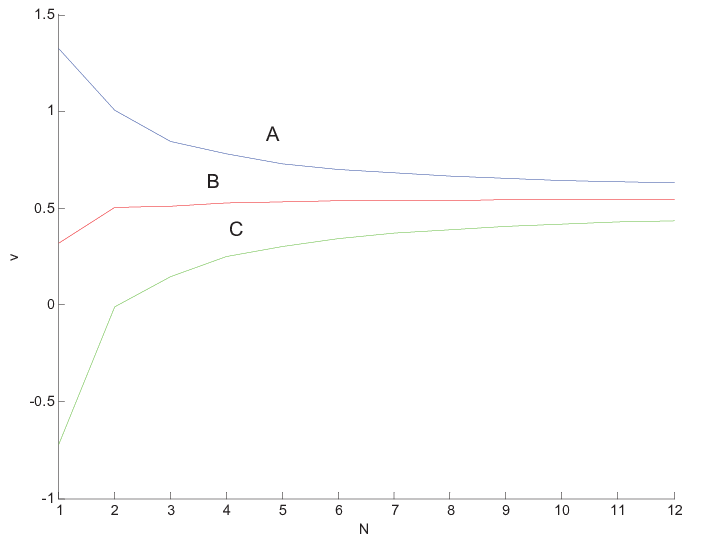
Note that (29) is calculated via Alg. 1 and s0=0s_{0}=0 due to the channel’s symmetry. However, calculating (30) is more difficult, since we have to maximize over all the probabilities r(xn||yn−1)r(x^{n}||y^{n-1}), and at the same time minimize over the initial state. Hence, we use another lower bound denoted by C¯∗\underline{C}^{*}, for which r(xn||yn−1)r(x^{n}||y^{n-1}) is fixed and is the one that achieves the maximum at (29), and we only minimize over s0s_{0}. Clearly, C¯∗≤C¯\underline{C}^{*}\leq\underline{C}. Fig. 4 presents the capacity estimation, and the upper and lower bound, as a function of the block length nn.

Refer to caption

Fig. 4: Plot of C¯n,Cn,C¯n∗\overline{C}_{n},\ C_{n},\ \underline{C}^{*}_{n} and the true capacity of the trapdoor channel with 2 states and feedback with delay 1.

In [21], the capacity of the trapdoor channel is calculated analytically, and given by

C=limn→∞Cn=log⁡(1+52)≈0.69424191.\displaystyle C=\lim_{n\rightarrow\infty}C_{n}=\log\left(\frac{1+\sqrt{5}}{2}\right)\approx 0.69424191. (31)

We see from the simulation that the upper and lower bounds of the capacity approach the limit in (31), and the estimated capacity at block length n=12n=12 is C12=0.6706533C_{12}=0.6706533.

V-B2 Directed information rate as a different estimator for the capacity

We now consider an estimator to the feedback capacity of an FSC by calculating (n+1)​Cn+1−n​Cn(n+1)C_{n+1}-nC_{n}. The justification for this estimator is based on the following lemma.

Lemma 6

. If limn→∞I⁡(Xn;Yn|Yn−1)\lim_{n\rightarrow\infty}I(X^{n};Y_{n}|Y^{n-1}) exists, then

limn→∞1n​I​(Xn→Yn)=limn→∞(I⁡(Xn→Yn)−I⁡(Xn−1→Yn−1)),\displaystyle\lim_{n\rightarrow\infty}\frac{1}{n}I(X^{n}\rightarrow Y^{n})=\lim_{n\rightarrow\infty}\left(I(X^{n}\rightarrow Y^{n})-I(X^{n-1}\rightarrow Y^{n-1})\right),

i.e.,

limn→∞Cn=limn→∞(n+1)​Cn+1−n​Cn.\displaystyle\lim_{n\rightarrow\infty}C_{n}=\lim_{n\rightarrow\infty}(n+1)C_{n+1}-nC_{n}.
Proof.

If we suppose that the limit above exists, then

limn→∞(I⁡(Xn→Yn)−I⁡(Xn−1→Yn−1))\displaystyle\lim_{n\rightarrow\infty}\left(I(X^{n}\rightarrow Y^{n})-I(X^{n-1}\rightarrow Y^{n-1})\right) =limn→∞I⁡(Xn;Yn|Yn−1)\displaystyle=\lim_{n\rightarrow\infty}I(X^{n};Y_{n}|Y^{n-1})
=(a)limn→∞1n​∑i=1nI⁡(Xi;Yi|Yi−1)\displaystyle\stackrel{{\scriptstyle(a)}}{{=}}\lim_{n\rightarrow\infty}\frac{1}{n}\sum_{i=1}^{n}I(X^{i};Y_{i}|Y^{i-1})
=limn→∞1n​I​(Xn→Yn),\displaystyle=\lim_{n\rightarrow\infty}\frac{1}{n}I(X^{n}\rightarrow Y^{n}),

where (a) follows from the fact that if the limit of the sequence {an}\{a_{n}\} exists, then the average of the sequence converges to the same limit. Further, a result from [7] provides that if the joint process {Xi,Yi}\{X_{i},Y_{i}\} is stationary, then the limit limn→∞I⁡(Xn;Yn|Yn−1)\lim_{n\rightarrow\infty}I(X^{n};Y_{n}|Y^{n-1}) exists. ∎

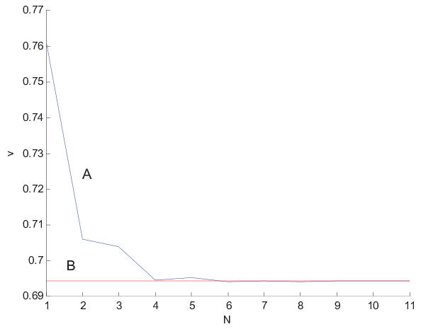
Fig. 5 presents the directed information rate estimator using the lemma above, and its comparison to the true capacity.
Refer to caption

Fig. 5: The upper line is (n+1)​Cn+1−n​Cn(n+1)C_{n+1}-nC_{n} calculated using Alg. 1 and the horizontal line is the analytical calculation, for the trapdoor channel with 2 states and feedback with delay 1.

One can see that the convergence of (n+1)​Cn+1−n​Cn(n+1)C_{n+1}-nC_{n} is faster than CnC_{n} and the upper and lower bounds as seen in Fig. 4, and achieves the value 0.69422850.6942285 when we calculate the 11t​h11^{th} difference. Furthermore, the convergence of the directed information rate stabilizes faster.

V-B3 M-State Trapdoor channel

We generalize the trapdoor channel to an M-state one.

Refer to caption

Fig. 6: Trapdoor channel with M states.

In the previous example we had M=2M=2 cells in the box, one for the state bit, and one for the input bit. One can consider the state to be the number of ’1’s in the channel before a new input is inserted. We can expand this notation, by letting the ’box’ contain more than 2 cells as presented in Fig. 6. Here, the state at any given time will express the number of 1′1^{\prime}s that are in the box at that time, and each cell has even probability to be chosen for the output. In this case, MM cells in the box are equivalent to MM states of the channel. By that definition we can see that the state si−1s_{i-1} as a function of past input, output, and the initial state is given by

si−1\displaystyle s_{i-1} =\displaystyle= xi−1+si−2−yi−1\displaystyle x_{i-1}+s_{i-2}-y_{i-1}
=\displaystyle= s0+∑j=1i−1(xj−yj).\displaystyle s_{0}+\sum_{j=1}^{i-1}(x_{j}-y_{j}).

Moreover, for calculating the channel probability p⁡(yi=1|xi,yi−1,s0)p(y_{i}=1|x^{i},y^{i-1},s_{0}), we add si−1s_{i-1} to xix_{i} and divide the sum by the number of cells, i.e.,

p⁡(yi=1|xi,yi−1,s0)=si−1+xim.\displaystyle p(y_{i}=1|x^{i},y^{i-1},s_{0})=\frac{s_{i-1}+x_{i}}{m}.

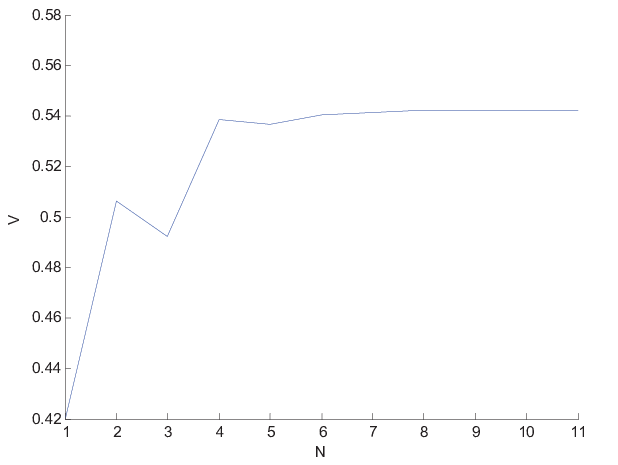
Now that we have p(yn||xn,s0)p(y^{n}||x^{n},s_{0}), we use Alg. 1 for calculating CnC_{n} for every n∈{1,2,…,12}n\in\{1,2,...,12\}. Fig. 7 presents the directed information rate estimator (n+1)​Cn+1−n​Cn(n+1)C_{n+1}-nC_{n} for the trapdoor channel with M=3M=3 cells.

Refer to caption

Fig. 7: Plot of (n+1)​Cn+1−n​Cn(n+1)C_{n+1}-nC_{n} for the trap door channel with 3 cells and feedback with delay 1.

Note, that in Fig. 7 we achieve the value 0.54239840.5423984 in the 11t​h11^{th} difference, thus we can assume that the capacity of a 3-state trapdoor channel is approximately 0.5420.542.

V-B4 Influence of the number of cells on the capacity

To summarize the trapdoor channel example, we examine the way the number of cells affects the capacity.

Refer to caption

Fig. 8: Change of 12​C12−11​C1112C_{12}-11C_{11} over the number of cells in the trapdoor channel with feedback with delay 1.

The estimation use is the directed information rate, with n=12n=12. In Fig. 8 we can see that the capacity decreases as the number of cells increases and approaches zero.

V-C The Ising channel

The Ising model is a mathematical model of ferromagnetism in statistical mechanics. It was originally proposed by the physicist Wilhelm Lenz who gave it as a problem to his student Ernst Ising after whom it is named. The model consists of discrete variables called spins that can be in one of two states. The spins are arranged in a lattice or graph, and each spin interacts only with its nearest neighbors.

The Ising channel is based on its physical model, and simulates Intersymbol Interference where the state of the channel at time ii is the current input, and the output is determined by the input at time i+1i+1.

Refer to caption

Fig. 9: The Ising Channel.[30]

The channel (without feedback) was introduced by Berger and Bonomi [30] and is depicted in Fig. 9. In their paper, they proved the existence of bounds for the no-feedback case. In addition, they showed that the zero-error capacity without feedback is 0.50.5.

V-C1 Ising channel with delay d=2d=2

We estimate the capacity of the Ising channel with feedback.
Refer to caption
(a)

Refer to caption
(b)
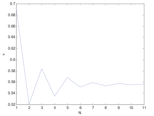
Fig. 10: Performance of Alg. 1 on the Ising channel with feedback delay of d=2d=2. In (a) we present C¯n,Cn,C¯n∗\overline{C}_{n},\ C_{n},\ \underline{C}^{*}_{n}, and in (b) we have (n+1)​Cn+1−n​Cn(n+1)C_{n+1}-nC_{n}.

Since the output at time ii is determined by the input at times i,i+1i,\ i+1, we define the channel PMF as p(y0n−1||xn,s0)p(y_{0}^{n-1}||x^{n},s_{0}). Therefore, the feedback at time ii must be the output at time i−2i-2, since we cannot have yi−1y_{i-1} before xi−1x_{i-1} is sent. Thus, looking at the Ising channel with delay d=1d=1 is not a practical example, and we did not examine it. We ran our algorithm on the Ising channel, with delayed feedback of d=2d=2; the results are presented in Fig. 10. In Fig. 10 (a), we obtain C12=0.5459C_{12}=0.5459, and in (b) we achieve 12​C12−11​C11=0.556312C_{12}-11C_{11}=0.5563 in the 11t​h11^{th} difference.

V-C2 The effects the delay has on the capacity

Here we investigate how the delay influences the capacity. We do so by computing the directed information rate estimator of the Ising channel with blocks of length 1212, over the feedback delay d={2,3,…,12}d=\{2,3,...,12\}. The formulas for estimating the capacity when the delay is bigger than 1 is given in Section III, equations (14), (15). In Fig. 11 we can see that, as expected, the capacity decreases as the delay increases. This is due to the fact that we have less knowledge of the output to use.

Refer to caption

Fig. 11: Change of 12​C12−11​C1112C_{12}-11C_{11} over the delay of the feedback on the Ising channel.

VI CONCLUSIONS

In this paper, we generalized the classical BAA for maximizing the directed information over causal conditioning, i.e., calculating

Cn=1nmaxp(xn||yn−1)I(Xn→Yn).\displaystyle C_{n}=\frac{1}{n}\max_{p(x^{n}||y^{n-1})}I(X^{n}\rightarrow Y^{n}).

The optimizing the directed information is necessary for estimating the capacity of an FSC with feedback. As we attempted to solve this problem we found that difficulties arose regarding the causal conditioning probability we tried to optimize over. We overcame this barrier by using an additional backwards loop to find all components of the causal conditioned probability, separately.

Another application of optimizing the directed information is to estimate the rate distortion function for source coding with feed forward as presented in [31], [32], [33]. In our future work [34], we address the source coding with feedforward problem, and derive bounds for stationary and ergodic sources. We also present and prove a BA-type algorithm for obtaining a numerical solution that computes these bounds.

Appendix A General case for channel coding-Feedback that is a function of the delayed output

Here we extend Alg. 1, given in Section IV, for channels where the encoder has specific information about the delayed output. In this case, the input probability is given by r(xn||zn−d)r(x^{n}||z^{n-d}), where zi=f⁡(yi)z_{i}=f(y_{i}) is the feedback, and ff is deterministic. In other words, we solve the optimization problem given by

maxr(xn||zn−d)I(Xn→Yn).\displaystyle\max_{r(x^{n}||z^{n-d})}I(X^{n}\rightarrow Y^{n}).

The optimization problem is associated to Fig. 12.

Refer to caption

Fig. 12: Channel with delayed feedback as a function of the output.

The proof for this case is similar to that of Theorem 1, except the steps that follow from Lemmas 4 and 5. Lemma 4 proves the existence of an argument q⁡(xn|yn)q(x^{n}|y^{n}) that maximizes the directed information where r(xn||yn−1)r(x^{n}||y^{n-1}) is fixed. The modification of this lemma is presented here, where we find the argument q⁡(xn|yn)q(x^{n}|y^{n}) that maximizes the directed information where r(xn||zn−d)r(x^{n}||z^{n-d}) is fixed; the proof is omitted. Therefore, the maximization over q⁡(xn|yn)q(x^{n}|y^{n}) where r(xn||zn−d)r(x^{n}||z^{n-d}) is fixed is given by

q∗​(xn|yn)=r(xn||zn−d)p(yn||xn)∑xnr(xn||zn−d)p(yn||xn).\displaystyle q^{*}(x^{n}|y^{n})=\frac{r(x^{n}||z^{n-d})p(y^{n}||x^{n})}{\sum_{x^{n}}{r(x^{n}||z^{n-d})p(y^{n}||x^{n})}}.

Lemma 5 proves the existence of an argument r(xn||yn−1)r(x^{n}||y^{n-1}) that maximizes the directed information where q⁡(xn|yn)q(x^{n}|y^{n}) is fixed. We replace this lemma by Lemma 7.

Lemma 7

. For fixed q⁡(xn|yn)q(x^{n}|y^{n}), there exists c1​(q)c_{1}(q) that achieves maxr(xn||zn−d)I(Xn→Yn),\max_{r(x^{n}||z^{n-d})}I(X^{n}\rightarrow Y^{n}), and given by

r(xn||zn−d)=∏i=1nr(xi|xi−1,zi−d),\displaystyle r(x^{n}||z^{n-d})=\prod_{i=1}^{n}{r(x_{i}|x^{i-1},z^{i-d})},

where

r⁡(xi|xi−1,zi−d)=r′​(xi,zi−d)∑xir′​(xi,zi−d),r(x_{i}|x^{i-1},z^{i-d})=\frac{r^{\prime}(x^{i},z^{i-d})}{\sum_{x^{i}}r^{\prime}(x^{i},z^{i-d})}, (32)

and

r′​(xi,zi−d)=∏xi+1n,yi−d+1n∏Ai,d,z[q⁡(xn|yn)∏j=i+1nr⁡(xj|xj−1,zj−d)]p(yn||xn)∏j=i+1nr(xj|xj−1,zj−d)∑Ai,d,z∏j=1i−dp⁡(yj|xj,yj−1).\displaystyle r^{\prime}(x^{i},z^{i-d})=\prod_{x_{i+1}^{n},y_{i-d+1}^{n}}\prod_{A_{i,d,z}}{\left[\frac{q(x^{n}|y^{n})}{\prod_{j=i+1}^{n}{r(x_{j}|x^{j-1},z^{j-d})}}\right]^{\frac{p(y^{n}||x^{n})\prod_{j=i+1}^{n}{r(x_{j}|x^{j-1},z^{j-d})}}{\sum_{A_{i,d,z}}\prod_{j=1}^{i-d}{p(y_{j}|x^{j},y^{j-1})}}}}. (33)
Proof.

We find the products of r(xn||zn−d)r(x^{n}||z^{n-d}) that achieve maximum for the directed information. For convenience, let us use for short: ri≜r⁡(xi|xi−1,zi−d)r_{i}\triangleq r(x_{i}|x^{i-1},z^{i-d}), and pi≜p⁡(yi|xi,yi−1)p_{i}\triangleq p(y_{i}|x^{i},y^{i-1}). As in Lemma 2 we can omit that I⁡(Xn→Yn)I(X^{n}\rightarrow Y^{n}) is concave in {r(xn||yn−d),q(xn|yn)}\{r(x^{n}||y^{n-d}),\ q(x^{n}|y^{n})\}. Furthermore, the constraints of the optimization problem are affine, and we can use the Lagrange multipliers method with the Karush-Kuhn-Tucker conditions. We define the Lagrangian as:

J=∑xn,yn(p(yn||xn)∏i=1nrilog(q⁡(xn|yn)∏j=1nrj))+∑i=1n(∑xi−1,zi−dνi,(xi−1,zi−d)(∑xiri−1)).\displaystyle J=\sum_{x^{n},y^{n}}{\left(p(y^{n}||x^{n})\prod_{i=1}^{n}{r_{i}}\log\left(\frac{q(x^{n}|y^{n})}{\prod_{j=1}^{n}{r_{j}}}\right)\right)}+\sum_{i=1}^{n}{\left(\sum_{x^{i-1},z^{i-d}}\nu_{i,(x^{i-1},z^{i-d})}\left(\sum_{x_{i}}{r_{i}}-1\right)\right)}.

Now, for every i∈{1..n}i\in\{1..n\} we find rir_{i} s.t.,

∂J∂ri\displaystyle\frac{\partial J}{\partial r_{i}} =∑xi+1n,yi−d+1n,Ai,d,z(p(yn||xn)∏j≠i=1nrj[logq⁡(xn|yn)∏j=1nrj−1])+νi,(xi−1,zi−d)\displaystyle=\sum_{x_{i+1}^{n},y_{i-d+1}^{n},A_{i,d,z}}{\left(p(y^{n}||x^{n})\prod_{j\neq i=1}^{n}{r_{j}}\left[\log{\frac{q(x^{n}|y^{n})}{\prod_{j=1}^{n}{r_{j}}}}-1\right]\right)}+\nu_{i,(x^{i-1},z^{i-d})}
=∑Ai,d,z∏j=1i−1rj∑xi+1n,yi−d+1n(p(yn||xn)∏j=i+1nrj[logq⁡(xn|yn)∏j=i+1nrj−log∏j=1i−1rj−logri−1])+νi,(xi−1,zi−d)\displaystyle=\sum_{A_{i,d,z}}\prod_{j=1}^{i-1}{r_{j}}\sum_{x_{i+1}^{n},y_{i-d+1}^{n}}{\left(p(y^{n}||x^{n})\prod_{j=i+1}^{n}{r_{j}}\left[\log{\frac{q(x^{n}|y^{n})}{\prod_{j=i+1}^{n}{r_{j}}}}-\log{\prod_{j=1}^{i-1}{r_{j}}}-\log{r_{i}}-1\right]\right)}+\nu_{i,(x^{i-1},z^{i-d})}
=0,\displaystyle=0,

where the set Ai,d,z={yi−d:zi−d=f⁡(yi−d)}A_{i,d,z}=\{y^{i-d}:z^{i-d}=f(y^{i-d})\} stands for all output sequences yi−dy^{i-d} s.t. the function in the delay maps them to the same sequence zi−dz^{i-d}, which is the feedback.

Note that since ∏j=1i−1rj\prod_{j=1}^{i-1}{r_{j}} does not depend on Ai,d,zA_{i,d,z}, we can take the product out of the sum. Furthermore, since νi\nu_{i} is a function of (xi−1,zi−d)(x^{i-1},z^{i-d}) we can divide the whole equation by the product above, and get a new νi,(xi−1,zi−d)∗\nu^{*}_{i,(x^{i-1},z^{i-d})}. Moreover, we can see that three of the expressions in the sum, i.e., {log∏j=1i−1rj,logri, 1}\{\log{\prod_{j=1}^{i-1}{r_{j}}},\ \log{r_{i}},\ 1\}, do not depend on (xi+1n,yi−d+1n)(x_{i+1}^{n},y_{i-d+1}^{n}), thus leaving their coefficient in the equation to be

∑xi+1n,yi−d+1n,Ai,d,zp(yn||xn)∏j=i+1nrj=∑Ai,d,z∏j=1i−dpj.\displaystyle\sum_{x_{i+1}^{n},y_{i-d+1}^{n},A_{i,d,z}}{p(y^{n}||x^{n})\prod_{j=i+1}^{n}{r_{j}}}=\sum_{A_{i,d,z}}\prod_{j=1}^{i-d}{p_{j}}.

Hence we obtain:

log⁡[∏xi+1n,yi−d+1n(q⁡(xn|yn)∏j=i+1nrj)p(yn||xn)∏j=i+1nrj∑Ai,d,z∏j=1i−dpj]−log⁡ri−log⁡νi,(xi−1,zi−d)∗⁣∗=0,\displaystyle\log\left[\prod_{x_{i+1}^{n},y_{i-d+1}^{n}}{\left(\frac{q(x^{n}|y^{n})}{\prod_{j=i+1}^{n}{r_{j}}}\right)^{\frac{p(y^{n}||x^{n})\prod_{j=i+1}^{n}{r_{j}}}{\sum_{A_{i,d,z}}{\prod_{j=1}^{i-d}{p_{j}}}}}}\right]-\log{r_{i}}-\log\nu^{**}_{i,(x^{i-1},z^{i-d})}=0,

where

logνi,(xi−1,zi−d)∗⁣∗=∑Ai,d,z∏j=1i−dpj(1+log∏j=1i−1rj)−νi,(xi−1,zi−d)∗.\log{\nu^{**}_{i,(x^{i-1},z^{i-d})}}=\sum_{A_{i,d,z}}{\prod_{j=1}^{i-d}{p_{j}}}\left(1+\log{\prod_{j=1}^{i-1}{r_{j}}}\right)-\nu^{*}_{i,(x^{i-1},z^{i-d})}.

Therefore, we are left with the expression:

r⁡(xi|xi−1,zi−d)=r′​(xi,zi−d)∑xir′​(xi,zi−d),r(x_{i}|x^{i-1},z^{i-d})=\frac{r^{\prime}(x^{i},z^{i-d})}{\sum_{x^{i}}r^{\prime}(x^{i},z^{i-d})},

where

r′​(xi,zi−d)=∏xi+1n,yi−d+1n,Ai,d,z[q⁡(xn|yn)∏j=i+1nr⁡(xj|xj−1,zj−d)]p(yn||xn)∏j=i+1nr(xj|xj−1,zj−d)∑Ai,d,z∏j=1i−dp⁡(yj|xj,yj−1).\displaystyle r^{\prime}(x^{i},z^{i-d})=\prod_{x_{i+1}^{n},y_{i-d+1}^{n},A_{i,d,z}}{\left[\frac{q(x^{n}|y^{n})}{\prod_{j=i+1}^{n}{r(x_{j}|x^{j-1},z^{j-d})}}\right]^{\frac{p(y^{n}||x^{n})\prod_{j=i+1}^{n}{r(x_{j}|x^{j-1},z^{j-d})}}{\sum_{A_{i,d,z}}\prod_{j=1}^{i-d}{p(y_{j}|x^{j},y^{j-1})}}}}. (34)

As in Section IV, we can see that for all ii, rir_{i} is dependent on q⁡(xn|yn)q(x^{n}|y^{n}) and {ri+1,ri+2,…,rn}\{r_{i+1},r_{i+2},...,r_{n}\}, and rnr_{n} is a function of q⁡(xn|yn)q(x^{n}|y^{n}) alone. Thus, we use the Backwards maximization method. After calculating rir_{i} for all i=1,…,ni={1,...,n}, we obtain r(xn||zn−d)=∏i=1nrir(x^{n}||z^{n-d})=\prod_{i=1}^{n}{r_{i}} that maximizes the directed information where q⁡(xn|yn)q(x^{n}|y^{n}) is fixed, i.e., c1​(q)c_{1}(q) and the lemma is proven. ∎

As mentioned, by replacing Lemmas 4, 5 by those given here, we can follow the outline of Theorem 1 and conclude the existence of an alternating maximization procedure, i.e., we can compute

Cn=1nmaxr(xn||zn−d)I(Xn→Yn)\displaystyle C_{n}=\frac{1}{n}\max_{r(x^{n}||z^{n-d})}I(X^{n}\rightarrow Y^{n})

that is equal to limk→∞IL​(k)\lim_{k\rightarrow\infty}I_{L}(k), where IL​(k)I_{L}(k) is the value of ILI_{L} in the kkth iteration in the extended algorithm. One more step is required in order to prove the extension of Alg. 1 to the case presented here; the existence of IUI_{U}. This part is presented in Appendix B.

Appendix B Proof of Theorem 2

Here, we prove the existence of an upper bound, IUI_{U}, that converges to CnC_{n} from above simultaneously with the convergence on ILI_{L} to it from below, as in Alg. 1. To this purpose, we present and prove few lemmas that assist in obtaining our main goal. We start with Lemma 8 that gives an inequality for the directed information. This inequality is used in Lemma 9 to prove the existence of our upper bound which Lemma 10 proves to be tight. Theorem 2 combines Lemmas 9, 10.

Lemma 8

. Let Ir1​(Xn→Yn)I_{r_{1}}(X^{n}\rightarrow Y^{n}) correspond to r1(xn||yn−d)r_{1}(x^{n}||y^{n-d}), then for every r0(xn||yn−d)r_{0}(x^{n}||y^{n-d}),

Ir1(Xn→Yn)≤∑xn,yn−dr1(xn||yn−d)∑yn−d+1np(yn||xn)logp(yn||xn)∑x′np(yn||x′n)⋅r0(x′n||yn−d).\displaystyle I_{r_{1}}(X^{n}\rightarrow Y^{n})\leq\sum_{x^{n},y^{n-d}}r_{1}(x^{n}||y^{n-d})\sum_{y_{n-d+1}^{n}}p(y^{n}||x^{n})\log\frac{p(y^{n}||x^{n})}{\sum_{x^{\prime n}}p(y^{n}||x^{\prime n})\cdot r_{0}(x^{\prime n}||y^{n-d})}.
Proof.

For any r1(xn||yn−d)r_{1}(x^{n}||y^{n-d}), r0(xn||yn−d)r_{0}(x^{n}||y^{n-d}),

∑xn,yn−dr1(xn||yn−d)\displaystyle\sum_{x^{n},y^{n-d}}r_{1}(x^{n}||y^{n-d}) ∑yn−d+1np(yn||xn)logp(yn||xn)∑x′np(yn||x′n)⋅r0(x′n||yn−d)−Ir1(Xn→Yn)\displaystyle\sum_{y_{n-d+1}^{n}}p(y^{n}||x^{n})\log\frac{p(y^{n}||x^{n})}{\sum_{x^{\prime n}}p(y^{n}||x^{\prime n})\cdot r_{0}(x^{\prime n}||y^{n-d})}-I_{r_{1}}(X^{n}\rightarrow Y^{n})
=∑xn,ynr1(xn||yn−d)⋅p(yn||xn)logp(yn||xn)∑x′np(yn||x′n)⋅r0(x′n||yn−d)\displaystyle=\sum_{x^{n},y^{n}}r_{1}(x^{n}||y^{n-d})\cdot p(y^{n}||x^{n})\log{\frac{p(y^{n}||x^{n})}{\sum_{{x^{\prime}}^{n}}p(y^{n}||x^{\prime n})\cdot r_{0}(x^{\prime n}||y^{n-d})}}
−∑xn,ynr1(xn||yn−d)⋅p(yn||xn)logp(yn||xn)∑x′np(yn||x′n)⋅r1(x′n||yn−d)\displaystyle\ \ \ -\sum_{x^{n},y^{n}}r_{1}(x^{n}||y^{n-d})\cdot p(y^{n}||x^{n})\log{\frac{p(y^{n}||x^{n})}{\sum_{{x^{\prime}}^{n}}p(y^{n}||x^{\prime n})\cdot r_{1}(x^{\prime n}||y^{n-d})}}
=∑xn,ynr1(xn||yn−d)⋅p(yn||xn)log∑x′np(yn||x′n)⋅r1(x′n||yn−d)∑x′np(yn||x′n)⋅r0(x′n||yn−d)\displaystyle=\sum_{x^{n},y^{n}}r_{1}(x^{n}||y^{n-d})\cdot p(y^{n}||x^{n})\log{\frac{\sum_{{x^{\prime}}^{n}}p(y^{n}||x^{\prime n})\cdot r_{1}(x^{\prime n}||y^{n-d})}{\sum_{{x^{\prime}}^{n}}p(y^{n}||x^{\prime n})\cdot r_{0}(x^{\prime n}||y^{n-d})}}
=∑ynp1​(yn)​log⁡p1​(yn)p0​(yn)\displaystyle=\sum_{y^{n}}p_{1}(y^{n})\log{\frac{p_{1}(y^{n})}{p_{0}(y^{n})}}
=(a)D(p1(yn)||p0(yn))\displaystyle\stackrel{{\scriptstyle(a)}}{{=}}D\left(p_{1}(y^{n})||p_{0}(y^{n})\right)
≥(b)0,\displaystyle\stackrel{{\scriptstyle(b)}}{{\geq}}0,

where in (a), p0​(yn)p_{0}(y^{n}) and p1​(yn)p_{1}(y^{n}) are the PMFs of yny^{n} that corresponds to r0(x′n||yn−d)r_{0}(x^{\prime n}||y^{n-d}) and r1(x′n||yn−d)r_{1}(x^{\prime n}||y^{n-d}), and (b) follows from the non negativity of the divergence. Thus, the lemma is proven. ∎

Our next lemma uses the inequality in Lemma 8 to show the existence of the upper bound, which is the first step in proving Theorem 2.

Lemma 9

. For every r0(xn||yn−d)r_{0}(x^{n}||y^{n-d}),

Cn≤IU,\displaystyle C_{n}\leq I_{U},

where

IU=1nmaxxd∑y1maxxd+1∑y2⋯maxxn∑yn−d+1np(yn||xn)logp(yn||xn)∑x′np(yn||x′n)⋅r0(x′n||yn−d).\displaystyle I_{U}=\frac{1}{n}\max_{x^{d}}\sum_{y_{1}}\max_{x_{d+1}}\sum_{y_{2}}\cdots\max_{x_{n}}\sum_{y_{n-d+1}^{n}}p(y^{n}||x^{n})\log\frac{p(y^{n}||x^{n})}{\sum_{x^{\prime n}}p(y^{n}||x^{\prime n})\cdot r_{0}(x^{\prime n}||y^{n-d})}.
Proof.

To prove this lemma, we first use lemma 8. For every r1(xn||yn−d),r0(xn||yn−d)r_{1}(x^{n}||y^{n-d}),\ r_{0}(x^{n}||y^{n-d}),

Ir1​(Xn→Yn)\displaystyle I_{r_{1}}(X^{n}\rightarrow Y^{n}) ≤(a)∑xn,yn−dr1(xn||yn−d)∑yn−d+1np(yn||xn)logp(yn||xn)∑x′np(yn||x′n)⋅r0(x′n||yn−d)\displaystyle\stackrel{{\scriptstyle(a)}}{{\leq}}\sum_{x^{n},y^{n-d}}r_{1}(x^{n}||y^{n-d})\sum_{y_{n-d+1}^{n}}p(y^{n}||x^{n})\log\frac{p(y^{n}||x^{n})}{\sum_{x^{\prime n}}p(y^{n}||x^{\prime n})\cdot r_{0}(x^{\prime n}||y^{n-d})}
≤(b)∑xn,yn−d∏i=1nr1​(xi|xi−1,yi−d)​maxxn∑yn−d+1np(yn||xn)logp(yn||xn)∑x′np(yn||x′n)⋅r0(x′n||yn−d)⏟f⁡(xn−1,yn−d)\displaystyle\stackrel{{\scriptstyle(b)}}{{\leq}}\sum_{x^{n},y^{n-d}}\prod_{i=1}^{n}r_{1}(x_{i}|x^{i-1},y^{i-d})\underbrace{\max_{x_{n}}\sum_{y_{n-d+1}^{n}}p(y^{n}||x^{n})\log\frac{p(y^{n}||x^{n})}{\sum_{x^{\prime n}}p(y^{n}||x^{\prime n})\cdot r_{0}(x^{\prime n}||y^{n-d})}}_{\textrm{$f(x^{n-1},y^{n-d})$}}
=(c)∑xn−1,yn−d−1∏i=1n−1r1​(xi|xi−1,yi−d)​∑yn−dmaxxn∑yn−d+1np(yn||xn)logp(yn||xn)∑x′np(yn||x′n)⋅r0(x′n||yn−d)⏟f⁡(xn−1,yn−d−1)\displaystyle\stackrel{{\scriptstyle(c)}}{{=}}\sum_{x^{n-1},y^{n-d-1}}\prod_{i=1}^{n-1}r_{1}(x_{i}|x^{i-1},y^{i-d})\underbrace{\sum_{y_{n-d}}\max_{x_{n}}\sum_{y_{n-d+1}^{n}}p(y^{n}||x^{n})\log\frac{p(y^{n}||x^{n})}{\sum_{x^{\prime n}}p(y^{n}||x^{\prime n})\cdot r_{0}(x^{\prime n}||y^{n-d})}}_{\textrm{$f(x^{n-1},y^{n-d-1})$}}
≤∑xn−1,yn−d−1∏i=1n−1r1​(xi|xi−1,yi−d)​maxxn−1∑yn−dmaxxn∑yn−d+1np(yn||xn)logp(yn||xn)∑x′np(yn||x′n)⋅r0(x′n||yn−d)⏟f⁡(xn−2,yn−d−1)\displaystyle\leq\sum_{x^{n-1},y^{n-d-1}}\prod_{i=1}^{n-1}r_{1}(x_{i}|x^{i-1},y^{i-d})\underbrace{\max_{x_{n-1}}\sum_{y_{n-d}}\max_{x_{n}}\sum_{y_{n-d+1}^{n}}p(y^{n}||x^{n})\log\frac{p(y^{n}||x^{n})}{\sum_{x^{\prime n}}p(y^{n}||x^{\prime n})\cdot r_{0}(x^{\prime n}||y^{n-d})}}_{\textrm{$f(x^{n-2},y^{n-d-1})$}}
≤∑xd∏i=1dr1​(xi|xi−1,yi−d)​∑y1maxxd+1∑y2⋯maxxn∑yn−d+1np(yn||xn)logp(yn||xn)∑x′np(yn||x′n)⋅r0(x′n||yn−d)⏟f⁡(xd)\displaystyle\leq\sum_{x^{d}}\prod_{i=1}^{d}r_{1}(x_{i}|x^{i-1},y^{i-d})\underbrace{\sum_{y_{1}}\max_{x_{d+1}}\sum_{y_{2}}\cdots\max_{x_{n}}\sum_{y_{n-d+1}^{n}}p(y^{n}||x^{n})\log\frac{p(y^{n}||x^{n})}{\sum_{x^{\prime n}}p(y^{n}||x^{\prime n})\cdot r_{0}(x^{\prime n}||y^{n-d})}}_{\textrm{$f(x^{d})$}}
≤∑xd∏i=1dr1​(xi|xi−1,yi−d)⏟=1​maxxd∑y1maxxd+1∑y2⋯maxxn∑yn−d+1np(yn||xn)logp(yn||xn)∑x′np(yn||x′n)⋅r0(x′n||yn−d)⏟∈ℝ\displaystyle\leq\underbrace{\sum_{x^{d}}\prod_{i=1}^{d}r_{1}(x_{i}|x^{i-1},y^{i-d})}_{\textrm{$=1$}}\underbrace{\max_{x^{d}}\sum_{y_{1}}\max_{x_{d+1}}\sum_{y_{2}}\cdots\max_{x_{n}}\sum_{y_{n-d+1}^{n}}p(y^{n}||x^{n})\log\frac{p(y^{n}||x^{n})}{\sum_{x^{\prime n}}p(y^{n}||x^{\prime n})\cdot r_{0}(x^{\prime n}||y^{n-d})}}_{\textrm{$\in\mathbb{R}$}}
=maxxd∑y1maxxd+1∑y2⋯maxxn∑yn−d+1np(yn||xn)logp(yn||xn)∑x′np(yn||x′n)⋅r0(x′n||yn−d),\displaystyle=\max_{x^{d}}\sum_{y_{1}}\max_{x_{d+1}}\sum_{y_{2}}\cdots\max_{x_{n}}\sum_{y_{n-d+1}^{n}}p(y^{n}||x^{n})\log\frac{p(y^{n}||x^{n})}{\sum_{x^{\prime n}}p(y^{n}||x^{\prime n})\cdot r_{0}(x^{\prime n}||y^{n-d})},

where (a) follows Lemma 8, (b) follows from maximizing an expression over xnx_{n}, and (c) follows from the fact that the expression in the under-brace is a function of xn−1,yn−dx^{n-1},y^{n-d}, and we can take it out of the summation over xnx_{n} and use ∑xnr⁡(xn|xn−1,yn−d)=1\sum_{x_{n}}r(x_{n}|x^{n-1},y^{n-d})=1. The rest of the steps are the same as (b) and (c), where we refer to a different xix_{i}.

Since the inequality above is true for every r1(xn||yn−d)r_{1}(x^{n}||y^{n-d}), we can use it on rc(xn||yn−d)r_{c}(x^{n}||y^{n-d}) that achieves CnC_{n}, and thus for every r0(xn||yn−d)r_{0}(x^{n}||y^{n-d})

Cn≤1nmaxxd∑y1maxxd+1∑y2⋯maxxn∑yn−d+1np(yn||xn)logp(yn||xn)∑x′np(yn||x′n)⋅r0(x′n||yn−d).\displaystyle C_{n}\leq\frac{1}{n}\max_{x^{d}}\sum_{y_{1}}\max_{x_{d+1}}\sum_{y_{2}}\cdots\max_{x_{n}}\sum_{y_{n-d+1}^{n}}p(y^{n}||x^{n})\log\frac{p(y^{n}||x^{n})}{\sum_{x^{\prime n}}p(y^{n}||x^{\prime n})\cdot r_{0}(x^{\prime n}||y^{n-d})}.

This is also true for every r0(xn||yn−d)r_{0}(x^{n}||y^{n-d}), and hence for the minimum over all r0(xn||yn−d)r_{0}(x^{n}||y^{n-d}), and we obtain

Cn≤1nminr0maxxd∑y1maxxd+1∑y2⋯maxxn∑yn−d+1np(yn||xn)logp(yn||xn)∑x′np(yn||x′n)⋅r0(x′n||yn−d),\displaystyle C_{n}\leq\frac{1}{n}\min_{r_{0}}\max_{x^{d}}\sum_{y_{1}}\max_{x_{d+1}}\sum_{y_{2}}\cdots\max_{x_{n}}\sum_{y_{n-d+1}^{n}}p(y^{n}||x^{n})\log\frac{p(y^{n}||x^{n})}{\sum_{x^{\prime n}}p(y^{n}||x^{\prime n})\cdot r_{0}(x^{\prime n}||y^{n-d})},

and the lemma is proven. ∎

The next part of Theorem 2 is to show that the bound is tight.

Lemma 10

. The upper bound in Lemma 9 is tight, and is obtained by r(xn||yn−d)r(x^{n}||y^{n-d}) that achieves the capacity.

Proof.

In Lemma 9, we showed only half of the proof of the theorem, i.e., the existence of an upper bound. To prove this lemma, we need to show that this inequality is tight. For that purpose, we use the Lagrange multipliers method with the KKT conditions with respect to all r⁡(xi|xi−1,yi−d)r(x_{i}|x^{i-1},y^{i-d})s. We can use the KKT conditions since the directed information is a concave function in all r⁡(xi|xi−1,yi−d)r(x_{i}|x^{i-1},y^{i-d})s, as seen in Lemma 3.

We define the Lagrangian as

J=∑xn,ynr(xn||yn−d)\displaystyle J=\sum_{x^{n},y^{n}}r(x^{n}||y^{n-d}) ⋅p(yn||xn)logp(yn||xn)∑x′np(yn||x′n)⋅r(x′n||yn−d)\displaystyle\cdot p(y^{n}||x^{n})\log{\frac{p(y^{n}||x^{n})}{\sum_{{x^{\prime}}^{n}}p(y^{n}||x^{\prime n})\cdot r(x^{\prime n}||y^{n-d})}}
−∑i=1n∑xi−1,yi−dνi,(xi−1,yi−d)(∑xir(xi|xi−1,yi−d)−1)+∑i=1n∑xi−1,yi−dhi,(xi−1,yi−d)r(xi|xi−1,yi−d).\displaystyle-\sum_{i=1}^{n}\sum_{x^{i-1},y^{i-d}}\nu_{i,(x^{i-1},y^{i-d})}(\sum_{x_{i}}r(x_{i}|x^{i-1},y^{i-d})-1)+\sum_{i=1}^{n}\sum_{x^{i-1},y^{i-d}}h_{i,(x^{i-1},y^{i-d})}r(x_{i}|x^{i-1},y^{i-d}).

Now, for every r⁡(xi|xi−1,yi−d)r(x_{i}|x^{i-1},y^{i-d}), we have

∂J∂r⁡(xi|xi−1,yi−d)\displaystyle\frac{\partial J}{\partial r(x_{i}|x^{i-1},y^{i-d})} =∑xi+1,yi−d+1r(xi+1|xi,yi−d+1)⋯∑xn,yn−dr(xn|xn−1,yn−d)⋅\displaystyle=\sum_{x_{i+1},y_{i-d+1}}r(x_{i+1}|x^{i},y^{i-d+1})\cdots\sum_{x_{n},y_{n-d}}r(x_{n}|x^{n-1},y^{n-d})\cdot
∑yn−d+1np(yn||xn)logp(yn||xn)∑x′np(yn||x′n)⋅r(x′n||yn−d)−νi,(xi−1,yi−d)+hi,(xi−1,yi−d).\displaystyle\ \ \ \ \ \ \sum_{y_{n-d+1}^{n}}p(y^{n}||x^{n})\log\frac{p(y^{n}||x^{n})}{\sum_{x^{\prime n}}p(y^{n}||x^{\prime n})\cdot r(x^{\prime n}||y^{n-d})}-\nu_{i,(x^{i-1},y^{i-d})}+h_{i,(x^{i-1},y^{i-d})}.

Setting ∂J∂r⁡(xi|xi−1,yi−d)=0\frac{\partial J}{\partial r(x_{i}|x^{i-1},y^{i-d})}=0 we are left with two cases. For r⁡(xi|xi−1,yi−d)>0r(x_{i}|x^{i-1},y^{i-d})>0 the KKT conditions requires us to set hi=0h_{i}=0 and we obtain

∑xi+1,yi−d+1r(xi+1|xi,yi−d+1)⋯∑xn,yn−dr(xn|xn−1,yn−d)∑yn−d+1np(yn||xn)logp(yn||xn)∑x′np(yn||x′n)⋅r(x′n||yn−d)=νi,\displaystyle\sum_{x_{i+1},y_{i-d+1}}r(x_{i+1}|x^{i},y^{i-d+1})\cdots\sum_{x_{n},y_{n-d}}r(x_{n}|x^{n-1},y^{n-d})\sum_{y_{n-d+1}^{n}}p(y^{n}||x^{n})\log\frac{p(y^{n}||x^{n})}{\sum_{x^{\prime n}}p(y^{n}||x^{\prime n})\cdot r(x^{\prime n}||y^{n-d})}=\nu_{i},

whereas for r⁡(xi|xi−1,yi−d)=0r(x_{i}|x^{i-1},y^{i-d})=0 we set hi>0h_{i}>0 and the equality becomes an inequality.

We now analyze our results for the case where r⁡(xi|xi−1,yi−d)>0r(x_{i}|x^{i-1},y^{i-d})>0. First, we note that for i=ni=n we have that

∑yn−d+1np(yn||xn)logp(yn||xn)∑x′np(yn||x′n)⋅r(x′n||yn−d)=νn,(xn−1,yn−d),\displaystyle\sum_{y_{n-d+1}^{n}}p(y^{n}||x^{n})\log\frac{p(y^{n}||x^{n})}{\sum_{x^{\prime n}}p(y^{n}||x^{\prime n})\cdot r(x^{\prime n}||y^{n-d})}=\nu_{n,(x^{n-1},y^{n-d})},

and thus constant for every xnx_{n}. As a result, for i=n−1i=n-1 we have

∑xn,yn−dr⁡(xn|xn−1,yn−d)\displaystyle\sum_{x_{n},y_{n-d}}r(x_{n}|x^{n-1},y^{n-d}) ∑yn−d+1np(yn||xn)logp(yn||xn)∑x′np(yn||x′n)⋅r(x′n||yn−d)\displaystyle\sum_{y_{n-d+1}^{n}}p(y^{n}||x^{n})\log\frac{p(y^{n}||x^{n})}{\sum_{x^{\prime n}}p(y^{n}||x^{\prime n})\cdot r(x^{\prime n}||y^{n-d})}
=∑yn−dmaxxn∑yn−d+1np(yn||xn)logp(yn||xn)∑x′np(yn||x′n)⋅r(x′n||yn−d)\displaystyle=\sum_{y_{n-d}}\max_{x_{n}}\sum_{y_{n-d+1}^{n}}p(y^{n}||x^{n})\log\frac{p(y^{n}||x^{n})}{\sum_{x^{\prime n}}p(y^{n}||x^{\prime n})\cdot r(x^{\prime n}||y^{n-d})}
=νn−1,(xn−2,yn−d−1)\displaystyle=\nu_{n-1,(x^{n-2},y^{n-d-1})}

that again, is constant for every xn−1x_{n-1}. We can move backwards and obtain that for i=1i=1,

∑x2r⁡(x2|x1)\displaystyle\sum_{x_{2}}r(x_{2}|x_{1}) ⋯∑xdr(xd|xd−1)∑xd+1,y1r(xd+1|xd,y1)⋯r(xn|xn−1,yn−d)⋅\displaystyle\cdots\sum_{x_{d}}r(x_{d}|x^{d-1})\sum_{x_{d+1},y_{1}}r(x_{d+1}|x^{d},y_{1})\cdots r(x_{n}|x^{n-1},y^{n-d})\cdot
∑yn−d+1np(yn||xn)logp(yn||xn)∑x′np(yn||x′n)⋅r(x′n||yn−d)\displaystyle\ \ \ \ \sum_{y_{n-d+1}^{n}}p(y^{n}||x^{n})\log\frac{p(y^{n}||x^{n})}{\sum_{x^{\prime n}}p(y^{n}||x^{\prime n})\cdot r(x^{\prime n}||y^{n-d})}
=∑x2r⁡(x2|x1)​maxx3d∑y1maxxd+1⋯maxxn∑yn−d+1np(yn||xn)logp(yn||xn)∑x′np(yn||x′n)⋅r(x′n||yn−d)⏟ν2,(x1)\displaystyle=\sum_{x_{2}}r(x_{2}|x_{1})\underbrace{\max_{x_{3}^{d}}\sum_{y_{1}}\max_{x_{d+1}}\cdots\max_{x_{n}}\sum_{y_{n-d+1}^{n}}p(y^{n}||x^{n})\log\frac{p(y^{n}||x^{n})}{\sum_{x^{\prime n}}p(y^{n}||x^{\prime n})\cdot r(x^{\prime n}||y^{n-d})}}_{\textrm{$\nu_{2,(x_{1})}$}}
=maxx2d∑y1maxxd+1⋯maxxn∑yn−d+1np(yn||xn)logp(yn||xn)∑x′np(yn||x′n)⋅r(x′n||yn−d)⏟ν1\displaystyle=\underbrace{\max_{x_{2}^{d}}\sum_{y_{1}}\max_{x_{d+1}}\cdots\max_{x_{n}}\sum_{y_{n-d+1}^{n}}p(y^{n}||x^{n})\log\frac{p(y^{n}||x^{n})}{\sum_{x^{\prime n}}p(y^{n}||x^{\prime n})\cdot r(x^{\prime n}||y^{n-d})}}_{\textrm{$\nu_{1}$}}
=maxxd∑y1maxxd+1⋯maxxn∑yn−d+1np(yn||xn)logp(yn||xn)∑x′np(yn||x′n)⋅r(x′n||yn−d).\displaystyle=\max_{x^{d}}\sum_{y_{1}}\max_{x_{d+1}}\cdots\max_{x_{n}}\sum_{y_{n-d+1}^{n}}p(y^{n}||x^{n})\log\frac{p(y^{n}||x^{n})}{\sum_{x^{\prime n}}p(y^{n}||x^{\prime n})\cdot r(x^{\prime n}||y^{n-d})}.

Using the analysis above, we find an expression for CnC_{n} where r(xn||yn−d)r(x^{n}||y^{n-d}) achieves it. In the following equations we can assume that r(xn||yn−d)>0r(x^{n}||y^{n-d})>0, since otherwise, for the specific xn,ynx^{n},y^{n}, the expression for CnC_{n} will contribute 00 to the summation.

Cn\displaystyle C_{n} =1n∑xn,ynr(xn||yn−d)⋅p(yn||xn)logp(yn||xn)∑x′np(yn||x′n)⋅r(x′n||yn−d)\displaystyle=\frac{1}{n}\sum_{x^{n},y^{n}}r(x^{n}||y^{n-d})\cdot p(y^{n}||x^{n})\log\frac{p(y^{n}||x^{n})}{\sum_{x^{\prime n}}p(y^{n}||x^{\prime n})\cdot r(x^{\prime n}||y^{n-d})}
=1n∑x1r(x1)∑x2r(x2|x1)⋯∑xdr(xd|xd−1)∑xd+1,y1r(xd+1|xd,y1)\displaystyle=\frac{1}{n}\sum_{x_{1}}r(x_{1})\sum_{x_{2}}r(x_{2}|x_{1})\cdots\sum_{x_{d}}r(x_{d}|x^{d-1})\sum_{x_{d+1},y_{1}}r(x_{d+1}|x^{d},y_{1})
⋯r(xn|xn−1,yn−d)∑yn−d+1np(yn||xn)logp(yn||xn)∑x′np(yn||x′n)⋅r(x′n||yn−d)\displaystyle\ \ \ \cdots r(x_{n}|x^{n-1},y^{n-d})\sum_{y_{n-d+1}^{n}}p(y^{n}||x^{n})\log\frac{p(y^{n}||x^{n})}{\sum_{x^{\prime n}}p(y^{n}||x^{\prime n})\cdot r(x^{\prime n}||y^{n-d})}
=1n∑x1r(x1)maxxd∑y1maxxd+1⋯maxxn∑yn−d+1np(yn||xn)logp(yn||xn)∑x′np(yn||x′n)⋅r(x′n||yn−d)\displaystyle=\frac{1}{n}\sum_{x_{1}}r(x_{1})\max_{x^{d}}\sum_{y_{1}}\max_{x_{d+1}}\cdots\max_{x_{n}}\sum_{y_{n-d+1}^{n}}p(y^{n}||x^{n})\log\frac{p(y^{n}||x^{n})}{\sum_{x^{\prime n}}p(y^{n}||x^{\prime n})\cdot r(x^{\prime n}||y^{n-d})}
=(a)1nmaxxd∑y1maxxd+1⋯maxxn∑yn−d+1np(yn||xn)logp(yn||xn)∑x′np(yn||x′n)⋅r(x′n||yn−d),\displaystyle\stackrel{{\scriptstyle(a)}}{{=}}\frac{1}{n}\max_{x^{d}}\sum_{y_{1}}\max_{x_{d+1}}\cdots\max_{x_{n}}\sum_{y_{n-d+1}^{n}}p(y^{n}||x^{n})\log\frac{p(y^{n}||x^{n})}{\sum_{x^{\prime n}}p(y^{n}||x^{\prime n})\cdot r(x^{\prime n}||y^{n-d})},

where (a) is due to the analysis above for i=1i=1. We showed that the upper bound is tight, and thus the lemma is proven. ∎

Now we combine both lemmas to conclude our main theorem.

Proof of Theorem 2.

As showed in Lemma 9, there exists an upper bound for CnC_{n}. Lemma 10 showed that this upper bound is tight, when using the PMF r(xn||yn−d)r(x^{n}||y^{n-d}) that achieves CnC_{n}. Thus, the theorem is proven. ∎

Generalization of Theorem 2 We generalize Theorem 2 to the case where the feedback is a delayed function of the output (as presented in Appendix A). We recall, that the optimization problem for this model is

maxr(xn||zn−d)I(Xn→Yn).\displaystyle\max_{r(x^{n}||z^{n-d})}I(X^{n}\rightarrow Y^{n}).

While solving this optimization problem, we defined the following set: Ai,d,z={yi−d:zi−d=f⁡(yi−d)}A_{i,d,z}=\{y^{i-d}:z^{i-d}=f(y^{i-d})\}; namely, all output sequences yi−dy^{i-d} s.t. the function in the delay sends them to the same sequence zi−dz^{i-d}. We use this notation for the upper bound. In that case, the upper bound is of the form

IU=1nmaxxd∑z1maxxd+1⋯∑zn−dmaxxn∑An,d,z∑yn−d+1np(yn||xn)logp(yn||xn)∑x′np(yn||x′n)⋅r(x′n||zn−d).\displaystyle I_{U}=\frac{1}{n}\max_{x^{d}}\sum_{z_{1}}\max_{x_{d+1}}\cdots\sum_{z_{n-d}}\max_{x_{n}}\sum_{A_{n,d,z}}\sum_{y_{n-d+1}^{n}}p(y^{n}||x^{n})\log\frac{p(y^{n}||x^{n})}{\sum_{x^{\prime n}}p(y^{n}||x^{\prime n})\cdot r(x^{\prime n}||z^{n-d})}.

The proof for this upper bound is omitted due to its similarity to the case where zi=yiz_{i}=y_{i} for all ii, i.e., Theorem 2. Moreover, one can see that this is a generalization, since if indeed zi=yiz_{i}=y_{i}, then An,d,zA_{n,d,z} has only one sequence, yn−dy_{n-d}, and the equation for IUI_{U} coincides with the one in Theorem 2.

References

  • [1] C. E. Shannon. A mathematical theory of communication. Bell Syst. Tech. J., 27:379–423 and 623–656, 1948.
  • [2] R. Blahut. An algorithm for computing the capacity of arbitrary discrete memoryless channels. IEEE Trans. Information Theory, pages 14–20, 1972.
  • [3] S. Arimoto. Computation of channel capacity and rate-distortion functions. IEEE Trans. Information Theory, pages 160–473, 1972.
  • [4] I. Csiszár and G. Tusnady. Information geometry and alternating minimization procedures. Statistics and Decisions, Supplementary Issue 1:205–237, 1984.
  • [5] R. W. Yeung. Information theory and network coding. Springer, 2008.
  • [6] J. Massey. Causality, feedback and directed information. Proc. Int. Symp. Inf. Theory Applic. (ISITA-90), pages 303–305, Nov. 1990.
  • [7] G. Kramer. Directed information for channels with feedback. Ph.D. dissertation, Swiss Federal Institute of Technology (ETH) Zurich, 1998.
  • [8] S. Tatikonda and S. Mitter. The capacity of channels with feedback. IEEE Trans. Inf. Theory, 55:323–349, January 2009.
  • [9] H. H. Permuter, T. Weissman, and A. J. Goldsmith. Finite state channels with time-invariant deterministic feedback. IEEE Trans. Inf. Theory, 55(2):644–662, February 2009.
  • [10] Y. H. Kim. A coding theorem for a class of stationary channels with feedback. IEEE Trans. Information Theory, pages 1488–1499, April 2008.
  • [11] G. Matz and P. Duhamel. Information geometric formulation and interpretation of accelerater blahut-arimoto-type algorithms. Proc. 2004 IEEE Information Theory Workshop. San Antonio, TX, USA, Oct. 2004.
  • [12] M. Rezaeian and A. Grant. A generalization of arimoto-blahut algorithm. IEEE Trans. Information Theory, pages 2779–2784, 2004.
  • [13] W. Yu F. Dupuis and F. Willems. Arimoto-blahut algorithms for computing channel capacity and rate-distortion with sideinformation. in ISIT, 2004.
  • [14] C. Heegard and A. A. El Gamal. On the capacity of computer memory with defects. IEEE Transactions on Information Theory, 29(5):731–739, 1983.
  • [15] G. Markavian S. Egorov and K. Pickavance. A modified blahut algorithm for decoding reed solomon codes beyond half the minimum distance. IEEE Trans. Information Theory, pages 2052–2056, 2004.
  • [16] J. Dauwels. Numercal computation of the capacity of continuous memoryless channels. Proc. of the 26th Symposium on Information Theory in the BENELUX, 2005.
  • [17] D. Arnold H.-A. Loeliger P. O. Vontobel, A. Kavc̆ić. Capacity of finite-state machine channels. IEEE Trans. Information Theory, pages 1887–1918, May 2008.
  • [18] O. Sumszyk and Y. Steinberg. Information embedding with reversible stegotext. ISIT, July 2009.
  • [19] A. Kavˇcic´ S. Yang and S. Tatikonda. Feedback capacity of finite-state machine channels. IEEE Trans. Inf. Theory, 51(3):799–810, March 2005.
  • [20] J. Chen and T. Berger. The capacity of finite-state Markov channels with feedback. IEEE Trans. Inf. Theory, 51:780–789, 2005.
  • [21] H. H. Permuter, P. Cuff, B. Van Roy, and T. Weissman. Capacity of the trapdoor channel with feedback. IEEE Trans. Inf. Theory, 54(7):3150–3165, July 2008.
  • [22] S. K. Gorantla and T. P. Coleman. On reversible markov chains and maximization of directed information. ISIT, June 2010.
  • [23] H. Marko. The bidirectional communication theory- a generalization of information theory. IEEE Trans. on communication, COM-21:1335–1351, 1973.
  • [24] T. M. Cover and J. A. Thomas. Elements of Information Theory. Wiley, New-York, 2nd edition, 2006.
  • [25] S. Boyd and L. Vandenberghe. Convex Optimization. Cambridge University Press, New-York, 2004.
  • [26] R. G. Gallager. Information theory and reliable communication. Wiley, New York, 1968.
  • [27] C. E. Shannon. The zero error capacity of a noisy channel. IEEE Trans. Inf. Theory, IT-2:8–19, 1956.
  • [28] D. Blackwell. Information theory. Modern Mathematics for Engineer: Second Series, pages 183–193, 1961.
  • [29] R. Ash. Information Theory. Wiley, New-York, 1965.
  • [30] T. Berger and F. Bonomi. Capacity and zero-error capacity of ising channels. IEEE Trans. Inf. Theory, 36:173–180, 1990.
  • [31] T. Weissman and N. Merhav. On competitive prediction and its relation to rate-distortion theory. IEEE Trans. Inf. Theory, 49(12):3185–3194, 2003.
  • [32] R. Venkataramanan and S. S. Pradhan. Source coding with feed-forward: Rate-distortion theorems and error exponents for a general source. IEEE Transactions on Information Theory, 53(6):2154–2179, 2007.
  • [33] R. Venkataramanan and S. S. Pradhan. On evaluating the rate-distortion function of sources with feed-forward and the capacity of channels with feedback. CoRR, abs/cs/0702009, 2007.
  • [34] H. Permuter and I. Naiss. Bounds on rate distortion with feedforward for stationary and ergodic sources. in preperation, nov 2010.