Parameterisation effects in the analysis of AMI Sunyaev–Zel’dovich observations Thanks: We request that any reference to this paper cites”AMI Consortium: Olamaie et al. 2011”
Abstract
Most Sunyaev–Zel’dovich (SZ) and X-ray analyses of galaxy clusters try to constrain the cluster total mass () and/or gas mass () using parameterised models derived from both simulations and imaging observations, and assumptions of spherical symmetry and hydrostatic equilibrium. By numerically exploring the probability distributions of the cluster parameters given the simulated interferometric SZ data in the context of Bayesian methods, and assuming a -model for the electron number density described by two shape parameters and , we investigate the capability of this model and analysis to return the simulated cluster input quantities via three parameterisations. In parameterisation I we assume that the gas temperature is an independent free parameter and assume hydrostatic equilibrium, spherical geometry and an ideal gas equation of state. We find that parameterisation I can hardly constrain the cluster parameters and fails to recover the true values of the simulated cluster. In particular it overestimates and ( and ) compared to the corresponding values of the simulated cluster ( and ). We then investigate parameterisations II and III in which replaces temperature as a main variable; we do this because may vary significantly less from cluster to cluster than temperature. In parameterisation II we relate and assuming hydrostatic equilibrium. We find that parameterisation II can constrain the cluster physical parameters but the temperature estimate is biased low ( and ). In parameterisation III, the virial theorem (plus the assumption that all the kinetic energy of the cluster is the internal energy of the gas) replaces the hydrostatic equilibrium assumption because we consider it more robust both in theory and in practice. We find that parameterisation III results in unbiased estimates of the cluster properties ( and ). We generate a second simulated cluster using a generalised NFW (GNFW) pressure profile and analyse it with an entropy based model to take into account the temperature gradient in our analysis and improve the cluster gas density distribution. This model also constrains the cluster physical parameters and the results show a radial decline in the gas temperature as expected. The mean cluster total mass estimates are also within from the simulated cluster true values: and using parameterisation II and and using parameterisation III. However, we find that for at least interferometric SZ analysis in practice at the present time, there is no differences in the AMI visibilities between the two models. This may of course change as the instruments improve.
Keywords:
galaxies: clusters: general – cosmic microwave background – cosmology: observations – methods: data analysis1 Introduction
Clusters of galaxies contain large reservoirs of hot, ionized gas. This plasma, although invisible in the optical waveband, can be observed in both X-ray and microwave bands of the electromagnetic spectrum through thermal Bremsstrahlung radiation and its scattering of the cosmic microwave background (CMB) respectively. This inverse Compton scattering results in a decrement in the intensity of CMB photons in the direction of the cluster at frequencies GHz, and is known as the Sunyaev–Zel’dovich (SZ) effect (Sunyaev & Zeldovich, 1970; Birkinshaw, 1999; Carlstrom, Holder, & Reese, 2002). To describe the full spectral behaviour of the SZ effect, one needs to consider three main components. These include the thermal SZ effect caused by thermal (random) motion of scattering electrons, including thermal weakly relativistic electrons, the kinematic SZ effect caused by peculiar velocity of the cluster with respect to Hubble flow, and relativistic effects caused by presence of the energetic nonthermal electrons in the hot plasma of the cluster that are responsible for synchrotron emission of radio halos or relics. However, since the last two processes have significantly smaller effects on the overall spectral distortion at cm wavelengths, we only consider the thermal SZ effect in this paper. Moreover, we ignore the effects of weakly relativistic thermal electrons, which are negligible at cm wavelengths.
A main science driver for studying clusters through their thermal SZ signal arises from the fact that SZ surface brightness is independent of redshift. This provides us with a powerful opportunity to study galaxy clusters out to high redshift. However, estimating the physical properties of the clusters depends strongly on the model assumptions. In this paper we aim to show how employing different parameterisations for a cluster model affects the constraints on cluster properties. These tasks are conveniently carried out through Bayesian inference using a highly efficient parameter space sampling method: nested sampling (Skilling 2004). This sampling method is employed using the package Multinest (Feroz & Hobson 2008; Feroz, Hobson & Bridges 2009). Multinest explores the high dimensional parameter space and calculates both the probability distribution of cluster parameters and the Bayesian evidence. This algorithm is employed to analyse real multi-frequency SZ observations made by the Arcminute Microkelvin Imager (AMI), (AMI Consortium: Zwart et al. 2008).
The rest of the paper is organised as follows. In Section 2, we describe the AMI telescope. In Section 3, we discuss Bayesian inference. Section 4 gives details of how we model interferometric SZ data. In Section 5, we describe the modelling of the SZ signal using both the isothermal -model and an ”entropy”- GNFW pressure model. Section 6 outlines the assumptions needed to estimate cluster physical parameters and describes how different parameterisations introduce different constraints and biases in the resulting marginalised posterior probability distributions. In Section 7, we describe how to generate a simulated SZ cluster in a consistent manner for both models, and in Section 8, we present our results. Finally, Section 9 summarises our conclusions.
2 The Arcminute Microkelvin Imager (AMI)
AMI comprises two arrays: the Small Array (SA) and the Large Array (LA) located at the Mullard Radio Astronomy Observatory near Cambridge. The SA consists of ten 3.7-m diameter equatorially–mounted antennas surrounded by an aluminium groundshield to suppress ground-based interference and to ensure that the sidelobes from the antennas do not terminate on warm emitting material. The LA consists of eight 13-m diameter antennas. A summary of the technical details of AMI is given in Table 1. Further details of the instrument are in AMI Consortium: Zwart et al. (2008).
| SA | LA | |
| Antenna Diameter | 3.7 m | 12.8 m |
| Number of Antennas | 10 | 8 |
| Baseline Lengths (current) | 5–20 m | 18–110 m |
| Primary Beam at 15.7 GHz | ||
| Synthesized Beam | ||
| Flux Sensitivity | 30 mJy s-1/2 | 3 mJy s-1/2 |
| Observing Frequency | 13.5–18 GHz | 13.5–18 GHz |
| Bandwidth | 3.7 GHz | 3.7 GHz |
| Number of Channels | 6 | 6 |
| Channel Bandwidth | 0.75 GHz | 0.75 GHz |
3 Bayesian Inference
Bayesian inference has been shown to provide an efficient and robust approach to parameter estimation in astrophysics and cosmology by offering consistent procedures for the estimation of a set of parameters within a model (or hypothesis) using the data without loss of information. Bayes’ theorem states that:
| (1) |
where is the posterior probability distribution of the parameters, is the likelihood, is the prior probability distribution and is the Bayesian evidence.
Bayesian inference in practice often divides into two parts: parameter estimation and model selection. In parameter estimation, the normalising evidence factor is usually ignored, since it is independent of the parameters , and inferences are obtained by taking samples from the unnormalised posterior distributions using sampling techniques. The posterior distribution can be subsequently marginalised over each parameter to give individual parameter constraints.
In contrast to parameter estimation, for model selection the evidence takes the central role and is simply the factor required to normalise the posterior over :
| (2) |
where is the dimensionality of the parameter space. The question of model selection between two models and is then decided by comparing their respective posterior probabilities, given the observed data set , via the model selection ratio
| (3) |
where is the a priori probability ratio for the two models. It should be noted that the evaluation of the multidimesional integral in the Bayesian evidence is a challenging numerical task which can be tackled by using Multinest. This Monte-Carlo method is targeted at the efficient calculation of the evidence, but also produces posterior inferences as a by-product. This method is also very efficient in sampling from posteriors that may contain multiple modes or large (curving) degeneracies.
4 Modelling interferometric SZ data
In the cluster plasma the central optical depth is typically between and the temperature varies from K. Thus the observed SZ surface brightness in the direction of electron reservoir may be described as
| (4) |
Here is the blackbody spectrum, K (Fixsen et al. 1996) is the temperature of the CMB radiation, is the frequency dependence of thermal SZ signal, , is Planck’s constant, is the frequency and is Boltzmann’s constant. takes into account the relativistic corrections in the study of the thermal SZ effect which is due to the presence of thermal weakly relativistic electrons in the ICM and is derived by solving the Kompaneets equation up to the higher orders (Rephaeli 1995, Itoh et al. 1998, Nozawa et al. 1998, Pointecouteau et al. 1998 and Challinor and Lasenby 1998). It should be noted that at 15 GHz (AMI observing frequency) and therefore the relativistic correction, as shown by Rephaeli (1995), is negligible for . The dimensionless parameter , known as Comptonisation parameter, is the integral of the number of collisions multiplied by the mean fractional energy change of photons per collision, along the line of sight
| (5) | |||||
| (6) |
where , and are the electron number density, pressure and temperature at radius respectively. is Thomson scattering cross-section, is the electron mass, is the speed of light and is the line element along the line of sight. It should be noted that in equation (6) we have used the ideal gas equation of state.
An interferometer like AMI operating at a frequency measures samples from the complex visibility plane . These are given by a weighted Fourier transform of the surface brightness , namely
| (7) |
where is the position relative to the phase centre, is the (power) primary beam of the antennas at observing frequency (normalised to unity at its peak) and is the baseline vector in units of wavelength. In our model, the measured visibilities are defined as
| (8) |
where the signal component, , contains the contributions from the SZ cluster and identified radio point sources whereas the generalised noise part, , contains contributions from background of unsubtracted radio point sources, primary CMB anisotropies and instrumental noise.
We assume a Gaussian distribution for the generalised noise. This component then defines the likelihood function for the data
| (9) |
where is the standard statistic quantifying the misfit between the observed data and the predicted data :
| (10) |
where and are channel frequencies. is the generalised noise covariance matrix
| (11) |
and the normalisation factor is given by
| (12) |
where is the total number of visibilities. It should be noted that since the main goal of this paper is to demonstrate the effect of different parameterisations in modelling the SZ cluster signal, we ignore the contributions due to subtracted and unsubtracted radio point sources so that the non–Gaussian nature of these sources is irrelevant. Moreover, the simulations, used in our analysis do not include extragalactic radio sources or diffuse foreground emission from the galaxy. The effects of the former have already been addressed in Feroz et al. (2009), and here we wish to concentrate on the different parameterisation of the cluster. We also note that foreground galactic emission is unlikely to be a major contaminant since our interferometric observations resolve out large-scale emission.
5 Analysing the SZ Signal: -model versus GNFW model
As may be seen from equations (5) and (6), in order to calculate the parameter and therefore to model the SZ signal, we need to assume either density and temperature profiles (Feroz et al. 2009; AMI Consortium: Zwart et al. 2010; AMI Consortium: Rodríguez-Gonzálvez et al. 2011) or a pressure profile (Nagai et al. 2007; Mroczkowski et al. 2009; Arnaud et al. 2010; Plagge et al. 2010 and Planck Collaboration 2011d) for the plasma content of the galaxy cluster. It is also possible to assume a profile for the gas “entropy” and then derive the distribution of gas pressure assuming hydrostatic equilibrium (Allison et al. 2011). Indeed, in general, one may choose to model the SZ signal by assuming parameterised functional forms for any two linearly independent functions of the ICM thermodynamic quantities.
Following our previous analysis methodology (Feroz et al. 2009; AMI Consortium: Zwart et al. 2010; AMI Consortium: Rodríguez-Gonzálvez et al. 2011), we first review the application of the isothermal -model in modelling the SZ effect and extracting the cluster physical parameters demonstrating the impact of different parameterisations on the inferred cluster properties within a model. We then repeat our analysis for the Generalised NFW (GNFW) pressure profile, first presented in Nagai et al. (2007), together with the entropy profile presented in Allison et al. (2011) to model the SZ effect and derive the cluster physical parameters. This approach has potential advantages. It not only removes the assumption of isothermality but also leads to a density profile that is more consistent with the results of the both numerical analysis of hydrodynamical simulations (Voit et al. 2003; Nagai et al. 2006; Kravtsov 2006; Hallman et al. 2007) and deep X-ray observations of galaxy clusters (Pratt & Arnaud 2002 ; Vikhlinin et al. 2006).
5.1 Isothermal -model
This model assumes a -profile for electron number density (Cavaliere and Fusco- Femiano 1976, 1978) and a constant temperature throughout the cluster
| (13) |
Here is the central electron number density, is the electron temperature, which is assumed to be the same as the gas temperature, , and is the core radius. It should be noted that in our model, is considered as a free fitting parameter (Plagge et al. 2010; AMI Consortium: Zwart et al. 2010 ) and is not fixed to for example: (Sarazin 1988).
Using this isothermal -model, we can then calculate a map of the parameter on the sky along the line of sight by solving the integral in equation (5) analytically (Birkinshaw et al. 1999)
| (14) |
where , is the projected distance from the centre of the cluster on the sky such that and is the central Comptonisation parameter
| (15) |
The integral of the parameter over the solid angle subtended by the cluster is denoted by , and is proportional to the volume integral of the gas pressure. It is thus a good estimate for the total thermal energy content of the cluster and its mass (see e.g. Bartlett & Silk 1994). Thus determining the normalisation and the slope of relation have been the subject of studies of the SZ effect (da Silva et al. 2004; Nagai 2006; Kravtsov 2006; Plagge et al. 2010; Andersson et al. 2011; Arnaud et al 2010; Planck Collaboration 2011d,e,f,g,h). In particular, Andersson et al. (2011) investigated the scaling relation within a sample of 15 clusters observed by South Pole Telescope (SPT), Chandra and XMM Newton and found a slope of close to unity (). Similar studies were carried out by Planck Collaboration (Planck Collaboration 2011g) using a sample of 62 nearby () clusters observed by both Planck and XMM–Newton satellites. The results are consistent with predictions from X-ray studies (Arnaud et al. 2010) and the ones presented in Andersson et al. (2011). These studies at low redshifts where the data are available from both X-ray and SZ observations of galaxy clusters are crucial to calibrate the relation and such a relation can then be scaled and used to determine masses of SZ selected clusters at high redshifts in order to constrain cosmology.
We calculate the parameter for the isothermal -model in both cylindrical and spherical geometries. Assuming azimuthal symmetry, reads
| (16) | |||||
| (17) | |||||
where is the projected radius of the cluster on the sky.
The integrated parameter in the case of assuming spherical geometry , is given by integrating the plasma pressure within a spherical volume of radius
| (22) | |||||
| (23) |
It should be noted that there is an analytical solution for the above integral provided that the upper limit is infinity and . However, since we study the cluster to a finite extent and varies over a wide range including , we calculate numerically.
5.2 GNFW Pressure Profile
As the SZ surface brightness is proportional to the line of sight integral of the electron pressure, assuming a pressure profile for the hot plasma within the cluster to model the SZ effect seems a reasonable choice. In this context, Nagai et al. (2007) analysed the pressure profiles of a series of simulated clusters (Kravtsov et al. 2005) as well as a sample of relaxed real clusters presented in Vikhlinin et al. (2005 , 2006). They found that the pressure profiles of all of these clusters can be described by a generalisation of the Navarro, Frenk, and White (Navarro et al. 1997) (NFW) model used to describe the dark matter halos of simulated clusters. The GNFW pressure profile (Nagai et al. 2007) is described as
| (24) |
where is the normalisation coefficient of the pressure profile, is the scale radius and the parameters describe the slopes of the pressure profile at , and respectively. We fix the values for the slopes to the ones given in Arnaud et al. (2010): . Arnaud et al. (2010) derived the pressure profiles for the REXCESS cluster sample from XMM-Newton observations (Böhringer et al. 2007; Pratt et al. 2010 and Arnaud et al. 2010) within . These pressure profiles also match (within ) three sets of different numerical simulations (Borgani et al. 2004; Piffaretti & Valdarini 2008; Nagai et al. 2007). They thus derived an analytical function, the so- called universal pressure profile with above mentioned parameters. This profile has been successfully tested against SZ data from SPT (Plagge et al. 2010) and the Planck survey data (Planck Collaboration 2011d).
We calculate the map of the parameter on the sky along the line of sight by solving the integral in equation (6) numerically. However, we note that the central Comptonisation parameter has an analytical solution
| (25) |
Similarly, to calculate the thermal energy content of the cluster within a sphere with finite radius we use equation (18). In this context, Anaud et al. (2010) have shown that the pressure profile flattens at the radius of and used this to define the boundary of the cluster. One can thus use this radius to define the total volume integrated SZ signal.
| (26) |
6 Estimating cluster physical parameters
To study the physical parameters of the cluster, such as its total mass and gas mass, we have to make some assumptions about the dynamical state of the cluster. The most widely-used assumptions are: that the gas distribution is in hydrostatic equilibrium with the cluster total gravitational potential dominated by dark matter, and that both dark matter and the plasma are spherically symmetric and have the same centroid.
The cluster mass is also defined as the total amount of matter internal to radius within which the mean density of the cluster is times the critical density at the cluster redshift. Mathematically, the assumption of hydrostatic equilibrium applies everywhere inside the cluster and relates total cluster mass internal to radius to the gas pressure gradient at that radius and hence to the density and temperature gradients respectively
| (27) |
where (Sarazin 1988) is the mean mass per gas particle, is the proton mass and is the universal gravitational constant. Assuming spherical geometry, it is also possible to calculate the gas mass and total mass internal to radius
| (28) | |||||
| (29) |
Here is the critical density of the universe at the cluster redshift and is the Hubble parameter at redshift , where is the Hubble constant now. measures the present mean mass density including baryonic and nonbaryonic dark matter in non-relativistic regime, takes into account the present value of the dark energy, measures the current energy density in the CMB and the low mass neutrinos, describes the curvature of the universe and is the dark energy equation of state.
Moreover, it has been long known that the total mass of the cluster is strongly correlated with its mean temperature. This arises from both X-ray observations of galaxy clusters (Voit & Ponman 2003) and the fact that the gravitational heating is the dominant process in the clusters within the hierarchical structure formation scenario (Kaiser 1986 ; Sarazin 2008).
Assuming virialisation and that all cluster kinetic energy is in gas internal energy suggests that , where is the mean gas temperature within the virial radius and is the cluster total mass internal to that radius. However, an extensive range of studies based both on observations of galaxy clusters and on numerical simulations have been carried out aiming to determine the proportionality coefficient of such relation (Evrard et al. 1996; Eke et al. 1998; Voit 2000; Yoshikawa et al. 2000; Finoguenov et al. 2001; Afshordi & Renyue 2002; Evrard et al. 2002; Sanderson et al. 2003; Borgani et al. 2004; Voit 2005; Arnaud et al. 2005; Vikhlinin et al. 2006; Afshordi et al. 2007; Maughan et al. 2007 and Nagai et al. 2007). Finoguenov et al (2001) studied the observational mass-temperature relation of two sets of cluster samples. In their first sample they used the assumption of isothermality whereas in the second set they knew the temperature gradient of the clusters within the sample. In both samples, they found that the discrepancy from the self- similarity in the M-T relation is more pronounced in the low mass clusters ( as non-gravitational processes become more dominant in these clusters. Similar results were obtained by Arnaud et al. (2005) when they analysed a sample of 10 nearby () relaxed clusters in the temperature range . They showed that the slope of the M-T relation for hot clusters is consistent with self-similar expectation while for low temperature (low mass) clusters the slope is significantly higher. Studies of the observational mass- X-ray luminosity relation (Maughan et al. 2007) also show that the scatter in the relation is dominated by cluster cores and is almost insensitive to the merger status of the cluster. Theoretical studies based on the adiabatic simulations and the hydrodynamical simulations of cluster formation with gravitational heating only also verify the slope of in M-T relation (Evrard et al. 1996; Eke et al. 1998; Voit 2000; Yoshikawa et al. 2000) while numerical simulations which take into account the non-gravitational heating processes and the effect of the radiative cooling of the gas (Borgani et al. 2004; Nagai et al. 2007) do predict a slightly higher slope. Moreover, almost all of the above mentioned studies do agree that the discrepancy in the slope of the M-T relation could also be due to the different procedures used for estimating masses in simulations and observational analyses.
In this paper we therefore decided to follow the approach given in Voit (2005). This is based on using the virial theorem to relate a collapsing top-hat density perturbation model to a singular truncated isothermal sphere. It also takes into account the finite boundary pressure and assumes all kinetic energy is internal energy of the hot plasma. This gives
| (30) |
It should be noted that above relation assumes that the virialisation occurs at .
Based on the above assumptions, one can adopt different parameterisations to study physical properties of the cluster within a particular model (e.g. using either the assumption of hydrostatic equilibrium or the M-T relation). These different approaches shed light on the realism of the assumptions made throughout the analysis and reveal different biases and constraints associated with them. In a single- frequency observation that at least partially resolves the cluster, the best one can hope to achieve in constraining an empirical model of the SZ decrement is to estimate the central position of the cluster (the position of the decrement) and two further parameters–i.e. shape and scale parameters. The interpretation of such constraints does however depend on the particular parrameterisation.
Hence in the following sections we discuss different possible parameterisations within two models: isothermal -model and “entropy”-GNFW pressure model. In doing so we try to disentangle the thermal pressure built-in correlation between pairs of physical parameters that lead to the SZ effect intensity–i.e. (),(), etc.
6.1 Isothermal -Model
Generally, there are two different parameterisations that one could use in the analysis of the cluster SZ effect and deriving its physical parameters. However, the assumption of isothermality provides another form of parameterisation where the gas temperature is assumed as an input free parameter along with the assumption of hydrostatic equilibrium (e.g. isothermal -model or isothermal GNFW model).
In the following sections we discuss our three different parameterisations for the isothermal -model within our Bayesian framework. It should be noted that in all of these parameterisations, we employ physically-based sampling parameters. Such parameters reveal the structure of degeneracies in the cluster parameter space more clearly than parameters that just describe the -map such as angular core radius , shape and central temperature decrement . We also note that throughout our analysis we impose the additional constraint that the cluster has a non-zero .
6.1.1 Parameterisation I
Our sampling parameters for this case are , where and are cluster projected position on the sky, and are the parameters defining the density profile, is the gas temperature, is the gas mass internal to radius and is the cluster redshift. It should be noted that AMI can typically measure the overdensity radii and for . However, we choose to work in terms of an overdensity radius of since the constrains from AMI data on the cluster physical parameters are stronger at this radius and this radius is approximately the virial radius. We further assume that the priors on sampling parameters are separable (Feroz et al. 2009) such that
| (31) |
This implies that parameterisation I ignores the known apriori correlation between the cluster total mass and gas temperature. We use Gaussian priors on cluster position parameters, centred on the pointing centre and with standard deviation of 1 arcmin. We adopt uniform priors on the cluster core radius, and the gas temperature. As mentioned in Feroz et al. (2009), for SZ pointed observations, where we know the cluster redshift from optical studies and possibly the gas mass fraction from X-ray studies, we can assume a separable prior on the gas mass and redshift, namely, , (Feroz et al. 2009), where each factor has some simple functional form such that their product gives a reasonable approximation to a known mass function e.g. the Press–Schechter (Press & Schechter 1974) mass function. We will assume such a form in our analysis where will be taken to be uniform in in the range to and the redshift is fixed to the cluster redshift. A summary of the priors and their ranges for this parameterisation is presented in Table 2.
Having established our physical sampling parameters, modelling the SZ signal is performed through the calculation of the parameter which requires the knowledge of parameters describing the 3-D plasma density and its temperature, namely , , and . We sample from , and but as shown below, deriving requires employing the assumptions of hydrostatic equilibrium, isothermality and spherical geometry right from the beginning of the analysis.
Substituting the isothermal -model into the equation of hydrostatic equilibrium equation (23), we can then relate the to our model parameters as well as to the temperature
| (32) |
where we have used with (Jones et al. 1993; Mason & Myers 2000) defined as the mean gas mass per electron. By combining equations (25) and (28) at , we first calculate the overdensity radius of and since is also one of our sampling parameters we can recover the central electron number density by rearranging equation (24):
| (33) |
| (34) |
For cluster physical parameters we use the value of the overdensity radius of (equation 29) to calculate the cluster total mass internal to assuming spherical geometry, (equation 25). The gas mass fraction at is then simply . As the central electron number density and plasma temperature are assumed to be constants, we can in principle calculate cluster physical parameters in any overdensity radius other than by assuming that the hydrostatic equilibrium holds everywhere in the cluster. In this paper we study the cluster properties at two overdensity radii and . Extracting cluster physical parameters at in particular enables us to compare our results with the results obtained from X-ray analysis of the clusters of galaxies. is calculated by equating equations (23) and (25) and setting . and are then derived using equations (24) and (25) respectively.
| Parameter | Prior |
|---|---|
| , | |
6.1.2 Parameterisations II and III
Parameterisation I does not take into account the correlation between the cluster total mass and its mean gas temperature. However, as mentioned earlier, observations of galaxy clusters and theoretical studies have both shown that there is a strong correlation between these two cluster parameters. We have already used this parameterisation in the analyses of 7 clusters out to the virial radius (AMI Consortium: Zwart et al. 2010). We found that using this parameterisation along side the assumption of isothermality led to strong biases in the estimation of cluster parameters. This implies that, in the absence of a measured temperature profile, we should eliminate gas temperature from the list of our sampling parameters and instead sample from either or ,and . We choose total mass as a sampling parameter since this is consistent with our cluster detection algorithm and analysis (AMI Consortium: Shimwell et al. 2010). This form of parameterisation then allows us to calculate gas temperature either by using isothermal hydrostatic equilibrium (parameterisation II), or virial relation, (parameterisation III).
Our sampling parameters for these two parameterisations are which are assumed to be independent for the same reasons described in previous section such that
| (35) |
The priors on , , , and are the same as for parameterisation I. The prior on is taken to be uniform in log in the range to and the prior of is set to be a Gaussian centred at the WMAP7 best fit value: with a width of (Komatsu et al. 2011; Larson et al. 2011 and AMI Consortium: Rodríguez-Gonzálvez et al. 2011). A summary of the priors and their ranges for these two parameterisations are presented in Table 3. We calculate from the definition of gas mass fraction and is determined assuming spherical geometry, equation (25). Central electron number density is then calculated using equation (30).
For parameterisation II, the gas temperature at is estimated assuming hydrostatic equilibrium using equation (28) and is assumed to be constant throughout the cluster
| (36) | |||||
where the last form is derived by substituting for using equation (25). We refer to relation (32) as the HSE mass-temperature relation. Similar to parameterisation I, once temperature and central electron number density are determined, we can calculate cluster physical properties at the overdensity radius of using equations (23), (24) and (25) and setting .
For parameterisation III, we calculate the mean gas temperature within a virial radius of using the mass-temperature relation described in equation (26), which is then assumed to be constant throughout the cluster
| (37) |
We refer to this relation as the virial mass-temperature relation. This also implies that virialisation occurs at . In our analysis, we use this relation to determine the mean gas temperature and once this is determined we repeat the same procedure carried out for parameterisations I and II to obtain cluster physical properties at the overdensity radius .
| Parameter | Prior |
|---|---|
| , | |
6.2 Entropy-GNFW Pressure Model
As it was mentioned in Section 5.2 the choice of the GNFW pressure profile to model the SZ signal is reasonable as the SZ surface brightness is proportional the line of sight integral of the electron pressure. However, in order to link the gravitational potential shape to the baryonic physical properties of the ICM, one has to make assumptions on the radial profile of another thermodynamical quantity. Among the thermodynamical quantities of the ICM, entropy has proved to be an important gas property within the cluster. Entropy is conserved during the adiabatic collapse of the gas into the cluster gravitational potential well, however, it will be affected by any non-gravitational processes such as radiative cooling, star formation, energy feed back from supernovae explosions and Active Galactic Nuclei (AGN) activities. It therefore keeps a record of the thermodynamic history of the ICM (Voit 2000; 2003, 2005; Ponmann et al. 1999; Pratt & Arnaud 2002; Allison et al. 2011).
Moreover, for a gravitationally collapsed gas in hydrostatic equilibrium , entropy profile is expected to have an approximate power law distribution () (Lloyd-Davies et al. 2000; Voit 2005; Nagai et al. 2007; Pratt 2010). However, there is a large deviation from self-similarity in the entropy radial profile in the inner region of the cluster () due to the impact of all of the non- gravitational mechanisms described above on the thermodynamics of the ICM (Finoguenov et al. 2002; Ponman et al. 1999, 2003; Lloyd-Davies et al. 2000; Pratt 2010). In the inner region, the results of the non-radiative simulations and simulations that take into account AGN activities plus preheating models predict a flat core in the entropy distribution due to entropy mixing (Wadsley et al. 2008; Mitchell et al. 2009). The observed entropy profiles using X-ray telescopes also flatten in the inner regions in general while having similar external slopes (Pratt et al. 2006). In the outskirt of the cluster (out to virial radius and beyond), on the other hand, the results of the latest numerical simulations (Nagai 2011; Nagai et al. 2011) and observational studies of the clusters using Suzaku and XMM- Newton satellites at large radii including A1795 (Bautz et al. 2009), PKS 0745-191 (George et al. 2009), A2204 (Reiprich et al. 2009), A1413 (Hoshino et al. 2010), A1689 (Kawaharada et al. 2010), Virgo cluster (Urban et al. 2011) and Perseus cluster (Simionescu et al. 2011) also show that behaviour of ICM entropy deviates from the prediction of a spherically systematic shock heated gas model (Tozzi & Norman 2001). According to these studies major sources of this deviation may be due to incomplete virialisation, departure from hydrostatic equilibrium, gas motion and gas clumping.
In this context and to derive the cluster physical parameters we decided to adopt the entropy profile presented in Allison et al. (2011) which is a - model like profile:
| (38) |
where is the plasma entropy at radius , is the normalisation coefficient of the entropy profile, and are the parameters defining the shape of the profile at different radii. Assuming an entropy profile with above form guarantees the flat shape in the inner region and a power law distribution at the larger radii (up to ) where with . We note that in order to take into account the behaviour of entropy at the clusters outskirts we need to modify the assumed entropy profile with additional parameter and/or component. However, as the studies of this kind in understanding the physics of the cluster outskirts and accurate measurements of the ICM profiles in the cluster outer regions are still ongoing, we do not study a modified form of our assumed entropy profile here. We of course aim to consider a more general form in our future analyses.
As for using the GNFW profile, one has indeed to make an assumption on either the density, temperature or the entropy profile shape in order to link the gravitational potential shape to the baryonic physical properties of the ICM. In this paper, we decided to work with an assumption of entropy profile for all the reasons given above. The combination of the GNFW pressure and the ” –model” entropy profiles can then fully describe the large-scale properties of clusters as they determine the form of the dark matter potential well in addition to the structure of the ICM.
To relate the entropy to the other thermodynamical quantities inside the ICM we use the definition of the entropy given in the astronomy literature. For an adiabatic monatomic gas,
| (39) | |||||
| (40) |
which is related to the true thermodynamic entropy per gas particle via where is a constant (Voit 2005).
Using equations (20),(34),(35) and (36) we can derive the 3-D radial profiles of the electron number density and the temperature,
| (41) | |||||
| (42) |
where
| (43) |
and
| (44) |
are the normalisation coefficients for the electron number density and the temperature profiles respectively. We note that the above derived electron number density has components that take into account both the fit for the inner slope of the cuspy cluster density profiles and the steepening at larger radii ( (Pratt & Arnaud 2002, Vikhlinin et al. 2006).
As using this model to analyse the cluster SZ signal removes the assumption of isothermality, parameterisation I which assumes a single core temperature as a free input parameter can not be used in the analysis using entropy-GNFW model or any non- isothermal model. We therefore study the cluster SZ signal and its physical properties using parameterisations II and III.
Our sampling parameters for this model are . A summary of the priors and their ranges for the ”entropy”-GNFW pressure model is presented in Table 4.
| (45) |
| Parameter | Prior |
|---|---|
| , | |
Sampling from in both parameterisations leads to the estimation of assuming spherical geometry for the cluster, equation (25). Sampling from and also allows us to calculate . is then
| (46) |
In parameterisation II we substitute the electron number density and GNFW pressure profiles in the assumption of hydrostatic equilibrium ( at and derive . The normalisation coefficients for the temperature and entropy profiles, and , are then calculated by solving the equations (39) and (40) simultaneously.
In parameterisation III we calculate using virial M-T relation, equation(33). is then calculated by substituting the values derived for and in temperature profile given in equation (38). Similarly, the normalisation coefficients for the pressure and entropy profiles, and , are then calculated by solving the equations (39) and (40) simultaneously.
In order to estimate the cluster physical parameters at we use the definition of gas concentration parameter to estimate ,
| (47) |
We fix to the value given in Arnaud et al. (2010) (). With knowledge of and all the four normalisation coefficients we can calculate and .
7 Simulated AMI SA data
In generating simulated SZ skies and observing them with a model AMI SA, we have used the methods outlined in Hobson & Maisinger (2002) and Grainge et al. (2002).
Generating a simulated cluster SZ signal using the isothermal -model requires the input parameters of , , , , and ; this set of parameters fully describes the Comptonisation parameter. However, in order to verify the results of our analysis and to see if our methodology is capable of recovering the true values associated with the simulated cluster, it is instructive to estimate the cluster physical parameters using the three parameterisation discussed. We note that any parameterised model within the hierarchical structure formation of the universe for the ICM, including the isothermal -model, introduces constraints and biases in the inferred cluster parameters. Moreover, we now show that it is possible to get different cluster physical parameters with the same set of input model parameters derived using the two different mass-temperature relations described in Section 6.1.2.
For example, if we consider parameterisation II we can use the HSE mass-temperature relation to calculate given in equation (29). and are then calculated applying spherical geometry assumptions described in equations (24) and (25) respectively. We can also determine .
However, if we consider parameterisation III we first calculate using the virial mass-temperature relation given in equation (33). and are then estimated assuming spherical geometry for the cluster, (equations 25 and 24). A numerical example that leads to different results in cluster parameters is given in Table 5.
| Input | Assumed | Derived | Parameterisation | Parameterisation |
|---|---|---|---|---|
| parameter | value | parameter | I,II | III |
To address this issue, we studied how varies as a function of and while , and are fixed for both the HSE and virial M-T relations. Clearly, to obtain consistent results from both parameterisations one should select the values of and for which the corresponding gas mass fraction ratio is one.
It should be noted that the same study may be carried out by investigating the variation of the ratio of gas mass fractions with either or while keeping and constant. However we find that the ratio is not sensitive to variation of these two parameters.
Given the above, we decided to generate a simulated cluster with input parameters given in Table 6, which leads to consistent physical parameters for the cluster, at both and in both parameterisations. We assume that our cluster target is at declination 40 observed for hour angles between 4 and 4 with 2-s sampling for four days and 8 hours per day. We calculate the Comptonisation parameter on a grid of 512 512 pixels with pixel size of 30″. A realisation of the primary CMB is calculated using a power spectrum of primary anisotropies which was generated for using CAMB (Lewis, Challinor & Lasenby 2000), with a cosmology: , , , , and . The CMB realisation is then co-added to the cluster in brightness temperature. It should be noted that in our simulation we did not include extragalactic radio sources, or diffuse foreground emission from the galaxy as we have already addressed the effects of the former in Feroz et al. 2009 and the foreground galactic emission is unlikely to be a major contaminant since our interferometric observations resolve out such large scale emission. The map is scaled by the primary beam appropriate to the measured value in the frequency channel and transformed into the Fourier plane. The resulting distribution is sampled at the required visibility points and thermal noise of Jy per channel per baseline in one second which is appropriate to the measured sensitivity of the SA is added. Fig. 1 shows a map of the SZ temperature decrement of the first simulated cluster generated using the isothermal -model.
| Input | Assumed | Derived | Parameterisation |
|---|---|---|---|
| Parameter | value | Parameter | I,II,III |

To generate the second simulated cluster we use the GNFW pressure profile to calculate the Comptonisation y parameter. The input parameters for this model, (, ), were selected to represent a cluster with the same physical parameters at and the same noise level as the first cluster.
| Input | Assumed | Derived | ”Entropy”-GNFW |
|---|---|---|---|
| parameter | value | parameter | model |
Although the parameters , , , and do not contribute to the calculation of Comptonisation y parameter directly, their values were used to derive the parameters describing the GNFW pressure profile by following the steps described in section 6.2 to ensure that they represent the cluster with required physical parameters at . The cluster physical parameters at different radii will be different from the first cluster due to the different models describing the ICM and relaxing the assumption of isothermality in the second cluster. A summary of the cluster parameters is presented in Table 7. Fig. 2 shows a map of the SZ temperature decrement of the second simulated cluster, generated using the GNFW model.

8 Analysis and results
In this section we present the results of our analysis for all three parameterisations within the context of the isothermal -model and the entropy-GNFW pressure model. In each case we first study our methodology in the absence of data. This can be carried out by setting the likelihood to a constant value and hence the algorithm explores the prior space. This analysis is crucial for understanding the underlying biases and constraints imposed by the priors and the model assumptions. Along with the analysis done using the simulated AMI data, this approach reveals the constraints that measurements of the SZ signal place on the cluster physical parameters and the robustness of the assumptions made. It should be noted that in all the plots of probability distributions, we explicitly include the dimensionless Hubble parameter with set to 1.0.
8.1 Analysis using isothermal -model-Parameterisation I


Figs. 3 and 4 represent the results of a priors-only analysis showing the sampling and derived parameters respectively. 1-D marginalised posterior distributions of sampling parameters in Fig. 3 show that we were able to recover the assumed prior probability distributions for cluster position and the gas mass. However, this parameterisation clearly prefers higher temperature and and the probability distribution for falls as we go towards higher . This feature in particular creates a void region in the 2-D marginalised probability distributions of and at higher which implies that low mass clusters are unlikely to have high and low . This effect is a direct result of imposing the constraint that . Moreover, as may be seen from Fig. 4, this choice of priors drives the posterior probability distributions of both the gas mass and the gas mass fraction towards low values.
Figs. 5 and 6 show the results of the analysis of the simulated SZ cluster data. The vertical lines show the true values of the parameters. Table 8 also summarises the mean, the dispersion and the maximum likelihood of each parameter.
| Parameter | ||
|---|---|---|
In Fig. 5, we notice the strong degeneracy between and (Grego et al. 2001). However, it is apparent that neither nor is well-constrained using this parameterisation. Also, higher values than the true input parameters are preferred for both parameters. This effect leads to two results: firstly it yields a higher estimate for and so equation (28) overestimates the total mass; secondly, since for this parameterisation there is a negative degeneracy between gas mass and temperature, the high temperature therefore leads the marginalised posterior distribution for gas mass peaking towards the lower end of the distribution although the recovered mean value of is within from its corresponding input value for the simulated cluster. As a result of these two effects, the gas mass fraction is driven even further to the lower end of the allowed range. There is also a degeneracy between the two free parameters of and ; this degeneracy again originates from dependency of on both parameters as given in equation (29).
8.2 Analysis using isothermal -model-Parameterisation II


Figs. 7 and 8 show the results from prior-only analysis for parameterisation II. We recover the assumed prior probability distributions for cluster position, , total mass and gas mass fraction. There is a similar trend in the 1-D posterior probability distribution of to that mentioned in the parameterisation I, which leads to a void region in the 2-D marginalised posterior distribution of for the same reason as discussed for the parameterisation I. However, parameterisation II prefers a lower temperature which arises from the fact that HSE mass-temperature relation used in this parameterisation (equation 32) is inversely proportional to .
Figs. 9 and 10 show the results of the analysis using simulated SZ cluster data, with vertical lines representing the true parameter values. Table 9 also summarises the mean, the dispersion and the maximum likelihood values of each cluster parameter estimated using parameterisation II.
| Parameter | ||
|---|---|---|
A tight degeneracy between and is noticeable in the corresponding 2-D marginalised probability distribution. on the other hand is not well constrained and moves towards higher values which results in the probability distribution of temperature being driven to lower values again because of the relationship in equation (32). However, this parameterisation along with the simulated SZ data reliably constrains , and . Comparing the 1-D marginalised posterior distributions of gas mass fractions at two overdensity radii and also reveals that we cannot constrain the radial behaviour of the gas mass fraction using this parameterisation, as exhibits too wide a probability distribution. For , we seem to have recovered the input prior distribution.
8.3 Analysis using isothermal -model-Parameterisation III



The results of the analysis with no data are plotted in Figs. 11 and 12. It is evident that, while the assumed prior probability distributions for the cluster position, total mass and gas mass fraction are recovered, the two sampling parameters and show the same behaviours as discussed for the other two parameterisations. We also see a trend towards lower values in the 1-D posterior probability distribution of temperature. However this behaviour is due to the direct relationship between the total mass and the temperature in this parameterisation and the specific prior distribution we have assumed for the total mass which clearly has a higher probability at the lower masses.
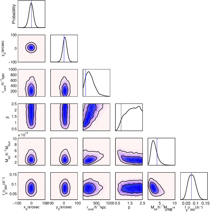
Figs. 13 and 14 represent the marginalised posterior distributions from the analysis of simulated SZ cluster data for sampling and derived parameters respectively while in Table 10 we present the mean, the dispersion and the maximum likelihood of each cluster parameter estimated using parameterisation III.
| Parameter | ||
|---|---|---|
The strong degeneracy between and is quite apparent in this parameterisation, while is poorly constrained and biased towards higher values. We note that, since the SZ analysis constrains cluster total mass internal to the radius and we use the virial M-T relation (equation (33)) to derive cluster average temperature within this radius, the result of temperature estimation is less biased and more reliable than the parameterisations I and II in recovering the temperature true value. We have used this parameterisation in our follow-up analysis of the real data where we studied a joint weak gravitational lensing and SZ analysis of six clusters (AMI Consortium: Hurley- Walker et al. 2011) and high and moderate X-ray luminosity sample of LoCuSS clusters (AMI Consortium: Rodríguez-Gonzálvez et al. 2011; AMI Consortium: Shimwell et al. 2011).
8.4 Analysis using entropy-GNFW pressure model
Similar to the isothermal -model we first studied our methodology for the ”entropy”-GNFW pressure model with no data. The results are represented in Figs. 15 and 16. This analysis again helps us understand which parameters are constrained by SZ measurement as well as to check the algorithm in retrieving the prior probability distributions. From both 1-D and 2-D marginalised probability distributions it is clear that we are able to recover the input priors probability distributions and the probability distributions of the derived parameters are according to their corresponding functional dependencies on the sampling parameters.
Figs. 17, 18 and Table 11 show the results of our analysis for ”entropy” -GNFW pressure profile using parameterisation II while Figs. 19, 20 and Table 12 show the results of the same analysis using parameterisation III. We note that in both analyses and the parameters that define the shape of the entropy profile are not constrained while the scaling radius, , which defines the GNFW pressure profile is completely constrained. As a result we notice similar constraints in the estimation of in both parameterisations since we assume a fixed . We also note the degeneracies between - and - which are because of the dependency of on these two free parameters. On the other hand the - degeneracy seen in Figs. 17 and 19 is due to the intrinsic degeneracy that exists between the cluster size and the volume integrated Comptonisation parameter (- degeneracy) in the SZ measurements (Planck Collaboration 2011d). Moreover, comparing and (Table 11 and 12) confirms a radial decline in the ICM temperature distribution as expected.
Overall, both parameterisations could constrain the cluster physical parameters, however, analysis using parameterisation III leads to a tighter constrain on both and . The results of Parameterisation III once more show that this parameterisation can reliably be used in the analysis of clusters of galaxies as it is less model dependent and produces unbiased results in particular when the assumption of hydrostatic equilibrium breaks, in young or disturbed clusters (parameterisation II).


| Parameter | ||
|---|---|---|


| Parameter | ||
|---|---|---|
9 Discussion and Conclusions
We have studied two parameterised models, the traditional isothermal -model and the “entropy”-GNFW pressure model, to analyse the SZ effect from galaxy clusters and extract their physical parameters using AMI SA simulated data. In our analysis we have described the current assumptions made on the dynamical state of the ICM including spherical geometry, hydrostatic equilibrium and the virial mass-temperature relation. In particular we have shown how different parameterisations which relate the thermodynamical quantities describing the ICM to the cluster global properties via these assumptions lead to biases on the cluster physical parameters within a particular model.
In this context, we first generated a simulated cluster using the isothermal -model observed with the AMI SA and used these simulated data to study three different parameterisations in deriving the cluster physical parameters. We showed that in generating AMI simulated data, it is extremely important to select the model parameters describing the SZ signal in a way that leads to the consistent cluster parameter inferences upon using the three different parameterisation methods.
We found that each parameterisation introduces different constraints and biases in the posterior probability distribution of the inferred cluster parameters which arise from the way we implement assumptions about the cluster structure and its composition. The biases in the posterior probability distributions of the cluster parameters are more pronounced in parameterisations I and II, as the results depend strongly on the relatively unconstrained cluster model shape parameters: and . However, the biases introduced by the choice of priors are even worse in parameterisation I, in which the gas temperature is assumed to be an independent free parameter. This, along with the assumption of isothermality, causes the priors to dominate in extracting the cluster physical parameters regardless the type of prior chosen for the gas temperature (AMI Consortium: Rodríguez-Gonzálvez et al. 2011 and AMI Consortium: Zwart et al. 2010). The cluster physical parameters estimated using parameterisation I depend strongly on the model parameters. Although it can constrain the cluster position and its , it fails to recover the true input values of most of the simulated cluster properties. For example the inferred values for mass and temperature at are and whereas the corresponding input values of simulated cluster are: and . In terms of the application to the real data, we have noticed similar biases in the results of our analysis of 7 clusters using this parameterisation (AMI Consortium: Zwart et al. 2010). In order to improve our analysis methodology in parameterisations II and III, the correlation between the cluster total mass and its gas temperature is taken into account. In parameterisation II we relate and using the hydrostatic equilibrium whereas in parameterisation III we use virial mass-temperature relationship. It should be noted that the derived in parameterisation II is the gas temperature at the overdensity radius which is then assumed to be constant throughout the cluster. In parameterisation III, however, is the mean gas temperature internal to radius and is assumed to be constant. We notice that analysing the same simulated data set using parameterisation II can constrain the 1-D posterior distribution of the cluster physical parameters better than parameterisation I such that and . Since parameterisation II uses the full parametric hydrostatic equilibrium, the temperature estimate depends on and and is therefore biased low. These results were also confirmed in our analysis of the bullet like cluster A2146 (AMI Consortium: Rodríguez-Gonz álvezet al. 2011). Relating the cluster total mass and its temperature via virial theorem in parameterisation III leads to less bias in cluster physical parameters compared to the other two parameterisations as it is less model dependent: and .
A detailed comparison between our different parameterisations both using simulated data and on the bullet like cluster A2146 (AMI Consortium: Rodríguez-Gonzálvez et al. 2011) found that parameterisation III can give more reliable results for cluster physical properties as it is less dependent on model parameters. Parameterisation II also gives convincing estimates for the cluster total mass and its gas content although its temperature estimate is poorly justified, as it depends strongly on the model parameters. Moreover, young or disturbed clusters are unlikely to be well-described by hydrostatic equilibrium. We therefore used parameterisation III as our adopted analysis methodology in our follow-up studies of the real clusters including the joint SZ and weak lensing analysis of six clusters (AMI Consortium: Hurley-Walker et al. 2011) and the analysis of LoCuss cluster sample (AMI Consortium: Rodríguez-Gonz álvez et al. 2011; AMI Consortium: Shimwell et al. 2011).
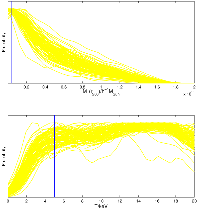
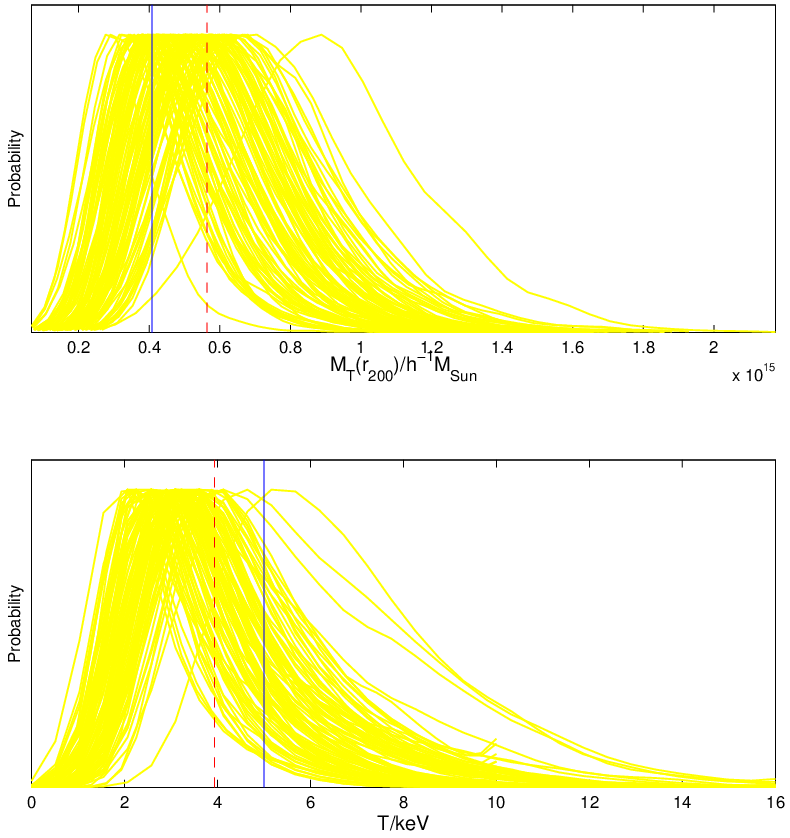
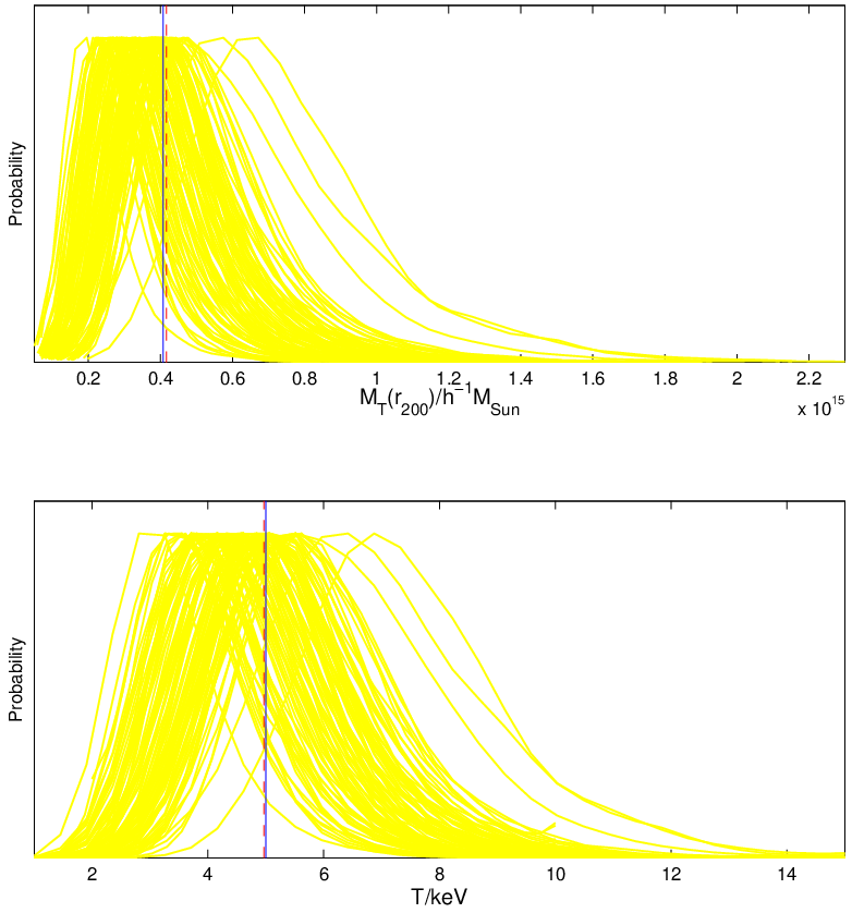
In order to make sure that our results are not biased by one realisation of primordial CMB, we have studied CMB realisations for the three parameterisations. The 1-D marginalised posterior probability distributions of and are shown in Figs. 21, 22 and 23 for each parameterisation. The solid blue line represents the true value corresponding to the simulated cluster and the dashed red line shows the mean value of the distributions. Table 13 also presents the numerical results of this analysis.
| parameterisation | ||
|---|---|---|
| I | ||
| II | ||
| III |
Comparing the 1D posterior distributions along with the mean values of the estimates in the three parameterisations for these realisations show that parameterisation I can hardly constrain the simulated cluster properties and recover the input true values. Parameterisation II can constrain the cluster total mass, however, the gas temperature estimate is biased low as it depends on unconstrained model shape parameters. On the other hand, parameterisation III can indeed constrain both cluster mass and its gas temperature and the results are unbiased.
In order to remove the assumption of isothermality which is of course a poor assumption both within the cluster inner region and at the large radii and to improve our analysis model for the cluster ICM which can be fitted accurately throughout the cluster, we also studied the SZ effect using “entropy”-GNFW pressure model. This model assumes a 3-D -model like radial profile describing the entropy in the ICM as well as the GNFW profile for the plasma pressure. This choice is reasonable as the entropy is a conserved quantity and describes the structure of the ICM while the pressure is related to the dark matter component of the cluster. Moreover, among all the thermodynamical quantities describing the ICM, entropy and pressure show more self- similar distribution in the outskirts of the cluster. The combination of these two profiles then allows us to relate the SZ observable properties to the cluster physical parameters such as its total mass. This model also allows the electron pressure and its number density profiles to have different distributions leading to a 3-D radial temperature profile. In this context we simulated a second cluster using an entropy-GNFW pressure profile with the same physical parameters and thermal noise as the first cluster at .
We then analysed the second simulated cluster using ”entropy”-GNFW pressure model with different parameterisations. In this model temperature is no longer isothermal so that we can not use parameterisation I where a single temperature is assumed as an independent input parameter. The results of our analysis using parameterisation II and III show that while the characteristic scaling radius describing the GNFW pressure profile is constrained, the shape parameters defining the entropy profile remain unconstrained. Moreover, all the cluster physical parameters lie within errorbars from the corresponding true values of the simulated cluster in the two parameterisations. However, parameterisation III provides tighter constrains in 1-D marginalised posterior distribution of the temperature and the overall results are less model dependent so that it can be reliably used in the analysis of galaxy clusters in particular when the assumption of hydrostatic equilibrium breaks (e.g. in disturbed clusters and clusters that are going through merging).
We conclude that using the “entropy”-GNFW pressure model overcomes the limitations of the isothermal -model in fitting cluster parameters over a broad radial extent. However, AMI simulated data do not strongly prefer one model over the other. We investigated this conclusion further by fitting both GNFW pressure profile and isothermal -model to a simulated cluster with and . The result is shown in Fig. 24 with blue dashed line representing the fit using the isothermal -model and the red representing the fit using GNFW pressure profile. However, we aim to compare these two models in our future studies using the real data.

Acknowledgments
The analysis work was conducted on the Darwin Supercomputer of the University of Cambridge High Performance Computing Service supported by HEFCE. The authors thank Stuart Rankin for computing assistance. We also thank Dave Green for his invaluable help with LaTeX. MO, CRG, MLD, TMOF, MPS and TWS acknowledge PPARC/STFC studentships.
References
- Afshordi & Cen (2002) Afshordi N., Cen R., 2002, ApJ, 564, 669
- Afshordi et al. (2007) Afshordi N., Lin Y.-T., Nagai D., Sanderson A. J. R., 2007, MNRAS, 378, 293
- Allison et al. (2011) Allison J. R., Taylor A. C., Jones M. E., Rawlings S., Kay S. T., 2011, MNRAS, 410, 341
- AMI Consortium: Hurley-Walker et al. (2011) AMI Consortium: Hurley-Walker N. et al., 2011, arXiv,:1101.5912
- AMI Consortium: Rodríguez-Gonzálvez et al. (2011) AMI Consortium: Rodríguez-Gonzálvez C. et al., 2011, MNRAS, 661
- AMI Consortium: Rodríguez-Gonzálvez et al. (2011) AMI Consortium: Rodríguez-Gonzálvez C. et al., 2011, arXiv:1101.5589
- AMI Consortium: Shimwell et al. (2010) AMI Consortium: Shimwell T. et al., 2010, arXiv:1012.4441
- AMI Consortium: Shimwell et al. (2011) AMI Consortium: Shimwell T. et al., 2011, arXiv:1101.5590
- AMI Consortium: Zwart et al. (2008) AMI Consortium: Zwart J. T. L., et al., 2008, MNRAS, 391, 1545
- AMI Consortium: Zwart et al. (2011) AMI Consortium: Zwart J. T. L., et al., 2011, MNRAS, 1931
- Andersson et al. (2011) Andersson K., et al., 2011, ApJ, 738, 48
- Arnaud, Pointecouteau, & Pratt (2005) Arnaud M., Pointecouteau E., Pratt G. W., 2005, A&A, 441, 893
- Arnaud et al. (2010) Arnaud M., Pratt G. W., Piffaretti R., Böhringer H., Croston J. H., Pointecouteau E., 2010, A&A, 517, A92
- Bartlett & Silk (1994) Bartlett J. G., Silk J., 1994, ApJ, 423, 12
- Bautz et al. (2009) Bautz M. W., et al., 2009, PASJ, 61, 1117
- Birkinshaw (1999) Birkinshaw M., 1999, PhR, 310, 97
- Böhringer et al. (2007) Böhringer H. et al., 2007, A&A, 469, 363
- Borgani et al. (2004) Borgani S., et al., 2004, MNRAS, 348, 1078
- Borgani (2004) Borgani S., 2004, Ap&SS, 294, 51
- Carlstrom, Holder, & Reese (2002) Carlstrom J. E., Holder G. P., Reese E. D., 2002, ARA&A, 40, 643
- Cavaliere & Fusco-Femiano (1976) Cavaliere A., Fusco-Femiano R., 1976, A&A, 49, 137
- Cavaliere & Fusco-Femiano (1978) Cavaliere A., Fusco-Femiano R., 1978, A&A, 70, 677
- Challinor & Lasenby (1998) Challinor A., Lasenby A., 1998, ApJ, 499, 1
- da Silva et al. (2004) da Silva A. C., Kay S. T., Liddle A. R., Thomas P. A., 2004, MNRAS, 348, 1401
- Eke et al. (1998) Eke V. R., Cole S., Frenk C. S., Patrick Henry J., 1998, MNRAS, 298, 1145
- Eke, Navarro, & Frenk (1998) Eke V. R., Navarro J. F., Frenk C. S., 1998, ApJ, 503, 569
- Ettori et al. (2009) Ettori S., Morandi A., Tozzi P., Balestra I., Borgani S., Rosati P., Lovisari L., Terenziani F., 2009, A&A, 501, 61
- Evrard, Metzler, & Navarro (1996) Evrard A. E., Metzler C. A., Navarro J. F., 1996, ApJ, 469, 494
- Evrard et al. (2002) Evrard A. E., et al., 2002, ApJ, 573, 7
- Feroz & Hobson (2008) Feroz F., Hobson M. P., 2008, MNRAS, 384, 449
- Feroz, Hobson, & Bridges (2009) Feroz F., Hobson M. P., Bridges M., 2009, MNRAS, 398, 1601
- Feroz et al. (2009) Feroz F., Hobson M. P., Zwart J. T. L., Saunders R. D. E., Grainge K. J. B., 2009, MNRAS, 398, 2049
- Finoguenov, Reiprich, Böhringer (2001) Finoguenov A., Reiprich T. H., Böhringer H., 2001, A&A, 368, 749
- Finoguenov (2002) Finoguenov A., 2002, ASPC, 253, 71
- Fixsen et al. (1996) Fixsen D. J., Cheng E. S., Gales J. M., Mather J. C., Shafer R. A., Wright E. L., 1996, ApJ, 473, 576
- George et al. (2009) George M. R., Fabian A. C., Sanders J. S., Young A. J., Russell H. R., 2009, MNRAS, 395, 657
- Grainge et al. (2002) Grainge K., Jones M. E., Pooley G., Saunders R., Edge A., Grainger W. F., Kneissl R., 2002, MNRAS, 333, 318
- Grego et al. (2001) Grego L., Carlstrom J. E., Reese E. D., Holder G. P., Holzapfel W. L., Joy M. K., Mohr J. J., Patel S., 2001, ApJ, 552, 2
- Hallman et al. (2007) Hallman E. J., Burns J. O., Motl P. M., Norman M. L., 2007, ApJ, 665, 911
- Hobson & Maisinger (2002) Hobson M. P., Maisinger K., 2002, MNRAS, 334, 569
- Hoshino et al. (2010) Hoshino A., et al., 2010, PASJ, 62, 371
- Kawaharada et al. (2010) Kawaharada M., et al., 2010, ApJ, 714, 423
- Itoh, Kohyama, & Nozawa (1998) Itoh N., Kohyama Y., Nozawa S., 1998, ApJ, 502, 7
- Jones et al. (1993) Jones M., et al., 1993, Natur, 365, 320
- Kaiser (1986) Kaiser N., 1986, MNRAS, 222, 323
- Komatsu et al. (2011) Komatsu E., et al., 2011, ApJS, 192, 18
- Kravtsov & Gnedin (2005) Kravtsov A. V., Gnedin O. Y., 2005, ApJ, 623, 650
- Kravtsov, Nagai, & Vikhlinin (2005) Kravtsov A. V., Nagai D., Vikhlinin A. A., 2005, ApJ, 625, 588
- Kravtsov, Vikhlinin, & Nagai (2006) Kravtsov A. V., Vikhlinin A., Nagai D., 2006, ApJ, 650, 128
- Larson et al. (2011) Larson D., et al., 2011, ApJS, 192, 16
- Lewis, Challinor, & Lasenby (2000) Lewis A., Challinor A., Lasenby A., 2000, ApJ, 538, 473
- Lloyd-Davies, Ponman, & Cannon (2000) Lloyd-Davies E. J., Ponman T. J., Cannon D. B., 2000, MNRAS, 315, 689
- Mason & Myers (2000) Mason B. S., Myers S. T., 2000, ApJ, 540, 614
- Maughan (2007) Maughan B. J., 2007, ApJ, 668, 772
- Maughan et al. (2007) Maughan B. J., Jones C., Jones L. R., Van Speybroeck L., 2007, ApJ, 659, 1125
- McCarthy, Bower, & Balogh (2007) McCarthy I. G., Bower R. G., Balogh M. L., 2007, MNRAS, 377, 1457
- Mitchell et al. (2009) Mitchell N. L., McCarthy I. G., Bower R. G., Theuns T., Crain R. A., 2009, MNRAS, 395, 180
- Mroczkowski et al. (2009) Mroczkowski T., et al., 2009, ApJ, 694, 1034
- Nagai (2006) Nagai D., 2006, ApJ, 650, 538
- Nagai, Kravtsov, & Vikhlinin (2007) Nagai D., Kravtsov A. V., Vikhlinin A., 2007, ApJ, 668, 1
- Nagai & Lau (2011) Nagai D., Lau E. T., 2011, ApJ, 731, L10
- Nagai (2011) Nagai D., 2011, MmSAI, 82, 594
- Nozawa, Itoh, & Kohyama (1998) Nozawa S., Itoh N., Kohyama Y., 1998, ApJ, 508, 17
- Piffaretti & Valdarnini (2008) Piffaretti R., Valdarnini R., 2008, A&A, 491, 71
- Plagge et al. (2010) Plagge T., et al., 2010, ApJ, 716, 1118
- Planck Collaboration et al. (2011) Planck Collaboration, et al., 2011, A&A, 536, A12
- Placnk Collaboration et al. (2011) Placnk Collaboration, et al., 2011, A&A, 536, A11
- Planck Collaboration et al. (2011) Planck Collaboration, et al., 2011, A&A, 536, A10
- Planck Collaboration et al. (2011) Planck Collaboration, et al., 2011, A&A, 536, A9
- Planck Collaboration et al. (2011) Planck Collaboration, et al., 2011, A&A, 536, A8
- Pointecouteau, Giard, & Barret (1998) Pointecouteau E., Giard M., Barret D., 1998, A&A, 336, 44
- Pointecouteau, Arnaud, & Pratt (2005) Pointecouteau E., Arnaud M., Pratt G. W., 2005, A&A, 435, 1
- Ponman, Cannon, & Navarro (1999) Ponman T. J., Cannon D. B., Navarro J. F., 1999, Nature, 397, 135
- Ponman, Sanderson, & Finoguenov (2003) Ponman T. J., Sanderson A. J. R., Finoguenov A., 2003, MNRAS, 343, 331
- Pratt & Arnaud (2002) Pratt G. W., Arnaud M., 2002, A&A, 394, 375
- Pratt, Arnaud, & Pointecouteau (2006) Pratt G. W., Arnaud M., Pointecouteau E., 2006, A&A, 446, 429
- Pratt, Arnaud, & Pointecouteau (2006) Pratt G. W., Arnaud M., Pointecouteau E., 2006, ESASP, 604, 695
- Pratt et al. (2010) Pratt G. W., et al., 2010, A&A, 511, A85
- Press & Schechter (1974) Press W. H., Schechter P., 1974, ApJ, 187, 425
- Reiprich et al. (2009) Reiprich T. H., et al., 2009, A&A, 501, 899
- Rephaeli (1995) Rephaeli Y., 1995, ARA&A, 33, 541
- Sanderson & Ponman (2003) Sanderson A. J. R., Ponman T. J., 2003, MNRAS, 345, 1241
- Sanderson et al. (2003) Sanderson A. J. R., Ponman T. J., Finoguenov A., Lloyd-Davies E. J., Markevitch M., 2003, MNRAS, 340, 989
- Sarazin (1988) Sarazin C. L., 1988, X–ray Emission from Clusters of Galaxies, Cambridge University Press
- Sarazin (2008) Sarazin C. L., 2008, LNP, 740, 1
- Simionescu et al. (2011) Simionescu A., et al., 2011, Sci, 331, 1576
- Skilling (2004) Skilling J., 2004,AIP Conf.Proc.,735, 395
- Sunyaev & Zeldovich (1970) Sunyaev R. A., Zeldovich Y. B., 1970, CoASP, 2, 66
- Tozzi & Norman (2001) Tozzi P., Norman C., 2001, ApJ, 546, 63
- Urban et al. (2011) Urban O., Werner N., Simionescu A., Allen S. W., Böhringer H., 2011, MNRAS, 414, 2101
- Vikhlinin et al. (2005) Vikhlinin A., Markevitch M., Murray S. S., Jones C., Forman W., Van Speybroeck L., 2005, ApJ, 628, 655
- Vikhlinin et al. (2006) Vikhlinin A., Kravtsov A., Forman W., Jones C., Markevitch M., Murray S. S., Van Speybroeck L., 2006, ApJ, 640, 691
- Voit (2000) Voit G. M., 2000, ApJ, 543, 113
- Voit & Ponman (2003) Voit G. M., Ponman T. J., 2003, ApJ, 594, L75
- Voit (2004) Voit G. M., 2004, IAU Colloq. 195: Outskirts of Galaxy Clusters: Intense Life in the Suburbs, ogci.conf, 253
- Voit (2005) Voit G. M., 2005, RvMP, 77, 207
- Wadsley, Veeravalli, & Couchman (2008) Wadsley J. W., Veeravalli G., Couchman H. M. P., 2008, MNRAS, 387, 427
- Yoshikawa, Jing, & Suto (2000) Yoshikawa K., Jing Y. P., Suto Y., 2000, ApJ, 535, 593