Calibration Using Matrix Completion with Application to Ultrasound TomographyThanks:  Reza Parhizkar, Amin Karbasi and Martin Vetterli are with the School of Computer and Communication Sciences, Ecole Polytechnique Fédérale de Lausanne (EPFL), CH-1015 Lausanne, Switzerland (e-mails: {reza.parhizkar, amin.karbasi, martin.vetterli}@epfl.ch). Sewoong Oh is with the Laboratory for Information and Decision Systems, MIT, MA 02139, USA (e-mail: swoh@mit.edu). Martin Vetterli is also with the Department of Electrical Engineering and Computer Sciences, University of California, Berkeley, CA 94720, USA.Thanks: This work has been partly presented in the conference proceeding [1].Thanks: This work was supported by the Swiss National Science Foundation under grants 200021-121935 and ERC Advanced Grant–Support for Frontier Research–SPARSAM, Nr: 247006.

In most applications involving sensing, finding the correct positions of the sensors is of crucial importance for obtaining reliable results. This is particularly true in the case of inverse problems which can be very sensitive to incorrect sensor placement. This requirement can be satisfied in two ways; One might put the effort in the construction of the instruments and try to place the sensors exactly in the desired positions, or use a method to find the exact positions after the construction of the device. In this work we will consider the latter and we call the procedure of obtaining the sensor positions calibration. Note that even in the former case, due to the precision of the construction instruments, a calibration is needed afterwards for determining the exact sensor positions. Although in rare cases a single calibration might be enough throughout the lifetime of the measurement system, it is of great use to have a calibration procedure which can be repeated easily and with low cost.

This work focusses on the calibration problem in circular sensing devices, in particular, the ones manufactured and deployed in  [2, 3]. These devices consist of a circular ring surrounding an object and scanning horizontal planes. Ultrasound sensors are placed on the interior boundary of the ring and act both as transmitters and receivers.

The calibration problem we address in this paper is the following; In the circular tomography devices, the sensors are not exactly placed on a perfect circle. This uncertainty in the positions of the sensors acts as a source of error in the reconstruction algorithms used to obtain the characteristics of the enclosed object. We aim at finding a simple method for calibrating the system with correct sensor positions with low cost and without using any extra calibrating instrument.

In order to find the correct sensor positions, we incorporate the time-of-flight (ToF) of ultrasound signals between pairs of sensors, which is the time taken by an ultrasound wavefront to travel from a transmitter to a receiver. If we have all the ToF measurements between all pairs of sensors when the enclosed medium is homogeneous, then we can construct a ToF matrix where each entry corresponds to the ToF between each pair of sensors. We can infer the positions of the sensors using this ToF matrix.

To obtain reliable ToF entries appropriate for our purpose, we assume that no object is placed inside the ring during the calibration phase and prior to actual measurements. There are a number of challenges we are encountering in this work, namely,

• •

  the ToF matrices obtained in a practical setup have missing entries.

• •

  the measured entries of the ToF matrices are corrupted by noise.

• •

  there is an unknown time delay added to the measurements.

If one had the complete and noiseless ToF matrix without time delay, the task of finding the exact positions would be very simple. This problem is addressed in literature as multi-dimensional scaling (MDS) [4]. Unfortunately, the ToF matrix in practical setups is never complete and many of the time-of-flight values are missing. The missing entries can be divided into two categories; structured missing entries caused by inability of the sensors to compute the mutual time-of-flights with their close-by neighbors, and random missing entries due to malfunctioning of the sensors or the ToF estimation algorithm during the measurement procedure.

A good estimation of the positions of the sensors can be obtained, if we have a good estimation of the missing entries of the ToF matrix. In general, it is a difficult task to infer missing entries of a matrix. However, it has recently been established that if the matrix is low rank, a small random subset of its entries permits an exact reconstruction [5]. Since a modified version of the ToF matrix (when the entries are squared ToF measurements) is low rank, its missing entries can be accurately estimated using matrix completion algorithms. To this end, we use OptSpace , a robust matrix completion algorithm developed by Keshavan et al. [6].

On top of the missing entries, we also need to deal with an unknown time delay. This delay it due to the fact that in practice, the impulse response of the piezoelectric and the time origin in the measurement procedure are not known, and this causes an unknown time delay which should then be added to the measurements. To infer this time delay simultaneously with the positions of the sensors, we propose a heuristic algorithm based on OptSpace.

In circular setups, the sensors are not necessarily on a circle and deviate from the circumference which in fact motivates the calibration problem. We therefore need to assume that they are in the proximity of a circle (the precise statement is given later) and we are required to find the exact positions. Our approach is to estimate the local and random missing pairwise distances from which we can then infer the positions. As we have already mentioned, we show that a modified version of the ToF matrix has rank at most four, and using this property, we propose our calibration procedure. The block diagram shown in Fig. 1 summarizes the procedure.

The focus of this research is ultrasound tomography with circular apertures. In this setup, $n$ ultrasound transmitters and receivers are installed on the interior edge of a circular ring and an object with unknown acoustic characteristics is placed inside the ring. At each time instance a transmitter is fired, sending ultrasound signals with frequencies ranging from hundreds to thousands of kHz, while the rest of the sensors record the received signals. The same process is repeated for all the transmitters. Each one of $n$ sensors on the ring is capable of transmitting and receiving ultrasound signals. The aim of tomography in general is to use the recorded signals in order to reconstruct the characteristics of the enclosed object (e.g. sound speed, sound attenuation, etc.). The general configuration for such a tomography device is depicted in Fig. 3. Employing these measurements, an inverse problem is constructed, whose solution provides the acoustic characteristics of the enclosed object.

There are two common methods for solving the inverse problem. The solutions are either based on the wave equation [21] or the bent-ray theory [22]. Both techniques consist of forward modeling the problem and comparing the simulation results with the measured data. For the details see [21] and [22]. Nevertheless, in both cases, in order to simulate the forward model and rely on the recorded data, a very precise estimate of the sensor positions is needed. In most applications (e.g., [23, 24, 25]) it is assumed that the sensors are positioned equidistant apart on a circle and no later calibration is performed to find the exact sensor positions. The main objective of this paper is to estimate the precise positions of the sensors.

We observed that the distance matrix, when the aperture is in homogeneous medium, is calculated as in (1). We also saw in the previous section that the measurements for the ToF matrix $\bm{T}$ have three major problems : they are noisy, some of them are missing, and the measurements contain some unknown time delay. For simplicity, we will assume that this time delay is constant for all the transmitters, namely all the transmitters send the electrical signal after some fixed but unknown delay $t_{0}$. Hence, we can rewrite the ToF matrix as follows

where $\bm{T}$ consists of ideal measurements for ToF, $\bm{Z}_{0}$ is the noise matrix and $\bm{A}$ is defined as

With the above considerations, the distance matrix can also be written as

where $\bm{D}=c_{0}\bm{T}$, $d_{0}=c_{0}t_{0}$, and $\bm{Z}=c_{0}\bm{Z}_{0}$.

In our model we do not assume that the sensors are placed exactly on the ring. What happens in practice is that the sensor positions deviate from the circumference and our ultimate goal is to estimate these deviations or equivalently the correct positions (see Fig. 6). The general positions taken by sensors are denoted by the set of vectors $\{\bm{x}_{1},\ldots,\bm{x}_{n}\}$.

As described earlier, there are two contributions to missing entries. One is the missing measurements of close-by sensors, which we call structured missing entries. The other is the missing measurements due to random malfunction of sensors, which we call random missing entries. First, to incorporate the structured missing entries, we assume that any measurements between sensors of distance less than $\delta_{n}$ are missing (see Figure 6). Hence, the number of structured missing entries depends on $\delta_{n}^{2}$. We are interested in the regime where we have a small number of structured missing entries per row in the large systems limit. Accordingly, typical range of $\delta_{n}$ of interest is $\delta_{n}=\Theta(\,r\sqrt{\log n/n})$. A random set of structured missing indices $S\subseteq[n]\times[n]$ is defined from $\{\bm{x}_{i}\}$ and $\delta_{n}$, by

where $d_{i,j}=\left\|\bm{x}_{i}-\bm{x}_{j}\right\|$. Then, the structured missing entries are denoted by a matrix

Note that the matrix $\bm{D}^{\bar{s}}=\bm{D}-\bm{D}^{s}$ captures the noiseless distance measurements that is not effected by structured missing entries. This way, we can interpret the matrix $\bm{D}^{s}$ as additive noise in our model. Likewise, for the constant additive time delay we can define

where $S^{\perp}$ denotes the complementary set of $S$. Next, to model the noise we add a random noise matrix $\bm{Z}^{\bar{s}}$.

We do not assume a prior distribution on $\bm{Z}$, and the main theorem is stated for any general noise matrix $\bm{Z}$, deterministic or random. One practical example of $\bm{Z}$ is an i.i.d. Gaussian model.

Finally, to model the random missing entries, we assume that each entry of $\bm{D}^{\bar{s}}+t_{0}c_{0}\bm{A}^{\bar{s}}+\bm{Z}^{\bar{s}}$ is sampled with probability $p_{n}$. In the calibration data, we typically see a small number of random missing entries. Hence, in order to model it we assume that $p_{n}=\Theta(1)$. Let $E\subseteq[n]\times[n]$ denote the subset of indices which are not erased by random missing entries. Then a projection ${\cal P}_{E}:\mathbb{R}^{n\times n}\to\mathbb{R}^{n\times n}$ is defined as

We denote the observed measurement matrix by

where $d_{0}=t_{0}c_{0}$ is a constant. Notice that the matrix $\bm{N}^{E}$ has the same shape as $\bm{T}_{{}_{\text{inc}}}$ shown already schematically in Fig. 5. Now we can state the goal of our calibration problem:

Given the observed matrix $\bm{N}^{E}$ and the missing indices $S\cup E^{\perp}$, we want to estimate a matrix $\widehat{\bm{D}}$ which is close to the correct distance matrix $\bm{D}$. Then by using $\widehat{\bm{D}}$ we would like to estimate the sensor positions.

In order to achieve this goal, there are two obstacles we need to overcome. First, we need to estimate the missing entries of $\bm{N}^{E}$ and second, we want to find the sensor positions given approximate pairwise distances. The former is done by employing a matrix completion algorithm and the latter by using the multidimensional scaling method.

OptSpace, introduced in [17], is an algorithm for recovering a low-rank matrix from noisy data with missing entries. The steps are shown in Algorithm 1. Let $\bm{M}$ be a rank-$q$ matrix of dimensions $n\times n$, $\bm{Z}$ the measurement noise, and $E$ the set of indices of the measured entries. Then, the measured noisy and incomplete matrix is $\bm{M}^{E}={\cal P}_{E}(\bm{M}+\bm{Z})$.

In the trimming step, a row or a column is over-represented if it contains more samples than twice the average number of samples per row or column. These rows or columns can dominate the spectral characteristics of the observed matrix $\bm{M}^{E}$. Thus, some of their entries are removed uniformly at random from the observed matrix. Let $\widetilde{\bm{M}}^{E}$ be the resulting matrix of this trimming step. This trimming step is presented here for completeness, but in the case when $p_{n}$ is larger than some fixed constant (like in our case where $p_{n}=\Theta(p)$), $\bm{M}^{E}$=$\widetilde{\bm{M}}^{E}$ with high probability and the trimming step can be omitted.

In the second step, we first compute the singular value decomposition (SVD) of $\widetilde{\bm{M}}^{E}$.

where $\sigma_{i}(\cdot)$ denotes the $i$-th singular value of a matrix. Then, the rank-$q$ projection returns the matrix

obtained by setting to $0$ all but the $q$ largest singular values.

Starting from the initial guess provided by the rank-$q$ projection ${\cal P}_{q}(\widetilde{\bm{M}}^{E})$, the final step solves a minimization problem stated as the following [17]:
Given $\bm{X}\in\mathbb{R}^{n\times q},\bm{Y}\in\mathbb{R}^{n\times q}$ with $\bm{X}^{T}\bm{X}=\bm{1}$ and $\bm{Y}^{T}\bm{Y}=\bm{1}$, define

Values for $\bm{X}$ and $\bm{Y}$ are computed by minimizing $F(\bm{X},\bm{Y})$. This consists of writing ${\cal P}_{q}(\widetilde{\bm{M}}^{E})=\bm{X}_{0}\bm{S}_{0}Y_{0}^{T}$ and minimizing $F(\bm{X},\bm{Y})$ locally with initial condition $\bm{X}=\bm{X}_{0}$ and $\bm{Y}=\bm{Y}_{0}$. This last step tries to get us as close as possible to the correct low rank matrix $\bm{M}$.

Even if we had a good estimate of $\bm{D}$, how we would position the sensors is not a trivial question. Multidimensional scaling (MDS) is a technique used in finding the configuration of objects in a low dimensional space such that the measured pairwise distances are preserved. If all the pairwise distances are measured without error, then a naive application of MDS exactly recovers the configuration of sensors [28, 12, 4].

There are various types of MDS techniques, but, throughout this paper, by MDS we refer to the classical metric MDS, which is defined as follows. Let $\bm{L}$ be an $n\times n$ symmetric matrix such that

where ${\mathds{1}}_{n}\in\mathbb{R}^{n}$ is the all ones vector and ${\mathbb{I}}_{n}$ is the $n\times n$ identity matrix. Let ${\sf MDS}_{\eta}(\bar{\bm{D}})$ denote the $n\times{\eta}$ matrix returned by MDS when applied to the squared distance matrix $\bar{\bm{D}}$. The task is to embed $n$ objects in a ${\eta}$ dimensional space $\mathbb{R}^{\eta}$. In our case for instance, where we want to find the position of sensors on a two dimensional space, we have ${\eta}=2$. Then, in the equation, given the singular value decomposition (SVD) of a symmetric and positive semidefinite matrix $(-1/2)\bm{L}\bar{\bm{D}}\bm{L}$ as $(-1/2)\bm{L}\bar{\bm{D}}\bm{L}=\bm{U}\bm{\Sigma}\bm{U}^{T}$,

where $\bm{U}_{\eta}$ denotes the $n\times{\eta}$ left singular matrix corresponding to the ${\eta}$ largest singular values and $\bm{\Sigma}_{\eta}$ denotes the ${\eta}\times{\eta}$ diagonal matrix with ${\eta}$ largest singular values in the diagonal. This is also known as the MDSLocalize algorithm in [4]. Note that since the columns of $\bm{U}$ are orthogonal to ${\mathds{1}}_{n}$ by construction, it follow that

It can be easily shown that when MDS is applied to the correct and complete squared distance matrix without noise, the configuration of sensors are exactly recovered [4]. This follows from

where $\bm{X}$ denotes the $n\times{\eta}$ position matrix in which the $i$-th row corresponds to $\bm{x}_{i}$, the ${\eta}$ dimensional position vector of sensor $i$. Note that we only get the configuration and not the absolute positions, in the sense that ${\sf MDS}_{\eta}(\bar{\bm{D}})$ is one version of infinitely many solutions that matches the distance measurements $\bm{D}$. Intuitively, it is clear that the pairwise distances are invariant to a rigid transformation (a combination of rotation, reflection and translation) of the positions $\bm{X}$, and therefore there are multiple instances of $\bm{X}$ that result in the same $\bm{D}$. For future use, we introduce a formal definition of rigid transformation and related terms.

Denote by ${\sf O}({\eta})$ the group of orthogonal ${\eta}\times{\eta}$ matrices. A set of sensor positions $\bm{Y}\in\mathbb{R}^{n\times{\eta}}$ is a rigid transform of $\bm{X}$, if there exists a ${\eta}$-dimensional shift vector $\bm{s}$ and an orthogonal matrix $\bm{Q}\in{\sf O}({\eta})$ such that

$\bm{Y}$ should be interpreted as a result of first rotating (and/or reflecting) sensors in position $\bm{X}$ by $\bm{Q}$ and then adding a shift by $\bm{s}$. Similarly, when we say two position matrices $\bm{X}$ and $\bm{Y}$ are equal up to a rigid transformation, we mean that there exists a rotation $\bm{Q}$ and a shift $\bm{s}$ such that $\bm{Y}=\bm{X}\bm{Q}+{\mathds{1}}_{n}\bm{s}^{T}$. Also, we say a function $f(\bm{X})$ is invariant under rigid transformation if and only if for all $\bm{X}$ and $\bm{Y}$ that are equal up to a rigid transformation, we have $f(\bm{X})=f(\bm{Y})$. Under these definitions, it is clear that $\bm{D}$ is invariant under rigid transformation, since for all $(i,j)$, $\bm{D}_{ij}=\left\|\bm{x}_{i}-\bm{x}_{j}\right\|=\left\|(\bm{x}_{i}\bm{Q}+\bm{s}^{T})-(\bm{x}_{j}\bm{Q}+\bm{s}^{T})\right\|\;$, for any $\bm{Q}\in{\sf O}({\eta})$ and $\bm{s}\in\mathbb{R}^{\eta}$.

Let $\widehat{\bm{X}}$ denote an $n\times{\eta}$ estimation for $\bm{X}$ with estimated position for sensor $i$ in the $i$-th row. Then, we need to define a metric for the distance between the original position matrix $\bm{X}$ and the estimation $\widehat{\bm{X}}$ which is invariant under rigid transformation of $\bm{X}$ or $\widehat{\bm{X}}$.

The matrix $\bm{L}$ defined in (5) is a symmetric matrix with rank $n-1$ which eliminates the contributions of the translation. More precisely,

for all $\bm{s}\in R^{\eta}$. We can show that $\bm{L}$ has the following properties.

This naturally defines the following distance between $\bm{X}$ and $\widehat{\bm{X}}$.

where $\left\|\cdot\right\|_{F}$ denotes the Frobenius norm.

According to Lemma 2, this distance is invariant to rigid transformation of $\bm{X}$ and $\widehat{\bm{X}}$. Furthermore, $d(\bm{X},\widehat{\bm{X}})=0$ implies that $\bm{X}$ and $\widehat{\bm{X}}$ are equal up to a rigid transformation. We later state our theoretical results in terms of the distance defined in (8).

We saw that the OptSpace algorithm is not directly applicable to the squared distance matrix because of the unknown delay. Since $\bm{A}$ in (2) is a full rank matrix, the matrix $\widetilde{\bm{D}}\odot\widetilde{\bm{D}}=[{\tilde{d}_{i,j}}^{2}]$ no longer has rank four. Moreover, since the measurements are noisy, one cannot hope for estimating the exact value for $d_{0}$. Therefore, in the following we will provide error bounds on the reconstruction of the positions assuming that the time delay (equivalently $d_{0}$) is known. Afterwards, a heuristic method is proposed to estimate the value of $d_{0}$.

In Table I the set of important notations used in the sequel is summarized.

The above theorem, in great generality, holds for any noise matrix $\bm{Z}$, deterministic or random. The above guarantees only hold ‘up to numerical constants’. To see how good OptSpace is in practice, we need to run numerical experiments. For more results supporting the robustness of OptSpace, we refer to [18].

In Algorithm 3, we propose a heuristic method for estimating the value of $d_{0}$ along with completion of the squared distance matrix.

In fact, this algorithm guarantees that after removing the effect of the time delay, we have found the best rank 4 approximation of the distance squared matrix. In other words, if we remove exactly the mismatch $d_{0}$, we will have an incomplete version of a rank 4 matrix and after reconstruction, the measured values will be close to the reconstructed ones.

This section is dedicated to the proof of our main result. To do so we apply Theorem 1.2 of [6] to the rank-$4$ matrix $\bar{\bm{D}}$ and the observed matrix $\bm{N}^{E}={\cal P}_{E}(\bar{\bm{D}}-\bar{\bm{D}}^{s}+\bm{Z}^{\bar{s}})$.

First, we provide the definition of a crucial property of $\bar{\bm{D}}$ which is called incoherence. Following the definition in [6], a rank-$4$ symmetric matrix $\bar{\bm{D}}\in\mathbb{R}^{n\times n}$ is said to be $\mu$-incoherent if the following conditions hold. Let $U\Sigma U^{T}$ be the singular value decomposition of $\bar{\bm{D}}$.

• A0.

  For all $i\in[n]$, we have $\sum_{k=1}^{4}{U_{i,k}^{2}}\leq 4\mu/n$.

• A1.

  For all $i\in[n]$, $j\in[n]$, we have $\big|\bar{\bm{D}}_{i,j}/\sigma_{1}(\bar{\bm{D}})\big|\leq\sqrt{4}\mu/n$.

The extra $1/n$ terms in the right hand side are due to the fact that, in this paper, we assume that the singular vectors are normalized to unit norm, whereas in [6] the singular vectors are normalized to have norm $\sqrt{n}$.

Theorem 1.2 of [6] states that if a rank-$4$ matrix $\bar{\bm{D}}$ is $\mu$-incoherent then the following is true with probability at least $1-1/n^{3}$. Let $\sigma_{i}(\bar{\bm{D}})$ be the $i$th singular value of $\bar{\bm{D}}$ and $\kappa(\bar{\bm{D}})=\sigma_{1}(\bar{\bm{D}})/\sigma_{4}(\bar{\bm{D}})$ be the condition number of $\bar{\bm{D}}$. Also, let $\widehat{\bar{\bm{D}}}$ denote the estimation returned by OptSpace with input $N^{E}={\cal P}_{E}(\bar{\bm{D}}-\bar{\bm{D}}^{s}+\bm{Y}^{\bar{s}})$. Then, there exists numerical constants $C_{1}$ and $C_{2}$ such that

provided that

and

First, using Lemma 3, we show that the bound in (11) gives the desired bound in the theorem. Then, it is enough to show that there exists a numerical constant $N$ such that the conditions in (12) and (13) are satisfied with high probability for $n\geq N$.

Now, to show that (12) holds with high probability for $n\geq C\log n/p$ for some constant $C$, we show that $\kappa\leq f_{\kappa}(r_{0},a)$ and $\mu\leq f_{\mu}(r_{0},a)$ with high probability, where $f_{\kappa}$ and $f_{\mu}$ are independent of $n$. Recall that $\kappa(\bar{\bm{D}})=\sigma_{1}(\bar{\bm{D}})/\sigma_{4}(\bar{\bm{D}})$. We have

where $\rho_{i}$ is distributed in such a way that we have uniform distribution over the circular band. Thus, one can show that

where

One can write $\bm{S}$ as

It follows that $\sigma_{1}(\bar{\bm{D}})\leq\frac{r_{0}+\sqrt{1+r_{0}^{2}}}{r_{0}}\sigma_{1}(\bm{A}\bm{A}^{T})$ and $\sigma_{4}(\bar{\bm{D}})\geq\min\Big(2,\frac{\sqrt{1+r_{0}^{2}}-r_{0}}{r_{0}}\Big)\sigma_{4}(\bm{A}\bm{A}^{T})$. We can compute the expectation of this matrix over the distribution of node positions. Having uniform distribution of the sensors over the circular ring, we have for the probability distribution of $\rho$:

Thus, the expectation of the matrix $\bm{A}^{T}\bm{A}$ is easily computed as

Let the largest and smallest singular values of $\mathbb{E}[\bm{A}^{T}\bm{A}]$ to be $n\sigma_{\max}(r_{0},a)$ and $n\sigma_{\min}(r_{0},a)$. Using the fact that $\sigma_{i}(\cdot)$ is a Lipschitz continuous function of its arguments, together with the Chernoff bound for large deviation of sums of i.i.d. random variables, we get

for some constant $C$. Hence, with high probability, $\kappa(\bar{\bm{D}})\leq\frac{4\sigma_{\max}(r_{0},a)}{\sigma_{\min}(r_{0},a)}=f_{\kappa}(r_{0},a)$.

Now to bound $\mu$, note that with probability $1$ the columns of $\bm{A}$ are linearly independent. Therefore, there exists a matrix $\bm{B}\in\mathbb{R}^{r\times r}$ such that $\bm{A}=\bm{V}\bm{B}^{T}$ with $\bm{V}^{T}\bm{V}={\mathds{I}}$. The SVD of $\bar{\bm{D}}$ then reads $\bar{\bm{D}}=\bm{U}\Sigma\bm{U}^{T}$ with $\Sigma=\bm{Q}^{T}\bm{B}^{T}\bm{S}\bm{B}\bm{Q}$ and $\bm{U}=\bm{V}\bm{Q}$ for some orthogonal matrix $\bm{Q}$. To show incoherence property A0, we need to show that, for all $i\in[n]$,

Since $\bm{V}_{i}=\bm{B}^{-1}\bm{A}_{i}$, we have $\|\bm{V}_{i}\|^{2}\leq\sigma_{4}(\bm{B})^{-2}\|\bm{A}_{i}\|^{2}\leq\sigma_{4}(\bm{A})^{-2}\|\bm{A}_{i}\|^{2}$. Combined with $\|\bm{A}_{i}\|^{2}=r_{0}^{2}+(r_{0}+\rho_{i})^{2}+(2r_{0}\rho_{i}+\rho_{i}^{2})^{2}\leq r_{0}^{2}+(r_{0}+a)^{2}+(2r_{0}a+a^{2})^{2}$ and (16), we have

with high probability, where $f_{\mu}(r_{0},a)=2(r_{0}^{2}+(r_{0}+a)^{2}+(2r_{0}a+a^{2})^{2})$.

To show incoherence property A1, we use $|\bar{\bm{D}}_{ij}|\leq(2r_{0}+a)^{2}$ and $\sigma_{1}(\bar{\bm{D}})\geq\frac{1}{4}n\,\sigma_{\min}(r_{0},a)\min\left(2,\frac{\sqrt{1+r_{0}^{2}}-r_{0}}{r_{0}}\right)$ from (15). Then,

with high probability, where $g(r_{0},a)=\max\left(2,\frac{4r_{0}}{\sqrt{1+r_{0}^{2}}-r_{0}}\right)(2r_{0}+a)^{2}/\sigma_{\min}(r_{0},a)$. Combining (17) and (18), we see that the incoherence property is satisfied, with high probability.

Further, (13) holds, with high probability, if the right-hand side of (9) is less than $C_{3}\frac{\sqrt{1+r_{0}^{2}}+r_{0}}{r_{0}}\sigma_{\max}(r_{0},a)$, since $\sigma_{4}(\bar{\bm{D}})\leq\frac{1}{2}n\frac{\sqrt{1+r_{0}^{2}}+r_{0}}{r_{0}}\sigma_{\max}(r_{0},a)$. This finishes the proof of Theorem 1.

$\blacksquare$

In order to evaluate the performance of the calibration method, three sets of experiments are done. First, the distance matrix is assumed noiseless and the value of the $d_{0}$ is set to zero. The position estimation error is derived for different values of $n$ and the ring width $a$. The value of $r_{0}$ is set to $10$ cm, on average 5 percent of entries are missing randomly, and $\delta$ in Theorem 1 is assumed to be 1. For each value of $a$ and $n$, the experiment is repeated 10 times, and the average is taken. The results are reported in Fig. 7. As expected from Corollary 1, the greneral trend in all curves is that the error decreases as $n$ grows. Moreover, the larger $a$ is, the bigger is the reconstruction error, which is also coherent with the results of Corollary 1.

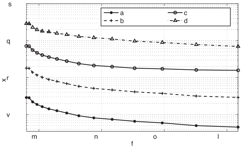
To examine the stability of the estimation algorithm under noise, we set the values of $a$ to $1$ cm, $\delta$ to $1$, $r_{0}$ to $10$ cm, $t_{0}$ to zero, and the percentage of random missing entries to 5. We added to each entry of the distance matrix $\bm{D}$ a centred white Gaussian noise of different standard deviations. For each $n$ and standard deviation of noise, the experiments are repeated 10 times and the average is taken. The results are depicted in Fig. 8 ¹¹ 1 There has been a slight mislabeling in the earlier version of this paper in [1] which is corrected in this paper. . As the variance of the noise increases, the position estimation error grows, but in general the error decreases for larger $n$.

As we discussed in Section I-A, one might treat the calibration problem as a special case of the sensor localization problem. However, there is a duality between the calibration problem and the traditional sensor localization problems. We showed in Section II that in the calibration problem the local distance/connectivity information is not available whereas most of the state-of-the-art algorithms for sensor localization are based on the local information. In order to compare the performance of these methods with the proposed methods, a set of simulations are performed. We compared the localization results of our method to the ones of Mds-Map [12], Sdp-based [14] and also Svd-Reconstruct [4]. The position reconstruction error (defined in (8)) versus the number of sensors, $n$ for the methods is reported in Fig. 9 in a log-log scale.

For the simulations, we set the values of $a$ to 1 cm, $\delta$ to 1, $r_{0}$ to 10 cm, $t_{0}$ to zero, and the percentage of the random missing entries to 5. The distance measurements were corrupted with a white Gaussian noise of standard deviation $0.6$ mm. For each method and each $n$, the experiment is performed 10 times for different positions and different noises, and the average error is taken. For the Sdp-based method, we have used the algorithm presented in [14] and the code published by the same authors. For Mds-Map, we have estimated the shortest paths using Johnson’s algorithm [29]. Finally for Svd-Reconstruct, we used the algorithm in [4]. In order to adapt the measurements with the assumptions of the method, we assumed that $p_{ij}=1-0.05=0.95$ for the measured points (note that $0.05$ is on average the probability of having a random missing entry) and $\gamma_{ij}=0$.

As the results in Fig. 9 suggest, Mds-Map and Svd-Reconstruct methods perform very bad compared to the other two methods. The poor performance of Mds-Map is for the fact that it highly relies on the presence of local distance information, whereas in our case, these measurements are in fact missing. This method is based on estimating the missing distance measurements with the shortest path between the two sensors. However, one can easily see that given faraway sensor distances, the shortest path is a very coarse approximation of the distance between close-by sensors. also note that as the simulation results show, there is no guarantee that the estimation error will decrease as $n$ grows.

For Svd-Reconstruct, the unrealistic assumption that all the sensors have a non-zero probability of being connected causes the bad results of the method. In our case, the probability that the close-by sensors are connected is zero because of the structured missing entries. In fact, since $p_{ij}$ is high, one could see this method as simply applying the classical MDS on the incomplete distance matrix. The surprising observation about the performance of this method is that the estimation error does not change much with $n$.

In contrast to the two aforementioned algorithms, the Sdp-based method performs very well for estimating the sensor positions and the reconstruction error is very close to the one of the proposed method. The reason is the fact that this method does not directly rely on the local distance information. In fact, the distance measurements are fed to the algorithm as the constraints of a convex optimization problem. However, as the number of sensors goes large, the number of measurements also grows and so does the number of constraints for the semi-definite program. This causes the method not to work for $n$ larger than 150 in our case. The same limitation is also reported by the authors of the method.

In summary, taking the computational cost and reconstruction accuracy of the algorithms into account, the proposed method performs significantly better.

Moreover, to show the importance of calibration in an ultrasound scanning device, a simple simulation is also performed. If the ToF measurements correspond to the exact positions of sensors without time delay $t_{0}$, reconstruction of water will lead to a homogeneous region with values equal to the water sound speed, whereas wrong assumption on the sensor positions and $t_{0}$ causes the inverse method to give incorrect values as the sound speed to compensate the effect of position mismatch.

In a simple experiment, we simulated the reconstruction of water sound speed ($c_{0}=1500$) using the ToF measurements. In the simulation, 200 sensors are distributed around a circle with radius $r_{0}=10$ cm, and they deviate at most $5$ mm from the circumference and the ToF measurements are added by $t_{0}=10\mu s$. The incomplete distance matrix is shown in Fig. 10(a).

In order to complete the distance matrix and find the time delay at the same time, we used Algorithm 3. We forced the rank of $\bar{\bm{D}}$ to 4. The value for $t_{0}$ is found as $4\mu s$ which is exactly as set in the simulation. The output of OptSpace algorithm is the completed $\bar{\bm{D}}$ matrix which is shown in Fig. 10(b).

Using the completed distance matrix and the MDS method, the positions are reconstructed and fed to an inverse tomography algorithm to reconstruct water sound speed. The results of the reconstruction are shown in Fig. 11. In the figure, the results for four reconstructions are presented. In Fig. 11, the ToF matrix is not complete, it contains the time delay $t_{0}$, and the positions are not calibrated. The dark gray ring is caused by the non-zero time delay in the ToF measurements. In Fig. 11, the time mismatch is resolved using the proposed algorithm, but the sensor positions are not calibrated and the ToF matrix is still not complete. This figure shows clearly that finding the unknown time delay improves significantly the reconstruction image. Figure 11, shows the reconstructed medium when the ToF matrix is completed and time mismatch is removed, but the sensor positions are not yet calibrated. From this figure, it is confirmed that accurate time-of-flights are necessary but not sufficient to have a good reconstruction of the inclosed object. Finally, Fig. 11 shows the reconstruction when the positions are also calibrated. Notice the change in the dynamic range for the last case.

In this work we introduced a theoretical framework for calibration in circular ultrasound tomography devices. We proposed a novel calibration algorithm for which we provided theoretical bounds on the performance. We also tested our method through exhaustive simulations to demonstrate its functionality in practice. We compared the algorithm with some state-of-the-art centralized sensor localization methods and showed that our method outperforms those in estimating the correct sensor positions.

Even though we introduced a recursive algorithm for finding the time-delay, we were not able to provide theoretical guarantees on its convergence. We mainly observed its convergence through simulations. This is still an interesting theoretical challenge and requires further work. We also believe that our approach can potentially be deployed beyond circular to other popular topologies with simple geometry.

References

- [1] R. Parhizkar, A. Karbasi, and M. Vetterli, “Calibration in circular ultrasound tomography devices,” in Acoustics, Speech and Signal Processing (ICASSP), 2011 IEEE International Conference on, may 2011, pp. 549 –552.
- [2] N. Duric, P. Littrup, L. Poulo, A. Babkin, R. Pevzner, E. Holsapple, O. Rama, and C. Glide, “Detection of breast cancer with ultrasound tomography: First results with the computed ultrasound risk evaluation (cure) prototype,” Medical Physics, vol. 34, no. 2, pp. 773–785, 2007.
- [3] I. Jovanovic, L. Sbaiz, and M. Vetterli, “Acoustic tomography for scalar and vector fields: theory and application to temperature and wind estimation,” Journal of Atmospheric and Oceanic Technology, vol. 26, no. 8, pp. 1475 – 1492, 2009.
- [4] P. Drineas, A. Javed, M. Magdon-Ismail, G. Pandurangant, R. Virrankoski, and A. Savvides, “Distance matrix reconstruction from incomplete distance information for sensor network localization,” in Sensor and Ad Hoc Communications and Networks, vol. 2, Sept. 2006, pp. 536–544.
- [5] E. J. Candès and B. Recht, “Exact matrix completion via convex optimization,” CoRR, vol. abs/0805.4471, 2008.
- [6] R. H. Keshavan, A. Montanari, and S. Oh, “Matrix completion from noisy entries,” in Advances in Neural Information Processing Systems, December 2009.
- [7] T. He, C. Huang, B. M. Blum, J. A. Stankovic, and T. Abdelzaher, “Range-free localization schemes for large scale sensor networks,” in MobiCom ’03, 2003, pp. 81–95.
- [8] S. Čapkun, M. Hamdi, and J. Hubaux, “GPS-free positioning in mobile ad hoc networks,” Cluster Computing, vol. 5, no. 2, pp. 157–167, 2002.
- [9] C. Liu, K. Wu, and T. He, “Sensor localization with ring overlapping based on comparison of received signal strength indicator,” IEEE Inter. Conf. on Mobile Ad-hoc and Sensor Systems, pp. 516–518, 2004.
- [10] D. Niculescu and B. Nath, “Ad hoc positioning system (APS) using AoA,” in INFOCOM, vol. 3, 2003, pp. 1734–1743.
- [11] A. Savvides, C. Han, and M. Strivastava, “Dynamic fine-grained localization in ad-hoc networks of sensors,” in Proceedings of the 7th MobiCom, 2001, pp. 166–179.
- [12] Y. Shang, W. Ruml, Y. Zhang, and M. P. J. Fromherz, “Localization from mere connectivity,” in MobiHoc ’03. ACM, 2003, pp. 201–212.
- [13] S. Oh, A. Montanari, and A. Karbasi, “Sensor network localization from local connectivity: Performance analysis for the mds-map algorithm,” in ITW 2010, 2010, pp. 1–5.
- [14] P. Biswas, T. chen Liang, K. chuan Toh, T. chung Wang, and Y. Ye, “Semidefinite programming approaches for sensor network localization with noisy distance measurements,” IEEE Transactions on Automation Science and Engineering, vol. 3, p. 2006, 2006.
- [15] A. Javanmard and A. Montanari, “Localization from incomplete noisy distance measurements,” Mar 2011, arXiv:1103.1417v3.
- [16] P. Drineas, A. Javed, M. Magdon-Ismail, G. Pandurangant, R. Virrankoski, and A. Savvides, “Distance matrix reconstruction from incomplete distance information for sensor network localization,” in SECON ’06, vol. 2, 2006, pp. 536–544.
- [17] R. H. Keshavan, A. Montanari, and S. Oh, “Matrix completion from a few entries,” IEEE Trans. Inform. Theory, 2010, arXiv:0901.3150.
- [18] R. H. Keshavan and S. Oh, “OptSpace: A gradient descent algorithm on the grassman manifold for matrix completion,” IEEE Trans. Inform. Theory, 2009, arXiv:0910.5260.
- [19] B. Recht, “A simpler approach to matrix completion,” Arxiv preprint arXiv:0910.0651, 2009.
- [20] B. Recht, W. Xu, and B. Hassibi, “Null space conditions and thresholds for rank minimization,” Math. Program., vol. 127, no. 1, pp. 175–202, Mar 2011.
- [21] F. Natterer and F. Wübbeling, Mathematical Methods in Image Reconstruction. SIAM, 2001.
- [22] I. Jovanović, “Inverse problems in acoustic tomography,” Ph.D. dissertation, EPFL, Lausanne, 2008.
- [23] I. Jovanović, A. Hormati, L. Sbaiz, and M. Vetterli, “Efficient and stable acoustic tomography using sparse reconstruction methods,” in 19th International Congress on Acoustics, 2007.
- [24] F. Simonetti, L. Huang, and N. Duric, “On the spatial sampling of wave fields with circular ring apertures,” Journal of Applied Physics, vol. 101, no. 8, p. 083103, 2007.
- [25] F. Natterer, “Acoustic mammography in the time domain,” University of Münster, Germany, Tech. Rep., 2008.
- [26] C. Li, L. Huang, N. Duric, H. Zhang, and C. Rowe, “An improved automatic time-of-flight picker for medical ultrasound tomography,” Ultrasonics, vol. 49, no. 1, pp. 61 – 72, 2009.
- [27] J. Chen, Y. Huang, and J. Benesty, “Time delay estimation,” in Audio Signal Processing for Next-Generation Multimedia Communication Systems, Y. Huang and J. Benesty, Eds. Springer US, 2004, ch. 8, pp. 197–227.
- [28] J. B. Kruskal and M. Wish, Multidimensional scaling. SAGE Publications, 1978.
- [29] D. B. Johnson, “Efficient algorithms for shortest paths in sparse networks,” J. ACM, vol. 24, pp. 1–13, January 1977.
-A Proof of Lemma 1
The proof for the general case where the sensors are not on a circle is provided in [4]. In the circular case however, we have , where is the circle radius. Thus, the squared distance matrix is decomposable to
where
This finishes the proof.
-B Proof of Corollary 1
Note that in general has rank at most where is the dimension of the space in which sensors are placed (in our case ). Therefore,
where we used the fact that for any matrix of rank we have . Furthermore, the spectral norm can be bounded in terms of and as follows.