Experience Rating with Poisson Mixtures

Throughout our discussion, $n$ will denote the number of data points and $k$ will denote the number of components in the mixture formulation. For a finite mixture model, the observed likelihood function is

where the weights are non-negative and $\sum_{j=1}^{k}w_{j}=1$. Even for moderate values of $n$ and $k$, this takes a long time to evaluate since there are $k^{n}$ terms when the inner sums are expanded (Casella et al., 2000). Another form of the likelihood function will be derived shortly. Classical estimation procedures for mixture models are described by Titterington et al. (1990) and McLachlan and Peel (2000).

Let $z_{i}$ be a categorical random variable taking values in $\{1,\ldots,k\}$ with probabilities $w_{1},\ldots,w_{k}$, respectively, so that

Suppose that the conditional distribution of $D_{i}$, given $z_{i}=j$, is $Poisson(\lambda_{j})$, $j=1,\ldots,k$. Let $f_{j}(\cdot)$ denote a Poisson density with parameter $\lambda_{j}$. Then the unconditional density of $D_{i}$ is given by $f(D_{i})$, where

With every pair $(D_{i},E_{i})$, we associate a latent variable $z_{i}$, which is an indicator variable that indicates which component of the mixture is associated with $(D_{i},E_{i})$. We have, $z_{i}=j$ if the $i^{th}$ data point, $(D_{i},E_{i})$, comes from the $j^{th}$ component of the mixture. Thus, for each $i$, we have

and

By incorporating the indicator variables $z$, the complete data likelihood is then

At times, especially for the fixed $k$ case described below, it is more convenient to work with (3) as it involves multiplications only, rather than additions and multiplications, as in (1).

The convenience of using the missing data formulation is that the posterior conditional distribution of the model parameters would be standard distributions. Also the augmented variables $z$ allows us to see what component of the mixture the data points are assigned.

We consider a mixture of Poissons where, conditional on there being $k$ components in the mixture, we have

The weights $w_{j}$ sum to one, and are non–negative, so that

and

follows a Dirichlet distribution. We also make the additional assumption that the $\delta_{j}$’s are equal to $1$ so that $p(w)$ is a uniform distribution on the space described by (4). For the Poisson parameters $\lambda_{j}$, we take Gamma priors, so that

with the ordering constraint

to ensure that the components are identifiable. The ordering constraint is not necessary for the Monte Carlo algorithm to work. However it does avoid the problem of label switching, since otherwise, any permutation of the indices $\{1,\ldots,k\}$ will result in the same posterior distribution.

Note that because we have the ordering constraint in Equation (5), the joint density of the collective $\lambda$ is

When $k$ is fixed and known, the factorial term $k!$ does not affect the MCMC algorithm since it can be absorbed into the normalising constant. However, in the variable $k$ case, it must be noted, since it is a factor in the reversible jump acceptance probability. The joint density of all unknowns is

With the missing data formulation, the likelihood term $\hbox{\boldmath$L$}(D^{n}|\lambda,z,E^{n})$ can be written

and

where $n_{j}=\#\{i|z_{i}=j\}$, is the number of observations allocated to component $j$. The prior distributions are

Using Bayes’ theorem, we have the following posterior conditional distributions:

and

so that,

where $n_{j}=\#\{i|z_{i}=j\}$. For $z$, we update the allocations using

so that,

This follows from Equation (2). The Gibbs algorithm for fixed $k$ is then (Robert and Casella, 1999)

Step 1:

Simulate $z_{i}$ from

$$p(z_{i}=j)\propto w_{j}f(D_{i}|\lambda_{j},E_{i})\text{ for $j=1,\ldots,k$}$$

and compute $n_{j}$, $n_{j}\bar{D}_{j}$, $n_{j}\bar{E}_{j}$ from

$$n_{j}=\sum_{i|z_{i}=j}(1)\quad n_{j}\bar{D}_{j}=\sum_{i|z_{i}=j}D_{i}\quad n_{j}\bar{E}_{j}=\sum_{i|z_{i}=j}E_{i}$$

Step 2:

Simulate

$$\lambda_{j}\sim\mathcal{G}amma(\alpha+n_{j}\bar{D}_{j},\beta+n_{j}\bar{E}_{j})\mathbb{I}_{(\lambda_{j-1},\lambda_{j+1})}(\lambda_{j})\text{ for $j=1,\ldots,k$}$$

Step 3:

Simulate

$$w\sim\mathcal{D}(\delta+n_{1},\ldots,\delta+n_{k}).$$

The Reversible jump algorithm is an extension of the Metropolis–Hastings algorithm. We assume there is a countable collection of candidate models, indexed by $M\in\mathcal{M}=\{M_{1}$, $M_{2}$,$\ldots$ , $M_{k}\}$. We further assume that for each model $M_{i}$, there exists an unknown parameter vector $\hbox{\boldmath$\theta$}_{i}\in\mathbb{R}^{n_{i}}$ where $n_{i}$, the dimension of the parameter vector, can vary with $i$. Typically we are interested in finding which models have the greatest posterior probabilities and also estimates of the parameters. Thus the unknowns in this modelling scenario will include the model index $M_{i}$ as well as the parameter vector $\hbox{\boldmath$\theta$}_{i}$. We assume that the models and corresponding parameter vectors have a joint density $\pi(M_{i},\hbox{\boldmath$\theta$}_{i})$. The reversible jump algorithm constructs a reversible Markov chain on the state space $\mathcal{M}\times\bigcup_{M_{i}\in\mathcal{M}}\mathbb{R}^{n_{i}}$ which has $\pi$ as its stationary distribution (Green, 1995). In many instances, and in particular for Bayesian problems this joint distribution is of the form

where the prior on $(M_{i},\hbox{\boldmath$\theta$}_{i})$ is often of the form

with $p(M_{i})$ being the density of some counting distribution.

Suppose now that we are at model $M_{i}$ and a move to model $M_{j}$ is proposed with probability $r_{ij}$. The corresponding move from $\hbox{\boldmath$\theta$}_{i}$ to $\hbox{\boldmath$\theta$}_{j}$ is achieved by using a deterministic transformation $h_{ij}$, such that

where $u$ and $v$ are random variables introduced to ensure dimension matching necessary for reversibility. To ensure dimension matching we must have

For discussions about possible choices for the function $h_{ij}$ we refer the reader to Green (1995), and Brooks et al. (2003). Let

then the acceptance probability for a proposed move from model $(M_{i},\hbox{\boldmath$\theta$}_{i})$ to model $(M_{j},\hbox{\boldmath$\theta$}_{j})$ is

where $q(\hbox{\boldmath$u$})$ and $q(\hbox{\boldmath$v$})$ are the respective proposal densities for $u$ and $v$, and $\lvert\partial h_{ij}(\hbox{\boldmath$\theta$}_{i},\hbox{\boldmath$u$})/\partial(\hbox{\boldmath$\theta$}_{i},\hbox{\boldmath$u$})\rvert$ is the Jacobian of the transformation induced by $h_{ij}$. Green (1995) shows that the algorithm with acceptance probability given above simulates a Markov chain which is reversible and follows from the detailed balance equation

Detailed balance is necessary to ensure reversibility and is a sufficient condition for the existence of a unique stationary distribution. For the reverse move from model $M_{j}$ to model $M_{i}$ it is easy to see that the transformation used is $(\hbox{\boldmath$\theta$}_{i},\hbox{\boldmath$u$})=h_{ij}^{-1}(\hbox{\boldmath$\theta$}_{j},\hbox{\boldmath$v$})$ and the acceptance probability for such a move is

For inference regarding which model has the greater posterior probability we can base our analysis on a realisation of the Markov chain constructed above. The marginal posterior probability of model $M_{i}$

where

is the marginal density of the data after integrating over the unknown parameters $\theta$. In practice we estimate $\pi(M_{i}|\hbox{\boldmath$X$})$ by counting the number of times the Markov chain visits model $M_{i}$ in a single long run after reaching stationarity. These between model moves described in this section are also augmented with within model Gibbs updates as given in Section 4.2 to update model parameters.

Note that the joint density in Equation (10) now depends on $k$. We use the split/merge method of Dellaportas et al. (1997) and Viallefont et al. (2002). Suppose we are at a configuration with $k$ components, let

and suppose a move to increase the number of components is proposed. We select uniformly one of the current $k$ components to be split. Suppose the $j^{th}$ component, $(\lambda_{j},w_{j})$, is selected to be split into two components $(\lambda_{j_{1}},w_{j_{1}})$ and $(\lambda_{j_{2}},w_{j_{2}})$ such that $j_{1}=j$ and $j_{2}=j+1$, the components originally numbered $j+1,\ldots,k$ are then renumbered $j+2,\ldots,k+1$. The split is also designed so that the first two moments of the split component remains the same as the original component. Thus, we simulate $u_{1}$ and $u_{2}$ from densities defined on the interval $[0,1]$. Usually, we use Beta densities and set

Other choices for splitting and merging components are described in Viallefont et al. (2002). The proposed parameter is then

If the ordering constraint in Equation (5) is not satisfied then the move is rejected immediately, as the reverse move in which we merge two adjacent components would not be possible. We can compute the Jacobian for this transformation as

For the reverse move, we select a pair of adjacent components $j_{1}$ and $j_{2}$. Combining them, to get a new component labelled $j$, we set

by keeping the first two moments of the proposed and current configuration constant. We then sample a new set of allocation variables according to Equation (7). We also keep track of the probability of each allocation, so that $p_{a}(z)$ represents the probability of a given allocation. To compute $p_{a}(z)$, we first simulate $z_{i}$ using Equation (7). For each $i$, the probability of that allocation is given by

Finally, we compute the probability of all allocations by

The acceptance probability of a move of type $(k,\hbox{\boldmath$\theta$}_{k})\Rightarrow(k^{\prime},\hbox{\boldmath$\theta$}_{k^{\prime}})$ is then $\min\{1,A_{k,k^{\prime}}\}$, where

With $k^{\prime}=k+1$ this becomes

Now with a uniform prior on the number of components $k$ and the weights $w$,

where the ratio of Gamma terms comes from the ratio of the prior distributions on $w^{\prime}$ and $w$ and

Suppose we are now at model $M_{k}$ with $k$ components, say

If a move is proposed to increase the number of components by one, then we simulate

independently. The proposed new component will then have weight $\tilde{w}$ and the other weights are then scaled by a factor of $(1-\tilde{w})$, so that the sum of the weights remain $1$. The corresponding Poisson parameter for the proposed component in $\tilde{\lambda}$. Note that $\tilde{\lambda}$ is sampled from its prior distribution. The proposed component is then

Using this proposed value of $\hbox{\boldmath$\theta$}_{k+1}$, we also simulate proposed values for the allocations $z^{\prime}$ with model $k+1$. Using the general form of the reversible jump acceptance probability, see for example Green (1995)), the probability of changing the number of components to $k+1$ is then $\min\{1,A_{k,k+1}\}$, where

Making the necessary substitutions yield

Using Equations (12) and (13) we then have the Jacobian

If we denote the probability of a birth when there are $k$ components by $b_{k}$, and the probability of a death by $d_{k}$, with $b_{k}+d_{k}=1$, then

since for the move to be reversible we would then be able to kill $k+1$ components in the new model, each with equal probability. Substituting these values in Equation (14), the ratio $A_{k,k+1}$ reduces to

which on substituting $q(\tilde{\lambda})=p(\tilde{\lambda})$ and $q(\tilde{w})=k(1-\tilde{w})^{k-1}$ further reduces to

For a proposed death move, the acceptance probability is then

Even though the algorithm simulates new values of for the allocations when proposing to move, it is not necessary to carry the allocations along. For between–model moves, we could replace the missing data formulation by noting that

Thus we could update model parameters using a scheme which does not require conjugacy; see for example Cappé et al. (2003a); Cappé et al. (2003b).

A comparison of the individual acceptance probabilities shows that the between model moves are accepted with a larger rate for the birth death scheme compared with the split merge scheme. This might not always be true, as other split merge schemes may be proposed (Viallefont et al., 2002). It is interesting to note that although the birth and death rates are higher than the split and merge rates, the combined scheme seems to mix better than either scheme implemented alone. Even though the birth and death scheme have a higher acceptance rate for between–model moves, the excursions away from the values of highest posterior density, $k=2$ and $k=3$, are longer than for the combined scheme or the split and merge scheme since. This is because when proposing parameters independently from the prior, areas of low probability can be proposed, whereas, with the split and merge scheme, areas of low probability mass will generally be rejected. Based on the results presented here, the birth/death method would be the preferred algorithm.

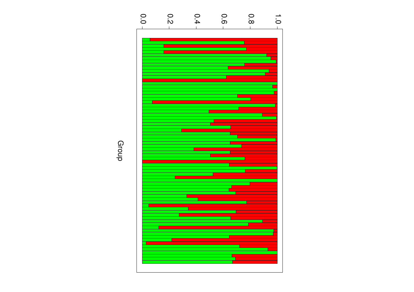
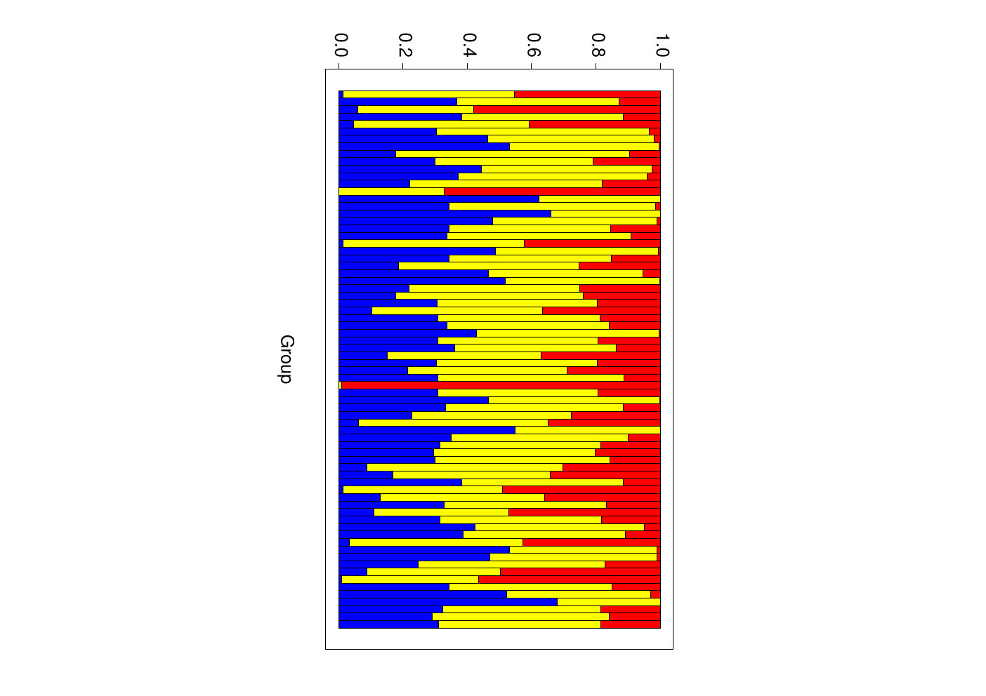
A histogram plot of the model indicator from the reversible jump algorithm of Section 5 shows that the most plausible model generating the claims in the portfolio is a mixture of two Poisson distributions. In this section we look further at the results, conditional on their being only two components, or three components, in the mixture.

Recall the missing data formulation introduced in Section 4 for the number of components conditional on $k=2$, we observed the posterior distribution of $z$ at each iteration when $k=2$. A study of values of $z$ will tell us how the data has been allocated to the components and therefore, which data points have been generated from either the first Poisson distribution or the second Poisson distribution. This information, along with further information from the portfolio, will help insurance companies classify groups of life insurance portfolios. The parameter estimates are shown in Table 3.

Similar results for the posterior parameter estimates, conditional on there being three components in the mixture, are given in Table 4.

Figure 5 show the posterior probability of each data point being allocated to a particular component of the mixture, conditional on $k=2$ and conditional $k=3$, respectively.

References

- Brooks et al. (2003) Brooks, S. P., P. Giudici, and G. O. Roberts (2003). Efficient construction of reversible jump MCMC proposal distributions (with discussion). Journal of the Royal Statistical Society, Series B 65(1), 3–55.
- Cappé et al. (2003a) Cappé, O., C. P. Robert, and T. Rydén (2003a). CT/RJ-Mix: Transdimensional MCMC for Gaussian mixtures (available as C source code).
- Cappé et al. (2003b) Cappé, O., C. P. Robert, and T. Rydén (2003b). Reversible jump, birth–and–death and more general continuous time Markov chain Monte Carlo samplers. Journal of the Royal Statistical Society, Series B 65(3), 679–700.
- Carlin and Chib (1995) Carlin, B. P. and S. Chib (1995). Bayesian Model Choice via Markov chain Monte Carlo methods. Journal of the Royal Statistical Society, Series B 57, 473–484.
- Casella et al. (2000) Casella, G., C. P. Robert, and M. T. Wells (2000). Mixture Models, Latent Variables and Partitioned Importance Sampling. Technical Report 2000–03, CREST, INSEE, Paris.
- Dellaportas and Karlis (2001) Dellaportas, P. and D. Karlis (2001). A simulation approach to nonparametric empirical Bayes analysis. International Statistical Review 69(1), 63–79.
- Dellaportas et al. (1997) Dellaportas, P., D. Karlis, and E. Xekalaki (1997). Bayesian analysis of finite Poisson mixtures. Technical report, Athens University of Economics and Business.
- Green (1995) Green, P. J. (1995). Reversible jump Markov chain Monte Carlo computation and Bayesian model determination. Biometrika 82(4), 711–732.
- Green and Richardson (2001) Green, P. J. and S. Richardson (2001). Modelling heterogeneity with and without the Dirichlet process. Scandinavian Journal of Statistics 28(2), 355–375.
- Green and Richardson (2002) Green, P. J. and S. Richardson (2002). Hidden Markov Models and Disease Mapping. Journal of the American Statistical Society 97(460), 1055–1070.
- Haastrup (2000) Haastrup, S. (2000). Comparison of Some Bayesian Analyses of Heterogeneity in Group Life Insurance. Scandinavian Actuarial Journal 2000, 2–16.
- McLachlan and Peel (2000) McLachlan, G. and D. Peel (2000). Finite Mixture Models. Wiley-Interscience.
- Norberg (1989) Norberg, R. (1989). Experience Rating in Group Life Insurance. Scandinavian Actuarial Journal 1989, 194–224.
- Phillips and Smith (1996) Phillips, D. B. and A. F. M. Smith (1996). Bayesian model comparison via jump diffusions. In W. R. Gilks, S. Richardson, and D. J. Spiegelhalter (Eds.), Markov Chain Monte Carlo in Practice, pp. 215–239. Chapman and Hall.
- Robert and Casella (1999) Robert, C. P. and G. Casella (1999). Monte Carlo Statistical Methods. Springer.
- Stephens (2000) Stephens, M. (2000). Bayesian analysis of mixture models with an unknown number of components-an alternative to reversible jump methods. Annals of Statistics 28(1), 40–74.
- Titterington et al. (1990) Titterington, D. M., A. F. M. Smith, and U. E. Makov (1990). Statistical Analysis of Finite Mixture Distributions. New York: Wiley.
- Tremblay (1992) Tremblay, L. (1992). Using the Poisson inverse Gaussian in bonus–malus systems. ASTIN Bulletin 22(1), 97–106.
- Viallefont et al. (2002) Viallefont, V., S. Richardson, and P. J. Green (2002). Bayesian analysis of Poisson mixtures. Journal of Nonparametric Statistics 14(1–2), 181–202.
- Walhin and Paris (1999) Walhin, J. F. and J. Paris (1999). Using mixed Poisson processes in connection with bonus–malus systems. ASTIN Bulletin 29(1), 81–99.
- Walhin and Paris (2000) Walhin, J. F. and J. Paris (2000). The true claim amount and frequency distributions within a bonus–malus syatem. ASTIN Bulletin 30(2), 391–403.