Néel to staggered dimer order transition in a generalized honeycomb lattice Heisenberg model
Abstract
We study a generalized honeycomb lattice spin-1/2 Heisenberg model with nearest-neighbor antiferromagnetic 2-spin exchange, and competing 4-spin interactions which serve to stabilize a staggered dimer state which breaks lattice rotational symmetry. Using a combination of quantum Monte Carlo numerics, spin wave theory, and bond operator theory, we show that this model undergoes a strong first-order transition between a Néel state and a staggered dimer state upon increasing the strength of the 4-spin interactions. We attribute the strong first order character of this transition to the spinless nature of the core of point-like vortices obtained in the staggered dimer state. Unlike in the case of a columnar dimer state, disordering such vortices in the staggered dimer state does not naturally lead to magnetic order, suggesting that, in this model, the dimer and Néel order parameters should be thought of as independent fields as in conventional Landau theory.
I Introduction
Phase transitions between two phases of matter distinguished by symmetry properties are usually well-described by Landau theory. In its simplest form, Landau theory expresses the free energy of the system as an analytic function of the order parameter whose value captures the symmetry breaking inherent in the ordered state. All analytic terms consistent with the symmetries of the microscopic Hamiltonian are included in this free energy function, with coefficients that are undetermined functions of the microscopic interactions in the system. The phase of the system in this description is obtained by minimizing this free energy function over different values of the order parameter. In this description, phase transitions to the broken symmetry long-range ordered phase are driven by changes in the values of the coefficients of various terms, which change the position of the minimum to a non-zero value of the order parameter at the phase transition. Symmetry considerations, which dictate the form of the terms allowed in the Landau free energy function, then allow one to decide whether a particular phase transition is generically a first order transition or second-order in nature. For instance, for systems with a global symmetry and a scalar order parameter (such as the Ising model), this Landau theory approach correctly predicts that the transition to the symmetry breaking long-range ordered phase is generically a second-order transition, with the order parameter growing continuously from zero at the transition. On the other hand, when the two phases on either side of the transition break different symmetries, and thereby possess different order parameters, the prediction of Landau theory in the generic case is that the change from one phase to the other proceeds either by via multiple transitions (going through an intermediate phase with coexisting orders or with both orders being absent), or via a direct first-order transition with one order parameter abruptly jumping to zero and the other abruptly becoming non-zero at precisely the same transition point.
Recent work by Senthil and co-authors [2, 1] suggests that such a Landau theory approach is misleading for a class of quantum phase transitions between Neel ordered antiferromagnets and valence-bond ordered paramagnets, most notably in two-dimensional square-lattice antiferromagnets. In this case, Landau theory would proceed by writing down the free energy function as an expansion in the Neel order parameter and the valence-bond order parameter . Since one of these lives in spin-space, and the other represents order in real-space, Landau theory considerations would predict a first-order transition or an intermediate phase in the generic case. Such an intermediate phase appears likely for instance on the honeycomb lattice, when an additional next-nearest neighbour exchange coupling destroys the Neel ordering of the nearest neighbour Heisenberg antiferromagnet [3]. However, Ref 1 argues that the transition can in fact be a generically continuous transition, and is better described in terms of ‘deconfined’ spinon variables rather than the order parameter fields of Landau theory. This failure of Landau theory has been ascribed to the presence of crucial Berry phase terms in the action written in terms of the order parameter fields, and it is conjectured that when these are correctly taken into account, one arrives naturally at a description in terms of ‘deconfined’ spinons interacting with a gauge field. This continuum description leads to a prediction of a direct second order transition between the two phases if certain monopole operators allowed in the theory are actually irrelevant at the fixed point describing the transition, rendering the emergent gauge field effectively non-compact. This was conjectured to be the case for the transition from the Neel ordered antiferromagnet to a four-fold symmetry breaking valence bond solid phase in square lattice antiferromagnets. Various numerical works on a particular spin model with multiple-spin interactions appears to lend support to these field theoretic ideas. Furthermore, even in cases where these monopole operators are not irrelevant, this approach suggests that the transition would be weakly-first order, allowing one to use this continuum description to describe the physics at all but the largest length scales at which the weakly-first order nature of the transition asserts itself.
A more intuitive view of ‘deconfined criticality’ was provided in subsequent work by Levin and Senthil [4] who came up with a simple picture for the spin-1/2 spinon variables and the gauge field that make up the basic ingredients for the correct description of a generically continuous transition between a Neel ordered antiferromagnet and a columnar valence-bond solid (VBS) ordered paramagnet on the square lattice. The basic idea was that a vortex formed by breaking up the sample into four domains of solid order meeting at the vortex core necessarily contains a free spin-1/2 variable localized at its core. The core energy of these vortices is expected to decrease upon approaching the vicinity of the transition to the antiferromagnetic phase. Under the assumption that the anisotropy is irrelevant, the phase of the order parameter winds continuously around the core (as in vortices). It is then natural to think of this transition to the antiferromagnet in terms of the proliferation of these vortices, and write down a theory for the transition in these vortex variables. Since solid order is destroyed by the proliferation of these vortices, the destruction of the solid order is accompanied by establishment of spin ordering corresponding to the condensation of these spin-1/2 degrees of freedom in the cores of the proliferating vortices. Reasoning in this manner, Levin and Senthil were able to deduce the form of the continuum theory for the resulting phase transition from symmetry arguments and these simple intuitive considerations.
Motivated by this simple argument, it seems reasonable to make the following supposition: If the lowest core-energy vortices in the valence-bond order have a free spin in their cores, then the transition to the adjacent antiferromagnetic phase may be expected to admit a natural description in spinon variables, of the type developed in Ref. 1.

This would imply either a generically continuous phase transition if the spatial anisotropy (with for the square lattice) is irrelevant at the critical fixed point, or a weakly-first order transition if this anisotropy turn out to be relevant. On the other hand, if the lowest core-energy vortices have no free spin in their core, there is no natural way to obtain magnetic order by proliferating vortices in the dimer order; one may then expect standard Landau theory to be valid, and the transition to a nearby antiferromagnetic state would then proceed via an intermediate phase or be strongly first order.
Some evidence for this point of view has already been provided by recent work on models that exhibit a strongly first order transition between a ‘staggered’ valence bond solid order and Neel order on the square lattice [5, 6] in a model with nearest neighbour exchange and competing 6 spin interactions on the square lattice:
| (1) |
where denotes a bipartite singlet projector, . The plaquette interactions in the formula above are represented pictorially in Fig. 1 (right panel).
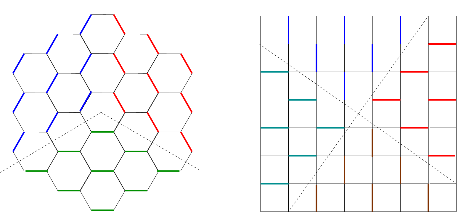
As is clear from Fig 2 (right panel), the simplest caricatures of vortices in the staggered valence bond solid order on the square lattice are indeed without any free spins at their core. In the staggered case, it is also possible to construct vortices with spins at their cores, but these are expected to cost more energy due to additional singlet formation cost associated with leaving one spin free in the core, as is clear from Fig 3 (right panel). This suggests that the transition would be strongly first order, which is consistent with recent numerical works [5, 6]. This should be contrasted with studies of very similar “” models on the square lattice, with the plaquette interactions chosen to favour columnar order[7]. Extensive numerical work on these models has led to the conclusion that the transition from Néel to columnar valence bond solid order is indeed a continuous transition, [9, 10, 8] although the critical point exhibits logarithmic violations of standard finite size scaling [8, 11]. These violations of scaling have also been interpreted as possible evidence of first order behaviour [12]. and versions of the same transition have also been studied [9, 13, 14] and found to be continuous in nature.

Here we focus on a related system on the honeycomb lattice: On the honeycomb lattice, the staggered ordering of near-neighbour valence bonds does not break lattice translation symmetry, but does break symmetry of three-fold lattice rotations. As is clear from Fig 2 (left panel), the simplest construction of elementary vortices in this valence-bond nematic order naturally yields vortices with spinless cores. Again, vortices with spinful cores are also possible, but are expected to cost more core-energy due to two reasons. First, forming a spinful vortex core shown in Fig 3 (left panel) involves the breaking of additional singlet bonds, and would cost an additional core energy of the order of the spin gap. At the same time, the spinless vortex core, shown in Fig. 2 (left panel), allows for dimer resonances on the core plaquette which is expected to lead to core energy lowering.
The transition between such a valence-bond nematic and a nearby antiferromagnetic phase on the honeycomb lattice is thus expected to be strongly first order based on our supposition above. Here we focus on a spin Hamiltonian with nearest neighbour exchange couplings that compete with four-spin interaction terms that stabilize a valence-bond nematic state. We study this system numerically by a projector Monte Carlo algorithm in the valence-bond basis, as well as analytically by spinwave and bond-operator expansions. Our numerics finds a strongly first order transition between a valence-bond nematic and a antiferromagnet, consistent with the intuitive picture outlined above. In addition, we use our approximate analytical calculations to provide a reasonable semi-quantitative account of our numerical results. We note that an exactly soluble model with such a valence bond nematic ground state has also been proposed recently.[15]
The remainder of the paper is organized as follows: In section II, we define the model studied, and describe the approximate analytical methods that we use for their study. In section III, we describe our numerical approach and summarize the results obtained. Finally, we conclude with a brief discussion in section IV.
II Model and analytical treatment
The honeycomb lattice staggered model Hamiltonian is defined as folows,
| (2) |
where the four spin plaquette operators are products of two bipartite singlet projectors acting on two parallel bonds of the hexagons in the honeycomb lattice (see Fig. 1(left panel)). This Hamiltonian can be written explicitly as a sum of two-spin and four-spin interactions as follows,
| (3) | |||||
| (4) | |||||
| (5) |
where denotes a sum over all hexagons of the lattice, denotes the -th spin on a hexagon, with - labelling the 6 sites clockwise around the hexagon, and = .
At a heuristic level, we expect that the term drives a transition to a valence bond nematic state with staggered ordering of near-neighbour singlet bonds, while the term favours a Neel state with spins on the -sublattice (-sublattice) of the honeycomb lattice aligned (anti-aligned) along a spontaneously chosen axis in spin space. A simple approximate description of the Néel phase is obtained by doing a standard spin wave analysis. On the other hand, to describe the valence-bond nematic, we use a description in terms of bond-operators that becomes very accurate in the limit of strong nematic order. By comparing the predictions for the ground state energy from these two approximate calculations, we also estimate the value of at which we expect a transition between the two phases.
II.1 Spin wave theory of the Neel state
In the Néel ordered phase of the JQ model defined above, let us assume we can decouple the four spin interactions as
| (6) |
where is the nearest neighbor spin correlation which is assumed to be the same on all neighboring bonds and which needs to be determined self-consistently. Such a decomposition can alternatively be obtained within a path integral formalism by using a Hubbard Stratonovich (HS) decoupling of the quartic spin operators followed by a static mean field theory of the HS field. In this case, the Hamiltonian reduces to the form
| (7) |
where we have defined , and is the number of unit cells on the lattice (the number of spins is ).
We treat this effective Hamiltonian using the standard spin wave theory by defining Holstein Primakoff bosons via and for sites on the A-sublattice and B-sublattice respectively. Retaining terms to quadratic order in the bosons leads to the Hamiltonian
| (8) |
where with and . Setting , we can diagonalize this Hamiltonian via a Bogoliubov transformation
| (9) |
where , , and . This yields the diagonalized Hamiltonian
| (10) |
with a ground state energy
| (11) |
Applying the Feynman-Hellman theorem to the mean field Hamiltonian, in Eq.7, yields
| (12) |
Eqns. (11) and (12), together, determine the ground state energy of this model in the Néel ordered phase. A feature of our mean-field spin-wave analysis is that is independent of . Numerically, we find within this spin wave approach which agrees with earlier spin wave results [16]. This value is quite close to the value, , deduced from a recent optimized valence bond trial wave function study [17] of the nearest neighbor Heisenberg model, and series expansion results [18] on the Heisenberg model which give . This spin wave result for must be used as input to compute the ground state energy per spin of the - model which is given by ; this is plotted in Fig.4. Within this approach, the ordered moment is also independent of , and is given by
| (13) |
and takes on a value , whereas series expansion studies of the nearest neighbor Heisenberg model [18] yield . In the next section, we will check to what extent the numerical results bear out our prediction of a nearly -independent value of in the Néel phase.
II.2 Bond operator theory of the staggered dimer state
In the other limit, when the term dominates over Hamiltonian at large has spontaneous staggered dimer order in the ground state, we can use a bond operator formalism to compute the ground state energy and correlations in this phase. We label the spins by their unit cell position and a sublattice index . In the staggered dimer state, let us assume that the spins at sites and in every unit cell form a singlet. This dimer pattern then spontaneously breaks the lattice rotational symmetry but leaves the translational symmetry intact. We define the singlet and triplet states on this pair of sites in terms of bond operators via
| (14) | |||||
| (15) | |||||
| (16) | |||||
| (17) |
where we must satisfy the constraint at each site. The spin operators can be rewritten in terms of the bond operators as
| (18) |
where . Assuming the staggered dimer state corresponds to a uniform singlet condensate, we can replace and . Furthermore, if the singlet condensate is robust, so that the dimer order is strong as observed in the QMC numerics, we expect the triplet density to be small and a Bogoliubov-type theory, where the triplet density plays the role of a small parameter, to be a reasonable starting point. Expanding out the Hamiltonian in terms of these bond operators, and retaining leading quadratic terms in the triplet operators, we find
| (19) | |||||
where is a chemical potential which serves to satisfy the constraint equation on average by fixing . Going to momentum space, the Hamiltonian takes the form
| (20) |
where
| (21) | |||||
| (22) | |||||
| (23) |
and the prime on the momentum sum indicates that we only sum over half the Brillouin zone (keeping states with for example). Diagonalizing this via a Bogoliubov transform
| (24) |
we find that the diagonal Hamiltonian takes the form
| (25) |
where . This leads to a ground state energy
| (26) |
This energy must be minimized with respect to once is determined by the number equation
| (27) |
which follows from demanding in order to satisfy the constraint relation .
Solving these equations numerically, we self-consistently determine and . Using these, we compute the ground state energy and excitation spectrum of the valence bond nematic state. As seen from Fig. 4, we find that the energy of this state lies below the antiferromagnetically ordered state for large , as we expect, but there is an energy level crossing at , so that the Néel state has lower energy at smaller . (Within the bond operator approach, we find that the triplons condense around which is well below the first order transition point.) Close to the transition, in the spin gapped phase, we find the spin-spin correlation on the dimerized bond to be which corresponds to nearly complete dimerization, so that this is a very strong first order transition. We next turn to a numerically exact quantum Monte Carlo study of this model.

III Numerical study
We use the valence bond projector Monte Carlo technique [19] to study various ground state properties of the staggered version model on honeycomb lattice as a function of coupling . Taking advantage of the improved loop-update technique developed in Ref. 20, we scan the phase diagram of this model for systems with upto sites. A Monte Carlo projection length of is used to ensure the convergence of observables to the ground state expectation values (we have checked the convergence by comparing with the results of exact diagonalization studies at small sizes). Also, to counter ergodicity problems in the Monte Carlo simulations in the valence bond nematic phase and in the vicinity of the first order transition, we employ many different Monte Carlo moves to update the bond and plaquette operators in a Monte Carlo configuration. These updates include attempts to reflect a plaquette operator about its diagonal bond (Fig.5a), to rotate the diagonal plaquette operators about a site (Fig.5b), to transform a plaquette operator into a bond operator by deleting a bond and vice versa (Fig.5c), and so on.

We find it convenient to define the valence bond nematic order parameter, , where denote the three nearest neighbor bond vectors of the honeycomb lattice. By monitoring the correlations of simultaneously with those of the spins, we are able to distinguish easily between the Neel antiferromagnet, and the rotation-symmetry breaking valence bond nematic. To do this we measure
| (28) |
where , and the sum over runs over all -sublattice sites of the lattice. We also define
| (29) |
where , and with being the linear dimension of the system and being the number of sites in the system. In the presence of long range antiferromagnetic order, the asymptotic large size limit of tends to a finite value, which equals the square of the staggered magnetisation
| (30) |
In the absence of long range antiferromagnetic order, we expect this quantity to vanish in the large size limit. Similarly, serves as a order parameter for long range valence bond nematic order.
III.1 Results for honeycomb lattice model

From our numerical study of these observables, we deduce that a transition from the Neel phase to the valence bond nematic phase takes place as is increased to the vicinity of . In this vicinity, there are clear first order jumps in both the order parameters as shown in Fig.6. At first sight, the data suggests that the transition point, as determined from the location of the jump, may have a tendency to drift with increasing system size. However, this is actually an artifact of the slowness of the code near the first order transition region at larger sizes, as is clear from an alternate more precise analysis which we now summarize. In this alternative approach, we determine the transition point by locating the kink in the plot of energy as function of tuning parameter at smaller sizes, where there are no such issue of slowness of the Monte Carlo update procedure used for calculating ground state properties. As shown in Fig. 7, the energy per site shows a linear behaviour, but with slopes of the line changing discontinuously near the transition. This can be understood as an avoided level crossing taking place at the first order transition point. Identifying the crossing point of these two linear extrapolations for the energy on is a convenient way to determine the transition point [5] with reasonable accuracy. Using this method, with data from three different system sizes and , we identify the first order transition to be at .

First order transitions are associated with two coexisting free energy minima corresponding to the two phases. This leads to the appearance of hysteresis effects in the vicinity of the transition for all but the most efficient Monte Carlo algorithms when a configuration from one of the phases is evolved by tuning the coupling constant across the critical value at finite rate (i.e without allowing for an extremely large number of equilibriation steps between each successive change of coupling constant). For example, starting with a configuration deep in the valence bond nematic phase, the system remains stuck in the metastable valence bond nematic state even when is reduced to less than and conversely, the system remains in the Neel phase upon ramping up beyond if one starts with a typical configuration obtained from the projection algorithm deep in the Neel phase. We present such a hysteresis plot for antiferromagnetic order parameter (Fig.8) near the transition to emphasize the first order nature of the transition.


Our QMC simulations also yield a characteristic double peaked order parameter histogram near as shown in Fig. 9. However, the ‘time’ (number of Monte Carlo steps) taken for the system to ‘tunnel’ between the two phases is extremely large, and it is therefore prohibitively expensive to perform runs that could encompass a large number of such tunneling events. As a result, it is not possible with our limited computational resources to obtain accurate estimates of the relative heights of the two peaks in the histogram.

Finally, we note that in a variant of staggered model on honeycomb lattice, where parallel bonds from neighbouring hexagons make up the plaquette interactions, we find that increasing fails to destroy AF order. For this model, as shown in Fig. 10, there is no hint of a transition even at large .
IV Discussion
We have thus studied an example of a transition between a Neel ordered antiferromagnet and a three-fold rotation symmetry breaking valence bond nematic on the honeycomb lattice. Our numerical results showed that the transition is strongly first order, consistent with the general scenario outlined in the introduction. The transition point obtained from our analytical considerations is at (), which is in reasonable agreement with the results of our QMC simulations, which give a strong first order transition at (). Furthermore, the nearly independent values of the staggered magnetization in the Néel phase, and of the nematic order in the staggered dimer state, are also consistent with our analytic considerations. These observations suggest that the bond operator approach provides a reasonable account of the dimer phase in situations where the kinetic fluctuations of dimers are not important in the vicinity of the transition. This appears to be different from the Néel to columnar dimer transition in the square lattice case where such singlet fluctuations appear to be important in driving the dimer order to zero at the quantum phase transition.[21]
V Acknowledgements
We acknowledge computational resources at TIFR, grant support (KD) from the Indian DST (DST SR/S2/RJN-25/2006), NSERC of Canada (AP), and an Early Researcher Award from the Government of Ontario (AP), and thank Arnab Sen and Anders Sandvik for useful discussions.
References
- [1] T. Senthil, L. Balents, S. Sachdev, A. Vishwanath, and M. P. A. Fisher, Phys. Rev. B 70, 144407 (2004).
- [2] T. Senthil, A. Vishwanath, L. Balents, S. Sachdev, and M. P. A. Fisher, Science 303, 1490 (2004).
- [3] A. Mulder, R. Ganesh, L. Capriotti, and A. Paramekanti, Phys. Rev. B 81, 214419 (2010).
- [4] M. Levin, and T. Senthil, Phys. Rev. B 70, 220403 (2004).
- [5] A. Sen, and A. W. Sandvik, arXiv:1009.0691.
- [6] A. Banerjee, Ph.D thesis, unpublished.
- [7] A. W. Sandvik, Phys. Rev. Lett. 98, 227202 (2007).
- [8] A. W. Sandvik, Phys. Rev. Lett. 104, 177201 (2010).
- [9] J. Lou, A. W. Sandvik, and N. Kawashima, Phys. Rev. B 80, 180414 (2009)
- [10] R. G. Melko and R. K. Kaul, Phys. Rev. Lett. 100, 017203 (2008)
- [11] A. Banerjee, K. Damle, and F. Alet, Phys. Rev. B 82, 155139 (2010).
- [12] F. J. Jiang, M. Nyfeler, S. Chandrasekharan, and U. J. Wiese, J. Stat. Mech.: Theory Exp. (2008) P02009.
- [13] R. K. Kaul, arXiv:1010.1937, unpublished (2010).
- [14] A. Banerjee, K. Damle, and F. Alet, arXiv:1012:3691.
- [15] R. Kumar, D. Kumar, B. Kumar, Phys. Rev. B 80, 214428 (2009).
- [16] J. D. Reger, J. A. Riera, and A. P. Young, J. Phys. C 1, 1855 (1989).
- [17] Z. Nourbakhsh, F. Shahbazi, S. A. Jafari, and G. Baskaran, J. Phys. Soc. Jpn. 78, 054701 (2009).
- [18] J. Oitmaa, C. J. Hamer. and Z. Weihong, Phys. Rev. B45, 9834 (1992).
- [19] A. W. Sandvik, Phys. Rev. Lett. 95, 207203 (2005).
- [20] A. W. Sandvik, and H. G. Evertz, Phys. Rev. B 82, 024407 (2010).
- [21] V. N. Kotov, D. X. Yao, A. H. Castro-Neto, D. K. Campbell, Phys. Rev. B 80, 174403 (2009).