August 24, 2026
UMD-PP-10-015
Using to Distinguish Dark Matter Stabilization Symmetries
Kaustubh Agashe, Doojin Kim, Devin G. E. Walker and Lijun Zhu
1Maryland Center for Fundamental Physics, Department of Physics, University of Maryland, College Park, Maryland 20742, U. S. A.
and
2Center for the Fundamental Laws of Nature, Jefferson Physical Laboratory, Harvard University, Cambridge, Massachusetts 02138, U. S. A.
Abstract
We examine the potential of using colliders to distinguish models with parity () stabilized dark matter (DM) from models in which the DM is stabilized by other symmetries, taking the latter to be a symmetry for illustration. The key observation is that a heavier mother particle charged under a stabilization symmetry can decay into one or two DM particles along with Standard Model (SM) particles. This can be contrasted with the decay of a mother particle charged under a parity symmetry; typically, only one DM particle appears in the decay chain. The arXiv:1003.0899 studied the distributions of visible invariant mass from the decay of a single such mother particle in order to highlight the resulting distinctive signatures of symmetry versus parity symmetry stabilized dark matter candidates. We now describe a complementary study which focuses on decay chains of the two mother particles which are necessarily present in these events. We also include in our analysis the missing energy/momentum in the event. For the symmetry stabilized mothers, the resulting inclusive final state can have two, three or four DM particles. In contrast, models with symmetry can have only two. We show that the shapes and edges of the distribution of -type variables, along with ratio of the visible momentum/energy on the two sides of the event, are powerful in distinguishing these different scenarios. Finally we conclude by outlining future work which focuses on reducing combinatoric ambiguities from reconstructing multi-jet events. Increasing the reconstruction efficiency can allow better reconstruction of events with two or three dark matter candidates in the final state.
1 Introduction
A stable weakly interacting massive particle (WIMP) – with a mass also of order the weak scale – is a well-motivated candidate for dark matter (DM) in the Universe since it approximately has the correct relic density upon thermal freeze-out [1]. Such a particle also often arises in extensions of the Standard Model (SM), especially those motivated by solutions to the Planck-weak hierarchy problem of the SM. Finally, if the WIMP is a part of an extension of the SM, then it is likely to have (weak) interactions with SM particles. Hence, the WIMP paradigm can be tested via non-gravitational methods, for example, direct/indirect detection of cosmic DM or production of the DM at colliders. The latter is our interest here.
The collider searches of the DM paradigm typically involve producing a heavier particle charged under the same symmetry which stabilizes the DM. Such a “mother” particle must decay to SM particles and DM, manifesting as missing energy, along with a SM final state. Reconstructing the decay chains leading to such events will enable us to determine the masses of the DM and the mother particles; it is advantageous to do this in a model-independent manner. A tremendous amount of effort has been put-in into such a research program, especially at the CERN Large Hadron Collider (LHC), see, for example [2, 3, 4, 5, 6, 7, 8, 9, 10, 11, 12, 13, 14, 15, 16, 17, 18, 19, 20, 21, 22]. See also [23] for a review. Most of this work still assumes that a /parity symmetry stabilizes the DM (henceforth called models). This is partly because there are several models with such a symmetry [25, 26, 27, 28, 29]. However, while might be the simplest possibility for such a symmetry, it is by no means the only one [30, 33, 32, 34]. So, in previous work [31, 36], the program of instead determining the DM stabilization symmetry from collider data was started. We focused on how to distinguish a DM stabilization symmetry (henceforth called a model) from a model11 1 See reference [35] for how calculation of relic density and indirect detection might be modified in a model vs. a model. Also see reference [31] for a collider study of non- models, but with decays of mother particles into DM occurring outside the detector vs. the case of such decays taking place inside the detector studied here and in reference [36].. We have focused on models for simplicity and definiteness. However, we emphasize our techniques in this and in previous papers [31, 36] can be generalized to distinguish most other DM stabilization symmetries from parity symmetry stabilized DM.
The basic idea behind distinguishing from models is that a
- •
single mother charged under a symmetry is allowed (based simply on the symmetry) to decay into one or two DM candidates.
This is to be contrasted with the fact that mother particles charged under a symmetry have only one DM candidate in the final state22 2 In both and models, a mother can decay into three DM particles, but we will not consider this possibility here for simplicity and since it is expected to be phase-space suppressed compared to the other possibilities.. As discussed in reference [36], decays of a single -charged mother particle generate a “double edge” in the invariant mass distribution of the visible (SM) particles. This is with the condition that the intermediate particles in the decay chains are off-shell and that the decay chains with one and two DM contain identical SM particles. For the case of on-shell intermediate particles, it was shown in [36] that this invariant mass distribution has a “cusp” for certain decay topology (with two DM) of a mother particle. In all, [36] focused on new features in observables from a single decay chain only.
In this work we consider the total inclusive event in order to glean even more information, recalling that there must be two such mother particles present. For example, consider the case where there is only one visible (SM) particle in the decay chain of a mother particle. Constructing the invariant mass of the visible particle of this decay chain, as per the analysis of [36], is not very useful for the purpose of reconstructing the mass of the mother particle: one might have to resort to including information about the invisible particle(s) in the same decay chain. Since we can only measure the total missing transverse momentum in the event which is shared between invisible particles from two mothers, we must use measurements from both sides. An option is to use “”-type observables/variables [2, 3, 4, 5, 6, 7, 8, 9, 10, 11, 12, 13, 14, 15, 16] Another case where one of the analyses of reference [36] (based on single mother decay) might not work is when the visible/SM particles in the decay chains with one and two DM (of course for model) are not identical (even if they are more than one). Thus, one does not obtain a double edge for the case of intermediate particles in the decay chains being off-shell.
With the above motivations in mind, in this paper,
- •
we develop techniques for distinguishing models from models using information from both mother decays and the missing (in addition to visible) energy/momentum in an event.
We especially study the above cases where the techniques of reference [36] might not work – in this sense, our present work is complementary to that of reference [36].
- •
We show that shapes and edges of these distributions, along with the ratio of visible momentum/energy on the two sides of the event, act as powerful discriminants between and models (including the case of a neutrino, i.e., massless invisible particle – in addition to DM, in the final state for models).
An outline of this paper is as follows: In the next section, we begin with a review of variable in models. We present some important formulas such as the location of maximum value of the distribution, and discuss some interesting features such as a “kink” in the maximum as a function of the “trial” DM mass in the case where more than one visible particle is involved in each decay chain. In Sec. 3 we move on to the variable in models. We define three different event types arising in models based on the number of dark matter particles in the final state and provide their corresponding theoretical predictions of the maximum . In particular, we discuss the conditions to have a kink in maximum as a function of trial DM mass for the cases where there exist more than two DM particles in the final state: such situations do not arise in models. We further show some simulation results for distributions for the new types of events in models and discuss some notable features to be used for distinguishing models from models.
In the following two sections, we provide detailed applications of our results of the previous two sections for distinguishing from models. First we consider the easier case where the decay chain with one DM contains visible/SM particle(s) which are not identical to the ones in the two DM decay chain mentioned above (in models). Based on the theoretical considerations given in Secs. 2 and 3, we provide ways of distinguishing models from models, as well as measuring the mother and DM masses. We do it for both the case of one visible/SM particle in the two decay chains and more than one visible/SM particle case. In the next section we deal with the case where one DM and two DM decay chains contain identical visible/SM particle(s), and discuss additional techniques required in this case to distinguish and models. In all of the examples above, we make the simplifying assumption that the intermediate particles in the decay chain are off-shell, i.e., they are heavier than the mass of their mother particle. In section 6, we briefly mention some aspects of the case of intermediate particles being on-shell. We next conclude and show details of some of the calculations in the Appendix.
2 A Review of for Models
For simplicity, in this paper
- •
we consider pair-production of a single type of mother particle which is charged under the DM stabilization symmetry.
We also assume that the total transverse momentum of the two mother particles produced in an event is zero, for example, we neglect any initial/final state radiation. In models, each such mother decays into SM/visible particle(s) and one DM/invisible particle33 3 We assume that there is only one type of DM particle in this (and similarly the ) model so that the invisible/DM particles in each decay chain are identical.. Furthermore, it is assumed
- •
we know which visible particle(s) originate from which decay chain.44 4 Of course, for models, we do not know which decay chain emits one or two DM particles. For example, if the pair-produced mother particles are boosted sufficiently, their decay products are likely to be collimated so that the visible particles coming from the same decay chain are detected in the same hemisphere in the collider. For alternate methods of determining the correct assignment of visible particles to the two decay chains, see reference [37] and section 6.3.
The variable [2, 3] is a generalization of the transverse mass55 5 Of course, the usual transverse mass assumes only a single mother particle. to this case. Specifically, for each event, it is defined to be a minimization of the maximum of the two transverse masses in each decay chain under the constraint that the sum of all the transverse momenta of the visible and invisible particles vanishes [2, 3]:
| (1) |
where denote the vector sum of visible transverse momenta and denote the transverse momentum of the invisible particle in the ith decay chain (): the minimization is performed over the latter momenta. is the usual transverse mass:
| (2) |
where and are (respectively) the transverse energy and transverse mass formed by all visible particles belonging to the same decay chain. The variables with a tilde represent the corresponding quantities formed by the invisible particle in the same decay chain. Note that the mass of the invisible particle should be regarded as a unknown/free parameter because we are not aware of it in advance, and henceforth we call it “trial” DM mass. In this sense should be considered to be a function of the trial DM mass , and its maximum value among many events (which will be used extensively in the following) is defined as
| (3) |
Obviously is also a function of the trial DM mass (see App. A for details). An important result to be noted is that if there are a sufficient number of events and the actual DM mass is substituted into , then the above-given becomes the actual mass of the pair-produced mother particles [2, 3]:
| (4) |
where and indicate the true masses of mother and DM, respectively.
In order to see how this analysis is applied to realistic situations, we first take the case where there exists a single visible/SM particle in each decay chain, and then move on to the case where there exists more than one visible/SM particle in each decay chain. A similar analysis can be done for the mixed case, i.e., one visible particle on one side and more than one on the other.
2.1 One Visible/SM Particle in Each Decay Chain
In this case the upper edge in distribution is obtained by “balanced” [2, 3, 4] solution (see App. A for details).
| (5) |
Here (and henceforth)
- •
we assume that all visible particles are massless for simplicity.
As mentioned earlier, the above-given upper edge is a function of the trial DM mass and one can see that it reduces to the true mother mass with equal to the true DM mass .

The left panel of Fig. 1 shows the above theoretical prediction for the location of maximum for models as a function of the trial mass . We used 400 GeV and 100 GeV as mother and DM particle masses. As expected from Eq. (5), the curve in the figure “smoothly” increases with (cf. the following section), and that the value corresponding to (here 100 GeV) is the same as the true mother particle mass (here 400 GeV: see the black dotted lines).
2.2 More than One Visible/SM Particle in Each Decay Chain
Once there exists more than one visible particle per decay chain, another type of solution to , denoted by “unbalanced” [2, 3, 4], arises. If
- •
we assume that the intermediate particles in the decay chains are off-shell, i.e., heavier than their mother particles
(as we will for most of this paper), then the balanced solution in this case is still given by Eq. (5), and the unbalanced solution is as follows66 6 Of course, in general, one can find the expressions for both the balanced and the unbalanced solutions in the case of on-shell intermediate particles [4].:
| (6) |
Hence the overall upper edge in the distribution is determined by a “competition” between balanced and unbalanced solutions:
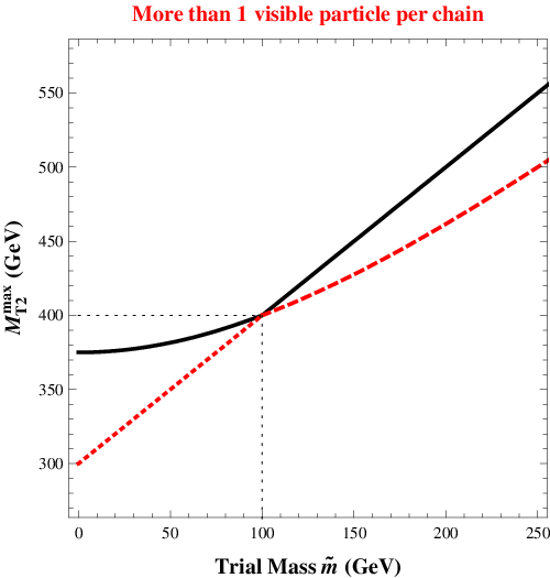
Note that the shows different functional behaviors depending on the relative size of the trial DM mass to the true DM mass. As a result, is no longer smoothly increasing with in contrast to the case with one visible/SM per decay chain. Instead, there arises a “kink” at the location of the actual DM mass, with the corresponding being the actual mother mass [4]77 7 A similar kink also appears for the case of one visible particle in each decay chain if the total transverse momentum of the two mother particles is non-zero, for example, in the presence of initial/final state radiation (see [5]), but (as mentioned earlier) we neglect this possibility for simplicity.. This is illustrated in the right panel of Fig. 1 where the upper edges for the two possible types of solutions and are shown by a straight line (i.e., the dotted line, which extends into the right-hand part of the solid line) and a dashed curve (which extends into the left-hand part of the solid curve), respectively. The upper edge in the distribution is given by the larger of these two values, i.e., the black solid curve, and shows a kink (indicated by the black dotted lines), at GeV and GeV (as expected).
3 for Models
To begin with, we would like to reiterate some of the relevant features of symmetry in order to avoid any possible confusion later. Under the symmetry, a particle/field transforms as
| (11) |
where (i.e., neutral) or +1, +2. Suppose the lightest of the charged particles (labeled ) has charge (similar argument can be made for charge ). Clearly, its anti-particle () has (a different) charge (which is equivalent to ) and has the same mass as . Then, solely based on symmetry considerations, all other (heavier) -charged particles can decay into this lightest -charged particle or its anti-particle (in addition to -neutral particles, including SM particles). To be explicit, a heavier -charged particle with charge can decay into either (single) or two ’s (and -neutral particles). Taking the CP conjugate of the preceding statement, we see that a heavier -charged particle with the other type of charge, namely , is allowed to decay into two ’s or single . Of course, or cannot decay and thus is the (single) DM candidate in this theory. We will denote this DM particle and its anti-particle by DM and , respectively, although we do not make this distinction in the text since DM and anti-DM particles are still degenerate.88 8 Of course, which of the two particles is denoted anti-DM is a matter of convention. Also, as a corollary, the DM particle should be Dirac fermion or complex scalar in a model.
According to the above-given argument, for models, each mother particle can emit either one or two DM particles so that there exist two, three, or four DM particles in the final state (for pair-production of mothers) while there are only two DM particles for models. We therefore expect richer structures in the distribution for models. Here
- •
we take as an ansatz only a single DM particle in each decay chain for the sole purpose of defining , even if there could be two DM particles in either or both of the two decay chains.
We do so for the following two reasons. First, in the real collider experiment, there is (a priori) no clear information on the number of invisible particles involved in the decay process of interest so that each individual decay chain with only one DM is a natural (starting) assumption. Moreover, one can naturally expect (and we will show) that decay events from models will show different features in the analysis compared with those for models. Therefore, starting with a assumption and deriving a “contradiction” in the analysis, we can distinguish models from ones (which is our primary goal here). In this context, we call such an analysis imposing one-DM-per-chain assumption the “naive” analysis.
For a more systematic consideration let us define the three different events having different numbers of (a single type of) DM particles as , , and -type, respectively, i.e., each subscript on simply implies the total number of DM particles in the final state: see Fig. 2, where SM1, 2 denote the visible/SM final states (irrespective of the actual number of particles in the state) in the decay chains with one and two DM (respectively)99 9 These two SM final states might not or might be identical: we will return to these two possibilities in the next two sections (respectively).. Here the red dashed lines denote any particles charged under dark matter stabilization symmetry (in this section symmetry) while the black solid lines/arrows denote any visible/SM particles. One should note that type events represent the case with 2 DM particles in each decay chain. Also, both decay chains (with one and two DM) might not exist for a specific mother so that all three types of events might not occur. Like in models, we start with the case with one visible/SM particle in each decay chain, and we consider the case with more than one visible/SM particle in each decay chain in the following subsection. While doing so, we see how the analysis applied to models contrasts with models.


3.1 One Visible/SM Particle in Each Decay Chain
In this case the upper edge in the (naive) distribution is determined only by the balanced solution like models, and the analytic expressions for the three type events are given as follows (see App. A for details):
| (12) | |||
| (13) | |||
| (14) |
As a reminder, the events with , and represent events with two, three and four dark matter candidates. Note that Eq. (12) has the same form as Eq. (5) in models because type events also contain two DM particles in the final state (just like models) whereas the other two types of events do not appear in models so that the corresponding Eqs. (13) and (14) (and similar ones later) are new/do not appear in previous literature. Substituting in Eq. (12) gives the true mother mass for the value of (as expected), but the other two equations give a combination of the true mother and DM masses rather than the true mother mass. Actually, this is not surprising because we have used the naive variable for the -type events in models, whereas the actual physics is different from the physics under which our variable is defined. For example, for type events there is an asymmetry between the final states of the two decay chains, which is caused by adding one more DM to either of the two decay chains. For type events, even though the two decay chains have symmetric final states, the “effective” DM mass is twice the true DM mass so that the true mother mass (for the value of ) is in fact obtained by setting instead as clearly seen from Eq. (14).
All of the theoretical predictions mentioned above are demonstrated in the left panel of Fig. 3.


Again, we used 400 GeV and 100 GeV as mother and DM masses. The black solid, the red dashed, and the blue dot-dashed curves represent the theoretical expectations of for , , and type events, respectively (the curve for -type events is of course the same as in right-hand side of Fig. 1). As discussed above, the for type events corresponds to the true mass of the mother particle (here 400 GeV) with the trial DM mass equal to the true DM mass (here 100 GeV) whereas type events do it for twice the DM mass (here 200 GeV), as shown by the dotted/black lines.
In addition, there are a couple of features to be noted; there is no kink arising in the curves for -type events just like the case of a single visible particle per decay chain in models (or an -type event in models). Second for any given , the values form a hierarchy of
| (15) |
3.2 More than One Visible/SM Particle in Each Decay Chain
Once more visible particle(s) are added in each decay chain, one could naturally expect that a kink appears like in models. The reason is that, just like for models, the maximum unbalanced solutions take part in determining the overall upper edge in the distribution together with the balanced solutions. It turns out, however, that this expectation is true only for and type events which we discuss to begin with. Again, assuming the intermediate particles are off-shell the maximum values of the balanced solutions for and type events are simply given (as for the one visible particle case) by Eqs. (12) and (14), respectively, and those of the unbalanced solutions are given as follows:
| (16) | |||||
| (17) |
Here Eq. (16) is of exactly the same form as Eq. (6) due to the similarity between the decay structures for models and type events while Eq. (17) for -type events is relevant only for models, i.e., it is not present in models. More quantitatively, the above-given two equations differ by for any given because one more DM particle is emitted in both decay chains for type events compared with type events (see Eqs. (77) and (103) in App. A).
As mentioned for models, the maximum values are given by the larger of the balanced and unbalanced solutions: for type events as in Eq. (2.2), and for type events by
Note that there is also a kink for -type events as seen from Eq. (3.2), but at (i.e., not ), because the effective DM mass for is given by .
The right panel of Fig. 3 illustrates the above theoretical considerations for and type events (of course the curve for -type events is the same as the right-hand side of Fig. 1). As before, the two straight dotted lines which extend into the right-hand parts of the solid lines indicate the maximum values of the unbalanced solutions while the two dashed curves which extend into left-hand parts of the solid curve indicate the maximum values of the balanced solutions. The actual upper edge in the distribution for any is given by the black (for type events) or blue (for type events) solid curves. Identifying the location of the kink in -type events and its corresponding enables us to determine the masses of mother and DM particles separately (just like in models). The figure also shows the kink for -type events, but located at GeV (i.e., , as expected) and GeV. This observation can be used as a cross-check for the determination of and based on -type events (again, this feature is new in models relative to ).
On the other hand, as far as type events (which are absent in models) are concerned, whether or not there exists a kink depends on the mass hierarchy between mother and DM particles (see App. B for details). Again, assuming off-shell intermediate particles the maximum balanced solution is simply given by Eq. (13) (just like the case of one visible particle per decay chain), whereas the maximum unbalanced solution has the same form as that for type events because one of the two decay chains still emits a single DM particle in the final state (see Eqs. (77) and (103) in App. A).
| (22) |


If the ratio of the DM mass to the mother mass is larger than , it turns out that the maximum unbalanced solution given in Eq. (22) is always bigger than the maximum balanced solution given in Eq. (13) so that
| (23) |
The left panel of Fig. 4 clearly confirms our expectation (based on above equation) that there occurs no kink in the upper edge of as a function of the trial DM mass, i.e., the upper edge in the distribution is always determined by the unbalanced solution (black solid line), not by the balanced solution (red dashed curve). Here we adopted GeV and GeV, and thus the ratio between them is obviously larger than .
On the other hand, once the ratio of DM to mother mass is smaller than , the competition between the balanced and the unbalanced solutions results in
| (28) | |||||
where
| (29) |
We see that there is a kink at . Here is not simply the true DM mass but it is given by a combination of the true mother and DM masses (in fact, it is smaller than the true DM mass), which is clearly different from that in models. The functional behavior of for this case is shown in the right panel of Fig. 4. Here we took GeV which makes the ratio smaller than . As before, the maximum for the balanced and unbalanced solutions are shown by the dashed and dotted curves (which extend into the black solid curve to the RHS and LHS). The final maximum is given by the larger of these two solutions (black solid curve) which clearly shows a kink at a value of which is different from the actual DM mass GeV (shown by the vertical black dotted line) as expected based on above discussion. Of course, we can still evaluate the masses of mother and DM particles (using -type events only) by obtaining and from the above analysis, substituting them into Eqs. (28) and (29), and solving those two equations about and .
Next, let us investigate the hierarchy among the three values for , , and type events. Although a bit more complicated than the one visible particle case, it is nonetheless straightforward to derive this hierarchy based on above equations, We have a following hierarchy among the values for the three types (cf. the one visible particle case shown in Eq. (15)):


3.3 Shapes of Distributions
Before closing the present section, let us examine the shape of the distributions for cases. For this purpose we simulated events using MadGraph/MadEvent [38]. Here and in sections 5.1.1 and 5.1.2, we make the following assumptions (mostly for simplicity): (a) effects of spin correlations are neglected in both production and decay of mother particles, i.e., we assumed scalar particles only in our simulations,; (b) the beam is proton-proton with 14 TeV total energy in the center of mass frame (motivated by the LHC parameters); (c) the non-colored (scalar) mother particles are pair-produced via s-channel exchange (of another scalar particle); and finally (d) only the relative values of the number of events (on vertical scale) are meaningful, i.e. only the shape of the distributions is the robust aspect of our analysis.
For all the simulations in this section, the masses of mother and DM particles used in the (toy) model are 400 GeV and 150 GeV, respectively, we took a single visible particle per decay chain for simplicity and chose a small trial DM mass (here 6 GeV) for the purpose of illustration. The upper left panel of Fig. 5 demonstrates the distribution for type events. Obviously, this is similar to the distribution for events in models [2, 3, 4], which is not surprising because type events also have only two dark matter particles in the final state like . The (naive) distribution for type events illustrated in the upper right panel of Fig. 5 has two notable features. As expected from the analytic expressions given before, first of all, the location of the upper edge is clearly lower than that for type events (or for models). Secondly, the shape of distribution for type events shows a long tail near the upper edge compared with type events (which have relatively sharp upper edge): this is because more physical constraints (e.g., rapidity) between decay products should be satisfied in type events in order that they form a kinematic configuration to give maximum , thereby reducing the corresponding number of events near .
This feature of a (relatively) long tail is also true for a special case in models with three invisible particles in the full event one of which is a (massless) SM neutrino, i.e., with one DM in one decay chain, but one DM and a neutrino in the other (henceforth we call it events)1010 10 distributions for such events have been studied in [3] and in [24].. The bottom panel of Fig. 5 demonstrates the distribution for events, assuming intermediate particles are off-shell 1111 11 As for the events with three (or more) DM, we assume here that there is a single (massive) invisible particle in each decay chain for the purpose of defining .. At the upper edge it shows a tail which is longer than that for type events (or neutrino-less events in models), but which is not as long as that for type events1212 12 This feature of a long tail in -type events is valid even for the case of more than one visible particle in each decay chain.. Such a shape is not surprising because the additional invisible particle (neutrino) in vs. -type events is massless so that events can be understood as a transitional type between and type events. However, it is crucial to note that the location of the upper edge for the events is the same as that for usual (i.e., neutrino-less) events in models with only a single massive invisible particle per decay chain, because the effective DM mass in former decay chains is also . We can therefore distinguish the events from the -type events in models by observing the location of the upper edge: the latter events will have a smaller edge.
4 Applications: Non-Identical Visible Particles in the Two Decay Chains
Next, we apply the theoretical observations on the technique for and models, which are described in the previous sections, for distinguishing models from ones in some specific cases. Like in the previous sections, we assume (for simplicity) pair-produced (same) mother particles and that all visible particles are massless and use the naive analysis for all events. As mentioned earlier, in models each mother particle can decay into either one or two dark matter particles along with visible/SM particle(s). Here,
- •
we consider a mother particle in a model for which both these decay chains (with one and two DM, respectively) exist.
Similarly, in models the mother particles can only decay into a single dark matter particle along with visible/SM particle(s). Here, we assume two such decay chains for a -mother which have the same visible final states as the above two -mother decay chains (respectively). The idea behind this choice is that such a model could easily fake a one (at least based on the identity of the visible states). This motivates us to distinguish these two types of DM stabilization symmetry using the variable.
For later convenience, we divide the discussion into two cases based on whether or not the visible state in the decay chain with one DM is identical to the one in the decay chain with two DM in the model. We begin with the case where the SM final states in the two decay chains are not identical (this includes the case of partial overlap between these final states). Following the notation of previous section, let us denote SM1, 2 to be these SM final state particles – whether they consist of one or more SM particles – in the two decay chains. And, for the model, assume that SM1 comes with one DM particle and SM2 is associated with two DM particles.1313 13 Since a model does not allow two DM particles in each decay chain, SM1 and SM2 are both emitted with only one DM in the final state in this model. We thus have three distinct (based simply on identity of visible states) types of events in both the and models, denoted by SM11, i.e., SM1 on each side/from each mother and similarly SM12, 22. Clearly, for models, these three types of events correspond (respectively) to -type events mentioned in the previous section and shown in Fig. 2 (with SM1 SM2). Hence, we can apply the formulas for the theoretical predictions of for , , and type events derived in the previous section to the SM11, 12, 22 events.
4.1 One Visible/SM Particle in Each Decay Chain
As a further subcase, we assume that SM1,2 consist of only one particle. Clearly, the upper edges of the variable for SM11, SM12, and SM22 are given by Eqs. (12), (13), and (14), respectively. As is obviously seen from the left panel of Fig. 3 or equivalently Eq. (15), the location of the upper edge for SM12 or SM22 is lower (for all trial DM mass : cf. the case of more than one visible particles below) than that for SM11 (for the same mother and DM masses). In contrast, in the model we have the same expression for given by Eq. (5) for all of SM11, SM12, and SM22 because they all involve two DM particles in the final state. Thus,
- •
different edges for the SM11, 12, 22 events (in particular, larger for SM11) can be evidence for models, i.e., they provide discrimination between and models1414 14 unless multiple mother particles in the models decay into the identical final state..
We can be further quantitative:
- •
for models we can measure the masses of mother and DM separately as follows (in spite of absence of kink in left panel of Fig. 3).
Note that the theoretical formulas for in Eq. (12) through Eq. (14) – considered as a function of trial mass – have a structure of where is a constant. So, the idea is to choose an arbitrary trial mass, then calculate the corresponding from the experimental data and thus determine the above-defined . Also, in our specific case where visible particles are assumed massless, the theoretical formula for each is written only in terms of the mother mass and the DM mass:
| (34) | |||||
| (35) |
Solving the above-given two equations, we obtain both mother and DM masses 1515 15 The upper edge from SM22 provides redundant information, but of course can be a cross-check.:
| (36) | |||||
| (37) |
This situation is somewhat like the double-edge signal for single mother decay studied in reference [36], where it was again possible to obtain mother and DM masses from the two edges in invariant mass distribution of visible/SM final state.
On the other hand, for models, we obtain only a combination of mother and DM masses from the (single) measurement of , given by
| (38) |
and thus it is not possible to determine mother and DM masses separately.
4.2 More than One Visible/SM Particle in Each Decay Chain
In this case, there is more interesting behavior of than the case of one visible particle per chain 1616 16 In the SM12 events, the endpoints of the visible invariant mass distributions for the two sides of the event/decay chains will be different in models, i.e., in -type events (vs. being the same in models), already providing a discrimination between the two types of models [36]. However, developing another technique for distinguishing from models based on can still be useful.. The upper edges of for SM11, 12, 22 events are now obviously given by Eqs. (2.2), (23), (28) and (3.2), respectively. As discussed in Eq. (3.2), the upper edge for SM12 is the same as that for SM11 (cf. one visible particle case above) for , but is lower for than that for SM11. And, the upper edge for SM22 events is always lower than SM11. This fact enables us to distinguish models from ones because in models the upper edges for SM11, 12, 22 coincide for all (just like the case with one visible particle in each decay chain).
Moreover, there occurs a kink in the upper edge of as a function of the trial DM mass as discussed in the previous sections. Because of the existence of this kink structure, SM11 itself is sufficient for the purpose of determining mother and DM masses (again, unlike one visible case): the trial mass which gives rise to a kink is the true DM mass and its corresponding is the true mother mass. (Of course this is how one can measure the masses of mother and DM particles separately even in models.) Such a direct measurement of mother and DM masses leads us to
- •
a prediction (cf. one visible case) on the location of the upper edges for the other two types of events, namely SM12 and SM22, a confirmation of which can provide evidence for symmetry as underlying physics1717 17 We can also predict (and then verify) location of kink in SM22 events. Alternatively, we can use kink in SM22, i.e., -type events to determine the mother and DM masses and then make predictions..
For SM12, i.e., -type events, actually, there are more interesting aspects of the kink structure in due to the dependence on the ratio of DM and mother masses: as discussed in Sec. 3, the critical ratio is given by
| (39) |
The kink is present only when the ratio of DM and mother masses is less than the above-given critical ratio. In this case, the kink location can be predicted by substituting mother and DM masses measured from the kink in SM11 into Eq. (29) so that it can provide a further verification for symmetry1818 18 Alternatively, this kink can be used to determine mother and DM masses, which are then used to predict edges/kinks in other events..
Finally, note that another way to distinguish from models in this case was discussed in [36]. The idea is to use SM12, i.e., -type, events in models, where edges in invariant mass distributions of visible particles on each side are different, i.e., and (vs. the two edges being the same for models).
4.3 Signal Fakes by an (Effective) 2nd DM Particle
In the two previous sections we have focused on decay processes with a single type of DM particle in the final state (for both and models). The crucial observation for the sake of discriminating from models is that models have more event-topologies (i.e., , , and type events with different upper edges in distributions) than the case of (which has a single upper edge), regardless of the number of visible/SM particles in each decay chain. In turn, this contrasting feature is due to the different possibilities in each decay chain in models, i.e., presence of one or two DM (unlike only one DM in case).
However, models can also acquire such different possibilities for decay chains (and thus fake signals in the analysis) if we assume that there is a second DM (obviously -odd) particle (with larger mass) denoted by DM′ into which the -mother can decay, i.e., there are actually two (absolutely) stable DM particles in a model [40]. Clearly, even with only one DM in a model, a similar effect can arise from a mother decaying into an (-odd) on-shell color/electrically neutral particle which decays (into DM particle and SM, possibly visible), but outside the detector (i.e., there exists a -odd particle – other than the DM – which is stable and invisible as far as the detector is concerned). Another related possibility is that there is a -odd (on-shell) neutral particle which decays inside the detector, but invisibly, i.e., into DM and invisible SM, for example, neutrino. A classic example of the last type is found in supersymmetry where sneutrino decaying into neutrino and lightest neutralino (which is assumed to be the lightest supersymmetric particle, i.e., DM). Even in the latter two cases, there is “effectively” (i.e., as far as the collider analysis is concerned) a second “DM” and so we will denote it also by DM′. In particular, in the last case mentioned above, i.e., even if there is an (on-shell) neutral particle decaying invisibly inside detector, the theoretical prediction of the variable is the same as with a DM′ of the same mass as this neutral mother particle.
Here, we note that the reference [10] has studied such (asymmetric) events using an type analysis, in particular, variants of the usual variable have been developed. As before, we will instead apply the naive/usual variable, i.e., assume (again, just for the purpose of constructing ) that there is a single and same DM in both decay chains.
In more detail, the above case in models gives rise to “-faking” signals is as follows. As before, consider pair production of a single mother such that decay chains with DM and DM′ are both allowed. Consequently, we obtain three distinct decay topologies for the full event: two DM, one DM and one DM′ and two DM′. We will denote these three types of events by , , and since they obviously resemble (and thus can fake) , , and type events being found in models, respectively. In particular, we can expect three different upper edges for in , , and -type events1919 19 An extreme case is when DM′ is massless, for example, SM neutrino. However, in this case, as mentioned in section 3.3, the upper edges for (denoted by event in section 3.3) and -type events will be same as for -type events. Thus this case can be easily distinguished from models.. Explicitly, the maximum balanced solutions for them (for both the cases with one visible particle per decay chain and more than one visible particle per decay chain) are simply given as follows:
| (40) | |||
| (41) | |||
| (42) |
and the maximum unbalanced solutions (only for the case with more than one visible particle per decay chain) are given as follows:
| (43) | |||||
| (44) | |||||
| (45) |
Here denotes the mass of the second DM-like particle. Again, all three types actually contain two DM/DM-like particles, i.e., the subscripts on do not imply the number of DM particles in a full decay chain but rather indicate the respective topologies in models which they fake. Note that if we set , then the above edges are exactly the ones in a model (see Eqs. (12) through (14) and Eqs. (16), (17), and (22) from previous sections. This feature is as expected since for -type events (in models) which are at the edge of the respective distributions, the two DM from the same mother are collinear so that their invariant mass is , i.e., the decay chain with two DM effectively has single DM of this mass as far as -edge is concerned.
Despite the fact that such events with a second DM-like particle can introduce three decay topologies, we can still differentiate and models. However, the strategies to be applied depend on the number/identity of visible particles in each decay chain. In this section, we consider the case where the visible particles in the decay chain with DM (denoted by SM1, following the notation used earlier) are different than the visible particles (denoted by SM2) in decay chain with DM′ in the model or two DM (in the model). Thus, the three types of events SM11, SM12 and SM22, i.e., distinguishable from the identity of SM visible particles, have different edges since they correspond to the , , and -type events in a model or (as mentioned in previous section) , , and -type events in a model. This case can be further subdivided into one and more than one visible particles in each decay chain.
In the case with one visible particle per decay chain, one may distinguish and models by examining the shape of the above three distributions. The idea is that, as explicitly mentioned above, , , and all have only two DM/DM-like particles, i.e., two DM, one DM and one DM′, and two DM′, and therefore, they have a similar shape of the distribution as the -type event. The implication of this observation is , , and all give a sharp upper edge in the distribution. On the other hand, in the decay chain with two DM in -type events of models, in general (i.e., away from edge of ), the two DM are not collinear so that their invariant mass of two DM is not , in fact, this invariant mass is not even fixed. Thus, even if the above three -edges for models are identical to those for models with two different DM (with the second one being twice as heavy as first one), the shapes are not expected to be similar. In fact, and type events in models give a (relatively) longer tail as already discussed in Sec. 3.3. Hence, if one of the distributions for SM11, 12, 22 events – again, corresponding to the three different topologies – has a sharp upper edge and two of which have a longer tail, then it is likely that such events originate from models.
On the other hand, once there exists more than one visible particle in each decay chain, the shape is no longer a useful discriminator. The reason is that, in general, clear sharp edges in the distributions are not expected here (unlike the cases with one visible particle per decay chain), i.e., the number of events/statistics at the -upper edge is small in this case: in turn, this feature is due to more constraints which need be satisfied (see Sec. 3). Instead, we can take the advantage of “kink” in the plot of versus the trial DM mass, which allows us to determine the masses of mother and DM particles separately. Using the SM11 events, one can evaluate and as mentioned in the previous section, assuming that it is a model. Then we predict the locations of the upper edge and the locations of kink for the SM12, 22 events. If the underlying physics is a model (with two different DM particles) instead, then these predictions do not match with the experimental results from the associated analysis. This is because, in general, the mass of the second DM-like particle, is not equal to twice of the DM mass, . In other words, the cross-checking of mother and DM masses between SM11 and SM12, 22 events enables us to separate models from .
5 Identical Visible Particle(s) in the Two Decay Chains
Next, we consider the case of the visible particle(s) in the two decay chains with one and two DM (for models) being the same. In this case, in the models, we can not separate type events using simply the identities of the visible particles, i.e., SM1 SM2 in Fig. 2 (unlike in the previous section). Obviously, we add the three (i.e., , , and -type) distributions of , whose behaviors were discussed above (for non-identical case), to obtain the observable distribution in models. Of course, for models (which could potentially fake the models), there are then only -type and possibly + events that we discussed earlier.
If we have only one visible particle in each decay chain, the distribution for the type events always (i.e., for all , cf. more than one visible case discussed below) has a lower than for the type events (see the left panel of Fig. 3), so that in principle their addition/combination would give rise to a “kink” in the distribution2020 20 Such a kink in the distribution is not to be confused with that in the plot of as a function of . (again for model, but not for model).2121 21 Adding events of type, i.e., two DMs in each decay chain, will introduce another, but even less visible, kink. It turns out, however, that the visibility of this kink is not clear because the distribution for type events has a longer tail (that for -type events) as discussed in Sec. 3 (see the right panel of Fig. 5). It also turns out that the kink will get further smeared out once uncertainties in measurements are taken into account. In other words, this kink is not evidence for models since it could be faked by statistical fluctuations in the distribution or experimental errors.
On the other hand, if there exists more than one visible particle in each decay chain, the distribution for the model shows somewhat different behavior. As discussed in detail in Sec. 4.2, for trial DM mass above the true DM mass, the upper edge of distribution for and type events is the same. However, the upper edge of distribution for type events is increasingly lower than that for type for trial DM mass below the true DM mass2222 22 To be more precise, the gap between the two edges relative to mother/DM masses increases.. We therefore expect a “moving” kink (as we vary ) in the distribution – such a kink starts to appear for trial mass below the true DM mass (i.e., no kink would appear in the total distribution for larger trial masses) and the gap between the kink position (i.e., corresponding to the edge) and the overall upper (i.e., ) edge is increasing as the trial mass becomes smaller2323 23 In the one visible particle case, the gap between the edges in -type events, again relative to mother/DM masses, is roughly constant with trial mass so that kink in distribution does not move.. This “moving” feature of the kink in the total distribution can be further (i.e., beyond simply existence of kink) evidence for the existence of type events and thus a proof of models. However, even though the kink is “moving”, it is still hard to identify it in the distribution, and thus we do not rely on these kinks as a way to distinguish between and models.
These observations motivate us to introduce new methods to separate type events from type events.2424 24 Once we separate these two types, we can repeat the program described in detail in Sec. 4, i.e., either determine the masses of mother and DM particles from the the upper edges of in these two types of events for the case of one visible particle in each decay chain or predict the upper edge for -type events (using measurements in -type events) for the more than one visible particle case. In the following (two) subsections, we develop such a method, and then we apply them to the two specific cases (i.e., one visible particle and more than one visible particles in each decay chain), and see how to use them to distinguish between and models.
5.1 Separating and Type Events using Ratio
To separate and types of events, we can utilize the fact that type events have one DM per decay chain, and type events have one DM in one decay chain and two DMs in the other decay chain. In other words, for type events, the visible particle(s) in the decay chain having two DMs in the final state carry less momentum/energy (than in the other decay chain). Thus the ratio between the momentum/energy of visible particle(s) on the two decay chains is expected to be (relatively) sizeable on average (compared to type events). In order to find out how this intuition plays out in real situations, we begin with the case where there exists only a single visible particle per decay chain, and then move on to the case where there exists more than one visible particle per decay chain.
5.1.1 One Visible/SM Particle in each Decay Chain
For the case with one visible particle per decay chain, we consider the ratio of the two visible particles as follows:
| (46) |
where is the larger of the two visibles coming from two separate decay chains, and is the smaller one. From our physical intuition mentioned above, we expect the for type events to be larger (on average) than that for type events2525 25 We neglect -type events and comment on this issue later. . To verify this expectation, we did a simulation using MadGraph/MadEvent for a (toy) model with mother mass GeV and DM mass GeV. The distributions for and type events are shown in Fig. 6. We can see clearly that for type events is generally larger than that for type events. For comparison, we also included the distribution for events (i.e., two DM particles and an extra invisible, but massless, particle in the full event) in Fig. 6. One can easily see that the events have on average larger than that for pure type events, but smaller than that for type events. This observation agrees with our expectation: in the events, we have only one extra massless invisible particle (relative to -type events), while in type events, we have one extra massive invisible particle so that the disparity between the visible particle momenta on the two sides in the former case should be relatively smaller.


| 2 | 3 | 4 | 5 | 6 | 7 | 8 | 9 | 10 | |
|---|---|---|---|---|---|---|---|---|---|
| 0.3375 | 0.1629 | 0.0957 | 0.0612 | 0.0413 | 0.0285 | 0.0225 | 0.0178 | 0.0144 | |
| 0.7929 | 0.6105 | 0.4649 | 0.3696 | 0.303 | 0.2525 | 0.21 | 0.1774 | 0.1522 | |
| + neutrino | 0.5366 | 0.3323 | 0.2319 | 0.1733 | 0.1342 | 0.1101 | 0.0887 | 0.0738 | 0.0628 |
Because of different distributions of and type events, we can try to distinguish them by doing a cut . The percentage of “surviving” events in and type events according to different choice of is shown in Table 1. For comparison, we also include events in Table 1. We can see that the survival rates for type events are fairly independent of mother and DM masses, since in this type of event the energies of the visible particles in two decay chains are always comparable. Therefore,
- •
if the survival rates for the events (after the cut) are much larger than that of values shown in Table 1, then we can conclude that the events are not purely type, i.e., it is an evidence for existence of another/third invisible particle (whether massless or massive).
In general, the survival rates for type events are much larger than those of type events, but the survival rates of type events depend on the mother and DM masses. In addition, the survival rates for events are larger than that of type events as well (even though they are generally smaller than that of type events). In this sense, an observation of large survival rates might not (by itself) provide a strong support that there exist type events in the sample.
To get further confirmation of -type events (and thus to distinguish and models), we can employ the cut as above and then study the distribution of the surviving events. The key idea is to compare the upper edges of the distributions before and after the cut. If the underlying physics model is type, then clearly we can only obtain type events (or ) events before and after the cut, and the upper edge of its distribution is not altered. However, if the underlying physics model is , then (before the cut) the total events are an admixture of and type. Since the upper edge of (and )-type events is smaller than those of -type events, the upper edge of distribution (again before the cut) should be that of type events. On the other hand, after the cut the upper edge of distribution should be lower than before since the surviving events are mostly of type.
To illustrate this technique, we apply the analysis outlined above to the previously simulated events using a model with GeV, GeV, and we pick the trial mass to be GeV for the purpose of illustration. Based on the survival rates shown in Table 1, we choose . Before we do the analysis, we need to investigate whether the cut is “biased,” i.e., does the cut tend to remove more events with a high value?2626 26 If the answer is affirmative, then after the cut will be reduced even for purely -type events. For this we consult Fig. 7, which shows separately the distributions for both pure and type events before and after the cut. By comparing the left panels and right panels in Fig. 7 we can easily see that the upper edges for both and type events do not get modified after the cut, which suggests that the cut is not ‘‘biased’’. 2727 27 But a choice of larger would introduce bias in the cut.. In addition, we see that these upper edges in simulated events approximately agree with the theoretical predictions (shown by vertical lines)2828 28 But note that in experiments these predictions are a priori unknown since we do not know the masses of the mother and DM separately..


Now we can demonstrate how to distinguish and models using a combination of cut and distributions. First we consider a model, where we assume that the branching ratios for the mother to decay into one DM (and visible particle) and into two DMs (and visible particle) are both .2929 29 In general, the decay into two DM should be phase-space suppressed relative to the decay into one DM. However, in some specific models, this suppression (for the decay chain with two DM) could be compensated by larger effective couplings in that chain so that the two decay processes can have comparable branching ratio as assumed here. Since we assumed that the visible particles in these two decays are identical, we have to combine the distributions for and type events in a ratio to get the total distribution. The result is shown in the left panel of Fig. 8. As expected, we can see from this figure that the combined and type events have an upper edge in distribution that agrees with the theoretical expectation for type events (the red solid line). As discussed earlier, we can also see that the total distribution has a kink near the theoretical for type events, but it is hard to identify such a kink because of statistical fluctuations. The right panel of Fig. 8 shows the distribution for the combined events after the cut. It can be seen clearly that the upper edge of distribution gets reduced. In fact, the new edge agrees with the theoretical expectation of the of type events (the blue solid line). This confirms our expectation that the cut discards most of type events while retaining a sizeable fraction of type events, i.e., the events which pass the cut are mostly type.
Of course, we do not know a priori where the for type events (solid blue line) lies due to the lack of knowledge of the mother and DM masses. Rather the idea is that we can simply measure the upper edge in distributions after the cut (again, this approximately corresponds to that of -type events). Combining this edge with that before the cut (i.e., corresponding to -type event) then allows us to evaluate the masses of mother and DM particles as described in detail in section 4.13030 30 Note that this cannot be done in models as discussed in section 4.1.. A complication arises (as follows) in obtaining the for events after the cut. As can be seen in the right panel of Fig. 8, there are still some events beyond the theoretical value of for type events (the blue solid line in the plot), for example from (a small number of) -type events which passed the cut. So we need an algorithm to get rid of those “background” events and do a fit to the distribution in order to find . The details of the method we employed are discussed in App. C. We apply the above techniques to the simulated events. The values of mother and DM masses we obtained from this analysis are GeV and GeV, which agree quite well with the theoretical values ( GeV and GeV). However, we expect that uncertainty in energy measurements would introduce additional errors so that a more thorough analysis taking into account these effects (which is beyond the scope of this paper) is needed in order to be more realistic.


For comparison, we consider now models. In these models, we have either or events. For pure type events, we have already shown in the upper panels of Fig. 7 that the upper edge of distribution is not reduced after the cut (note that this would not be true if the cut is “biased”). For completeness, we also consider models where the mother can decay into one DM or one DM plus neutrino, with the visible particle in the two decay chains being identical. We again assume that both branching ratios are . Thus, we will obtain a combination of and -type events. The distributions in this case are shown in Fig. 9. The left panel shows that before the cut, the upper edge of distribution agrees with the theoretical prediction of type events and does not have a kink. And, by comparing with the right panels of this figure (i.e., after the cut, when mostly -type events survive) we can see that the location of the upper edge for distribution also does not change. These two observations are easily explained by the fact that, as discussed earlier, the for -type events is the same as for (purely) -type events. Based on the above discussions for and models, we conclude that
- •
by observing whether the upper edge of distribution changes (in particular, reduces) after the cut, we can distinguish between (including those with neutrino appearing in decay of a mother) and models.
5.1.2 More than One Visible/SM Particles in Each decay Chain
Next let us consider the case with more than one visible/SM particles per decay chain3131 31 Note that in this case, we will get a double-edge in the visible invariant mass distribution from a single mother decay, which can already be used to distinguish from models [36]. However, it is always useful to have more techniques – such as the one, using decays of both mothers in the event, that we are developing here – for such discrimination. To be specific, we consider the case with two visible particles per decay chain. A similar analysis can be done if there are more than two visible particles. To separate and type events, we consider the ratio of , where is the scalar sum of ’s of visible particles in the same decay chain (assuming we know which particles come from which decay chain), and is the index for the decay chains. gives a measure of how energetic the visible particles are in each decay chain. We define the ratio as follows
| (47) |
where and . From similar reasons to the one visible particle case discussed above, we expect for type events to be larger than that for type events on average. To illustrate this feature, we simulate , and events for a model with GeV and GeV using MadGraph/MadEvent. The results for the distribution for different types of events are shown in Fig. 10. It can be seen that these distributions are very similar to the distributions for the one visible particle case shown in Fig. 6. The for type events is on average larger than that of events, which in turn is on average larger than that for type events. The survival rates for , and events for the cut with different choices of are shown in Table 2. As in the one visible case discussed before, if the survival rates for the observed events are much larger than the value shown in Table 2, then we can conclude that the events cannot be purely type. But large survival rates alone cannot be used as a convincing evidence for models.
| 2 | 3 | 4 | 5 | 6 | 7 | 8 | 9 | 10 | |
|---|---|---|---|---|---|---|---|---|---|
| 0.1542 | 0.0401 | 0.0142 | 0.0065 | 0.0028 | 0.0015 | 0.0009 | 0.0006 | 0.0005 | |
| 0.7990 | 0.5181 | 0.3103 | 0.1905 | 0.1228 | 0.0838 | 0.0583 | 0.0422 | 0.0314 | |
| + neutrino | 0.3086 | 0.1192 | 0.0551 | 0.0279 | 0.0166 | 0.0104 | 0.0074 | 0.0052 | 0.0035 |


Just like in the case with one visible particle per decay chain, we again use a combined analysis of cut and upper edges of distributions to distinguish between and models. However, there is one major difference between the case with two visible particles per decay chain and the case with one visible particle per decay chain. In the latter case, we cannot find the mother and DM mass just based on the upper edges for events before cut. On the other hand, in the case at hand, there is a kink structure in the vs plot for -type events which tells us both the mother and the DM masses (see section 2). And for type events is smaller than that of type events for and the same for (see section 3.2). Thus, before the cut, one expects that for the combined events is always (i.e., irrespective of the trial DM mass) given by that of -type events (just like for the case of one visible particle per decay chain discussed earlier). Therefore, in the present scenario, we can find out the mother and DM masses before we do any cut. We can then predict the edge in for -type events, i.e., after the cut (again, the events surviving the cut will be mostly -type).
We now demonstrate an application of the general strategy outlined above. Based on the survival rates shown in Table 2, we choose in this case. Fig. 11 shows the distributions for the simulated pure and type events before and after the cut. By comparing the left and the right panels in Fig. 11, we can see that the cut does not alter the upper edge of distribution for both and type events. Therefore the cut is not ‘‘biased’’ 3232 32 However, a choice of higher will give rise to bias.. We then consider a model where the branching ratios of mother decaying into two DMs (plus two visible particles) and into one DM (plus two visible particles) are both . We show the distributions for the combined events before (left panel) and after (right panel) the cut in Fig. 12. As expected, we see that before the cut, the upper edge of distribution agrees with the theoretical prediction of type events (shown by the red line). And, the upper edge for the distribution gets reduced after the cut3333 33 Here, we have chosen GeV as the trial DM mass, i.e., (much) smaller than the actual DM mass so that the difference between upper edges of for and type events, i.e., the reduction of the edge after cut, is “exaggerated”: see section 3.2., which can serve as an evidence for model (cf. discussion of model below). In addition, as mentioned earlier, knowing the mother and DM masses from the kink in the plot of before the cut as a function of trial DM mass , we can predict (shown by the blue line) the upper edge for the distribution for the events that passed the cut (it is just the theoretical for type events). From the right panel of Fig. 12 we see that
- •
the observed for events that passed the cut does agree with the prediction (cf. one visible particle case above), thus providing additional evidence that the underlying physics model is .
We can compare the above result with models. If we just have pure type events, then the cut does not change the upper edge of distribution, as already seen in the upper panels of Fig. 11. As in the one visible particle case, we can also consider the case where there are events in addition to events: we assume that the branching ratios for mother to decay into one DM plus neutrino (plus two visible particles) and into one DM (plus two visible particles) are both . We show the distribution before (left panel) and after (right panel) the cut for this case in Fig. 13, from which we can see that the upper edge of distribution before the cut agrees with the theoretical prediction for -type events and that it again does not change after the cut (as expected: see similar discussion for the one visible particle case).


5.2 A Summary of the Analysis and its Limitations
Now we summarize the analysis needed to be carried out to distinguish between and models when the visible particles on each decay chain are identical.
For the case with one visible particle per decay chain:
- •
We first find with different trial DM masses () for all the events. We can then substitute this value into to find the parameter (see the details in section 4.1).
- •
We apply the cut and find with different trial masses () for the events that passed the cut. If we observe that the is reduced after the cut (as compared to before), then we can conclude that the underlying physics model is type, otherwise it is type. On the other hand, if the is not changed after the cut, then we conclude that the underlying physics model is type.
- •
If we confirmed (as above) that the physics model is , we can then substitute the (for various trial DM masses) for events after the cut into to find the parameter . Based on the values of and , we can find the mother and DM masses simultaneously (again see the details in section 4.1).
For the case with two visible particles per decay chain:
- •
We first find with different trial masses () for all events. We then draw a versus plot and find the location of the kink. This can give us both the mother and DM masses.
- •
We calculate the theoretical predictions of for type events using the mother and DM masses found in the first step.
- •
We apply the cut and find with different trial masses () for events that passed the cut. If the edge in reduces as a result of the cut, then we conclude that the underlying physics model is . Otherwise, it is a model. Furthermore, if the new agrees with the theoretical prediction for type events found in the second step, then we have additional evidence that it is a model.
In the above analysis, we have ignored the type events. However, including these events would not affect our analysis. Specifically, the for type events are always smaller than that of and type events (see Eqs. (15) and 3.2) so that they would not affect the upper edges of distribution for events both before and after the cut. However, the survival rates for events after the cuts might be modified. In any case, we did not use the survival rates alone to distinguish between and models.
The above method of separating and type events using the or cut has its limitations. If the DM mass is very light compared to the mother mass, then the emitted extra DM might not carry away as much energy. Thus, in -type events, the visible particles in the decay chain with two DM particles can be closer (relative to the heavy DM case) in energy to those in the other decay chain. In fact, the DM becomes similar to a neutrino in this case so that the or distributions for type events should be similar to those for -type events, in turn, not much different from that of type events (cf. heavy DM case), and the distinguishing power of the or cut is reduced. Therefore, in order for the or cut to efficiently separate and type events (and hence to distinguish between and models), we need the mass ratio between DM () mother () masses to be sizeable3434 34 Of course, we need in order for the decay chain with two DM to be kinematically allowed..
Finally, we note that the cut on the ratio of momentum/energy on the two sides of the full event can also be used – either by itself or in conjunction with edges in – for the non-identical visible particles case (discussed in the previous section) in order to distinguish and -type events. Of course, in that case, just the identity of the visible particles was enough to separate from -type events.
5.3 Signal Fakes by an (Effective) 2nd DM Particle
Next, we discuss the strategy to distinguish models with two different DM particles) from models, similar to the discussion in Sec. 4.3. However, now we consider the two decay chains with one and two DM, respectively, in models or with the two different DM particles in models having identical visible particles (unlike in Sec. 4.3). In this case, there is a modification from the case discussed earlier: we obtain one distribution by simply adding distributions for -type events in models (and similarly, -type events in models). Let us consider first the case with a single visible particle per decay chain. As mentioned before, , , and -type events, i.e., “sub”-distributions in the case of models, all give a sharp upper edge in the distribution. This observation leads to the expectation of two sharp “kinks” – at the location of the “would-be” (smaller) edges of , and -type events – in the middle of the combined distribution3535 35 not to be confused with kink in edge of as a function of trial mass!, in addition to the overall upper edge resulting from type events.3636 36 The situation is similar to the double edge signal in the case of off-shell intermediate particles studied in the reference [36].
Note that we had a similar discussion for models in the beginning of section 5. However, in the case of models only type events give a sharp upper edge and the other two type events, i.e., and give relatively longer tails (albeit with smaller endpoints than -type events) so that two kinks in the combined distribution from and type events are not clear. Therefore, clear sharp kink(s) in the distribution would suggest that the events are the result of a model (as discussed earlier).
For the case with more than one visible particle in each decay chain, the above idea of using kinks in distribution might fail since the edge of the sub-distributions is not sharp, even in the case of models (as discussed in section 4.3). Instead, we can do cross-checks like in the case of non-identical visible particle(s) in the two decay chains (discussed in section 4.3) i.e., we first measure the masses of mother and DM particles by examining the location of the kink present in the maximum as a function of the trial DM mass for or -type events, and then predict the location of edges in the other types of events. Of course, in order to follow this strategy in the present case, one must first separate the events which are mixed, i.e., combination of in the case of models and for models, into each individual type by applying a ratio cut (as explained in detail in Sec. 5.1 for models). Note that even mixed events in models with a second DM-like particle can be separated by a ratio cut because the -type events also have an imbalance in the energy/momentum of the visible on the two decay chains due to the difference between and .3737 37 Obviously, one cannot then use this cut on its own in order to distinguish from models. Of course, we can also do a similar separation for the case of one visible particle in each decay chain (which was just discussed above) and then repeat the strategy which we discussed in section 4.3 for the case of visible particle in the two decay chains being non-identical, i.e., consider the shape of the separated distributions in order to distinguish from models.
6 Future Considerations
6.1 On-Shell Decay Processes
In the previous sections we have focused only on decay chains where the intermediate particles are off-shell. We have used cuts to reduce the inherent -like background (events with two DM candidates in the final state) to -type events (events with three DM candidates in the final state) for the case when each of the pair-produced mothers decay to the same SM final state. As a reminder events do not occur in models with a stabilization symmetry. An important question is whether this method can be applied to decays where the intermediate particles are on-shell.
For a quick example on how the decay of the mother particles into intermediate particles that are on-shell can complicate the analysis of the previous section, consider the pair production of mother particles which are charged under a stabilization symmetry. We will assume each mother decays via on-shell intermediate particles into a dark matter candidate and identical SM particles. Now suppose the first mother decays into virtual daughters whose mass differences with each other, the mother and dark matter are large. The second mother decays into intermediate daughters whose mass differences are all small except for one. It is clear, in this latter case, there will be events where the transverse momentum of the visible particles can be small. It is also conceivable, for those events, that phase space available to visible particles in the first mother decay is relatively large. In these events, on average, the ratio can be large and therefore can fake the signal.
To make this more clear, let us go a step further to consider the following explicit example. The production of two mother particles can be
| (48) |
where is a new, heavy particle. and decay to a final state via the following on-shell intermediate particles


| (49) | |||||
Here is the dark matter particle, , , and are intermediate particles. The lowercase letters are the other SM particles. The important mass differences are
| (50) | |||||
| (51) | |||||
| (52) |
If the mass differences, , , , are relatively large and the differences, , , , are small then the ratio may be askew. We show this explicitly in Figure 13 for
| (53) | |||
| (54) | |||
| (55) |
where GeV and GeV. is plotted above for the small mass and large mass separation cases. This argument is general and can be applied to many on-shell decay scenarios. For this paper, we considered only off-shell decay scenarios. We leave these questions to future work.
6.2 Invisible Decay Background Considerations
Beyond the on-shell considerations described above, in future work we will also consider acceptance cuts and detector effects consistent with the ATLAS and CMS experiments. An important irreducible background to our signal with DM in the final state is the emission of bosons that decay invisibly. The standard way to mitigate the effect of this background is to look for events which radiate off a boson decaying to electrons or muons. These bosons can be reconstructed with standard invariant mass techniques. Knowing the boson branching fractions, one can then reliably estimate the number of invisible boson decay events3838 38 This technique is common and used often with analysis of estimating the sensitivity ATLAS and CMS to invisible higgs decay processes. See for example [41, 42]. Also, as an additional note, it is conceivable that the techniques introduced in the previous sections can be applied to separate the signal (DM events) from background processes that include invisible decays. However, since estimating the invisible branching fraction from data as indicated above is straightforward and reliable, we focus on that method.. To be conservative, we will require the signal cross section, after detector and acceptance cuts, to be more than 10% of this SM background to preclude statistical fluctuations [43].
6.3 Resolving Reconstruction Ambiguities in Multi-Jet Events with Large
Thus far, we have not applied our analysis to many-particle final states with large . Clearly, we want to be able to distinguish versus events for those scenarios. The problem is reconstruction ambiguities are inherent in, e.g., multi-jet events. Consider the pair production of mother particles which decay on-shell into a six-jet final state with two SUSY-like dark matter candidates. In order to reconstruct the decay chain, experimentalists must consider ! = 720 combinations of jets! Such ambiguities can prevent accurate reconstruction of events with dark matter candidates, not to mention distinguishing scenarios with two versus three dark matter particles in the final state. Thus, the question of searching for dark matter in events with many visible final states is really the question of finding methods to enable accurate reconstruction.
Consider the difficult case of decay chains with multi-jet final states and large amounts of missing energy. Several groups have proposed methods to increase the efficiency of reconstructing such events [37, 44]. These methods require the final state jets to have large cuts. Because of the large cuts, the regime of phase space where the mother particles are highly boosted is selected. These methods are therefore essentially variants of the aptly named “hemisphere method.” By definition, the hemisphere method considers only events where the mother particles are highly boosted. Thus, final state jets resulting from each mother’s decay are correlated in different sides of the detector. The correlation allows experimentalists to accurately associate the correct final state jets with the right decay chain. There are, however, inherent problems with this method:
- 1.
New particles produced at the LHC are expected to be heavy and therefore produced dominantly at threshold. Requiring boosted mother particles pushes production into the regime of phase space where the number of signal events are likely to be smaller than that at threshold.
- 2.
Reconstructing multi-jet events requires hard jets with large cone separations ( or ) between the jets. When the jets are correlated in different hemispheres of the detector, this requirement will further reduce the number of events which will pass to become signal.
With the signal events expected to be small (because of the heavy mother production), it is crucial to keep as many of the signal events as possible. Thus, the true goal would then be to accurately reconstruct these events with only the acceptance and kinematical cuts needed to identify the signal and reduce the SM background. We now briefly outline [45] a method to reduce the combinatorics needed to reconstruct events with multi-jet final states with large . We also present very preliminary results. The full results will appear in [45]. To simplify the discussion in the next sections, we assume pair production of mother particles with each decaying into identical dark matter candidates plus jets3939 39 We relax this assumption in [45].
6.3.1 Proposed Algorithm
The reconstruction algorithm is:
| Step 0: | Obtain a statistically significant amount of -jet events (with a large amount of |
|---|---|
| ) over the SM background. | |
| Step 1: | From these events, first consider only the events that remain in the limit of the |
| hemisphere method, i.e., the final state jets have a large . The number of | |
| events retained in this limit must still be statistically significant4040 40 We are evaluating how significant the background must be and still reconstruct the events properly. over the re- | |
| maining background. | |
| Step 2: | In the hemisphere method limit, the topology of the signal events can be ob- |
| tained. |
To make Step 2 clearer, consider the example of a six-jet final state. A visual representation of the topologies is in Figure 15. Again, we assume pair production of mother particles with each decaying into identical dark matter candidates plus the SM; also, in the hemisphere limit, the jets are required to be well separated. If, in the limit of the hemisphere method, one mother preferentially decays into five jets and the other mother decays to only one, then the ‘‘5-1” topology can be identified. As described in the previous section, the identification is due to the mother particles being boosted; the resulting decay products are therefore on different hemispheres of the detector and can be readily associated with the right decay chain. Another example is possible with one mother decaying into two jets and the other decaying into four jets. This produces a ‘‘4-2” topology. Thus, Step 2 is crucial to identify which topology (or combination of topologies4141 41 It is possible that multiple signal production processes can generate, e.g., 5-1 and 4-2 topologies. If both topologies are determined, then reconstructing the full data set requires the assumption of both. More details are included in [45]. Also, if e.g., a 4-2 topology is produced, this means events with four and eight jet final states are also produced. By focusing on six-jet final states, we do not consider these events.) is generated.
| Step 3: | In the hemisphere limit, reconstruct the -jet invariant masses for the |
| topology(-ies) determined in Step 2. This is to find kinematic edges. |
It is well known that heavy mother decays into the SM and dark matter generate invariant mass “edges.” Consider again the case of the 4-2 topology. Reconstructing the four-jet invariant mass associated with the mother decaying to four jets plus dark matter generates an edge. This edge is roughly at . The measured values of these edges will help to increase the efficiency of reconstructing when going away from the limit of the hemisphere method. We discuss this more detail in the next section. Also, please note, if the decays of a mother are on-shell, even more edges are possible than the ones described above. This will further increase the efficiency of reconstruction. We show an example of a kinematic edge in the next section.
So far the above steps have been done in the limit of the hemisphere method. The next step is new and is our primary point:


| Step 4: | Reconstruct all of the events with the topology(-ies) determined in the limit of |
|---|---|
| the hemisphere method. Knowing these topologies serves as a reconstruction | |
| template to minimize combinatorics for the events which do not have boosted | |
| mother particles. |
Thus, our point is the use of the hemisphere method to learn the topologies of the signal event. This in turn, will reduce the combinatorics needed to reconstruct the full set of signal events when only the cuts needed to reduce the SM background are applied. Consider again the example of a six-jet final state. If, in the limit of the hemisphere method, one mother is found to decay into two jets and the other four jets, the number of ways to associate the jets with the correct decay chain is 15. In the case of the 3-3 and 5-1 topologies, it is 20 and 6, respectively. The invariant mass edges determined in the hemisphere method limit will further help to reduce the possible ways to associate the various jets with each decay chain even further. We describe some specifics briefly in the next section.
6.3.2 Additional Notes on Implementing the Algorithm
To begin, for each event, the jets are labeled by decreasing . Like in the previous sections, the scalar sum of the of several jets, , is defined as
| (56) |
for a number of jets, . We use to go to the limit of hemisphere method. To help associate the correct jets with the right decay chain, we also construct the transverse sphericity () for -jets, where can be less than the total number of final state jets. The number of jets included in the definition depends on the assumed topology for reconstruction. is defined as
| (57) |
where are the eigenvalues of the sphericity tensor
| (58) |
where runs over the number of jets included. In general, when the jets used to compute are collinear or back-to-back, then . Because of this property, is used to help determine the topologies of the signal events in the limit of the hemisphere method4242
42
Beyond, and other, more common, kinematic variables also will be used identify the topology(-es) in the hemisphere limit. We expand on this in detail in [45]..
In the previous section, we described how reconstructing invariant masses in the hemisphere limit can help reduce combinatoric ambiguities.


We want to give a basic example of how this is possible. Consider again the example of a six-jet final state. Suppose the signal topology is a 5-1 topology. In this example, the signal event is generated by pair production of 700 GeV heavy quarks, , one of which decays into five jets and 100 GeV scalar dark matter, . The other mother decays to only one jet and the same dark matter candidate,
| (59) |
The virtual particles which contribute to the five-jet decay chain have the masses of 580, 460, 340 and 220 GeV. The five-jet invariant mass has a kinematic edge at approximately GeV. In the left panel of Figure 16, we plot the five-jet invariant mass in the limit of the hemisphere method. Each dot represents an event. It is clear an edge has appeared at 600 GeV. In the right panel, we plot the same five-jet invariant mass with only the cuts needed to reduce the SM backgrounds:
| (60) | |||||
where effective mass is defined as
| (61) |
This cuts are consistent with the ATLAS and CMS collaborations. With only these cuts, we have reconstructed the multi-jet events assuming the 5-1 topology determined in the limit of the hemisphere method. The key point is the edge determined in the hemisphere method limit means all of the invariant masses greater than 600 GeV are mis-reconstructions. As described above, the amount of mis-reconstructions can be further eliminated if the decay is on-shell and all possible kinematic edges are applied. At the partonic level, the reconstruction efficiency for on-shell decays for the above example approaches 80% [45].
The next steps to optimize this method is to include QCD backgrounds as well as a variety of signal processes with virtual particles different spins. A major fault with Figure 16 is that it was generated at the partonic level. The final study [45] should put the signal processes through pythia to get an estimate of hadronization effects.
7 Conclusions and Outlook
The LHC experimental program is ramping up. One of its goals is to test the idea of a WIMP as a DM candidate, especially one which arises as part of an extension of the SM at the TeV scale. The basic idea is that there is a new (global) symmetry under which the SM particles are neutral, but some of the new particles are charged. Thus, the lightest of these charged particles is stable and under certain circumstances – it certainly has to be electrically and color neutral – can be a DM candidate.
In general, such an extension of the SM also has other (heavier, but still TeV mass) particles which are charged under both the new symmetry and under the SM gauge symmetries (especially color). So, these DM “partners” (in the sense that they are charged under the symmetry which stabilizes DM) can be copiously produced at the LHC. In turn, these DM partners (or “mother” particles) will decay into SM particles and DM, resulting in events with missing energy and jets/leptons/photons. The goal then would be to piece together the details of the DM model, including mass of the DM and the mother particles, by reconstructing the decay chains which lead to such events.
Clearly, the nature of the DM stabilization symmetry plays a crucial role in the above program, in part because it determines the number of DM particles in each decay chain of the mother particle: for example, in the case where a /parity symmetry stabilizes the DM (typically) only one DM appears in decay of a single mother, whereas in a model, both two and one DM are allowed. Of course, each event must necessarily involve two such mothers being produced.
With the above background, in this paper, we showed how to distinguish models with DM stabilization symmetry from . Since earlier work [36] only studied measurements of the visible part of a single mother decay, here we focussed on using the information from both mother decays, including the missing energy in the event which is shared between the two decay chains (or sides). We found that the variable is useful for this purpose. For simplicity, we studied pair production of the same mother, followed by decays to SM particles and DM which involve only off-shell intermediate particles (i.e., which are heavier than their mother particle). Furthermore, we assumed that we know the division the SM particles in the full event into two groups corresponding to each mother [but of course we do not know (a priori) how many DM are in each decay chain].
Clearly, in a model, the events can be classified into three types depending on the total number of DM particles (i.e., two, three or four) vs. only two DM particles for model. We showed that the edges of the distributions are different in these three types of events in a model, again even if the same mother is produced (vs. only one edge for model). This feature allowed us to distinguish from models. Moreover, we gave predictions for the values of the edges in the two new cases, namely, three and four DM in each event, as functions of mother and DM mass. Thus, we can extract the mother and DM masses separately using the measurements of these different edges for a model. This achievement is especially noteworthy for the case of single visible particle in each decay chain since a similar measurement of the mother and DM masses is not possible in a model, based solely on using variable.4343 43 The exception to this rule for model is when the total transverse momentum of the two mother particles is non-zero (for example, due to initial/final state radiation).
We emphasized that there are two subcases in the above analysis, namely, the visible particles in the decay chain with one DM being identical or different (respectively) to those in the decay chain with two DM (for models). In the case of the visible particles not being identical, it is easy to separate the events of the three types mentioned above so that one can then plot the respective distributions. However, in the case of the visible particles being identical, one obviously has only a single distribution (i.e., combination of the above three types) to begin with. Therefore, we developed a new method to separate out the candidate events with three DM vs. two DM in this case, using the observation that the visible particles on the side with two DM will have smaller energy/momentum that the visible particles on the side with one DM in the same event. This feature is to be compared to the visible energy/momentum being more “balanced” in the case of one DM on each side.
We observed that the above imbalance in the energy/momentum on the two sides by itself provides a hint for the appearance of three DM in the event. However, combining it with edges in distributions provides a more powerful discriminator. Finally, we briefly mentioned the case of intermediate particles in the decay chain being on-shell.
Signal Fakes: We pointed out that models with as a dark matter stabilization symmetry can fake the three decay topologies arising in models. An example of such a fake comes from the decays in models which involve effectively a second DM particle (denoted by DM′), for example, a heavier, neutral -odd, but collider stable particle. In such a model, three decay topologies are possible if the pair-produced mother can decay into either DM or DM′, i.e., we can have DM in one side and DM′ on the other side, DM on both sides or DM′ on both sides. Nevertheless, we suggested how to discriminate and models by using various strategies.
Another possibility for a fake of -like signals by a model comes from pair-production of more than one type of mother particles which decay into visible particles and, for simplicity, a single DM particle. Since the upper edge of distributions depends on the mass of the mother particle, the introduction of different types of mother particles can easily generate different locations of upper edges so that it could instead be mistaken as the multiple decay topologies of a model (again, with single DM particle). This type of degeneracy between and models, however, can be easily resolved by taking into account the fact that each event in such a model is still “balanced” in the energy/momentum of visible particles on the two sides (again, assuming that there is no second DM-like particle) while events in models can have imbalance if they involve one DM on one side and two DM on the other.
Obviously, this and the earlier work [36] are to be viewed as the first steps in the broad program of distinguishing various DM stabilization symmetries using collider data. To this end, we outlined some future steps to implement this program. We leave more detailed studies along these lines, including relaxing some of the assumptions outlined above and further studying various experimental issues, for future work.
Acknowledgements
We would like to thank Manuel Toharia for collaboration at an early stage of this project. We also thank Hsin-Chia Cheng, Ben Gripaios, Tao Han, Ian Hinchliffe, Maxim Perelstein, Marjorie Shapiro, Jesse Thaler, Lian-Tao Wang and Felix Yu for useful discussions. K.A. was supported in part by NSF Grant No. PHY-0652363. D.W. was supported in part by a University of California Presidential as well as an LHCTI fellowship. L.Z. was supported by a fellowship from the Maryland Center for Fundamental Physics.
References
- [1] See, for example, G. Bertone, D. Hooper and J. Silk, Phys. Rept. 405, 279 (2005) [arXiv:hep-ph/0404175].
- [2] C. G. Lester and D. J. Summers, Phys. Lett. B 463, 99 (1999) [arXiv:hep-ph/9906349];
- [3] A. J. Barr, C. G. Lester, M. A. Parker, B. C. Allanach and P. Richardson, JHEP 0303, 045 (2003) [arXiv:hep-ph/0208214]; A. Barr, C. Lester and P. Stephens, J. Phys. G 29, 2343 (2003) [arXiv:hep-ph/0304226].
- [4] W. S. Cho, K. Choi, Y. G. Kim and C. B. Park, Phys. Rev. Lett. 100, 171801 (2008) [arXiv:0709.0288 [hep-ph]] and JHEP 0802, 035 (2008) [arXiv:0711.4526 [hep-ph]].
- [5] B. Gripaios, JHEP 0802, 053 (2008) [arXiv:0709.2740 [hep-ph]]; A. J. Barr, B. Gripaios and C. G. Lester, JHEP 0802, 014 (2008) [arXiv:0711.4008 [hep-ph]].
- [6] A. J. Barr, B. Gripaios and C. G. Lester, JHEP 0911, 096 (2009) [arXiv:0908.3779 [hep-ph]].
- [7] C. Lester and A. Barr, JHEP 0712, 102 (2007) [arXiv:0708.1028 [hep-ph]].
- [8] H. C. Cheng and Z. Han, JHEP 0812, 063 (2008) [arXiv:0810.5178 [hep-ph]].
- [9] M. Burns, K. Kong, K. T. Matchev and M. Park, JHEP 0903, 143 (2009) [arXiv:0810.5576 [hep-ph]]; P. Konar, K. Kong, K. T. Matchev and M. Park, Phys. Rev. Lett. 105, 051802 (2010) [arXiv:0910.3679 [hep-ph]]; K. T. Matchev and M. Park, arXiv:0910.1584 [hep-ph].
- [10] P. Konar, K. Kong, K. T. Matchev and M. Park, JHEP 1004, 086 (2010) [arXiv:0911.4126 [hep-ph]].
- [11] M. M. Nojiri, Y. Shimizu, S. Okada and K. Kawagoe, JHEP 0806, 035 (2008) [arXiv:0802.2412 [hep-ph]]; M. M. Nojiri, K. Sakurai, Y. Shimizu and M. Takeuchi, JHEP 0810, 100 (2008) [arXiv:0808.1094 [hep-ph]]; W. S. Cho, W. Klemm and M. M. Nojiri, arXiv:1008.0391 [hep-ph]; M. M. Nojiri and K. Sakurai, arXiv:1008.1813 [hep-ph].
- [12] D. R. Tovey, JHEP 0804, 034 (2008) [arXiv:0802.2879 [hep-ph]]; G. Polesello and D. R. Tovey, JHEP 1003, 030 (2010) [arXiv:0910.0174 [hep-ph]].
- [13] W. S. Cho, J. E. Kim and J. H. Kim, Phys. Rev. D 81, 095010 (2010) [arXiv:0912.2354 [hep-ph]].
- [14] A. J. Barr, C. Gwenlan, C. G. Lester and C. J. S. Young, arXiv:1006.2568 [hep-ex].
- [15] M. Serna, JHEP 0806, 004 (2008) [arXiv:0804.3344 [hep-ph]].
- [16] T. Cohen, E. Kuflik and K. M. Zurek, JHEP 1011, 008 (2010) [arXiv:1003.2204 [hep-ph]].
- [17] H. C. Cheng, J. F. Gunion, Z. Han, G. Marandella and B. McElrath, JHEP 0712, 076 (2007) [arXiv:0707.0030 [hep-ph]]. H. C. Cheng, D. Engelhardt, J. F. Gunion, Z. Han and B. McElrath, Phys. Rev. Lett. 100, 252001 (2008) [arXiv:0802.4290 [hep-ph]]; H. C. Cheng, J. F. Gunion, Z. Han and B. McElrath, Phys. Rev. D 80, 035020 (2009) [arXiv:0905.1344 [hep-ph]]; H. C. Cheng, Z. Han, I. W. Kim and L. T. Wang, arXiv:1008.0405 [hep-ph]; Y. Bai and H. C. Cheng, arXiv:1012.1863 [hep-ph].
- [18] M. Burns, K. Kong, K. T. Matchev and M. Park, JHEP 0810, 081 (2008) [arXiv:0808.2472 [hep-ph]]. P. Konar, K. Kong and K. T. Matchev, JHEP 0903, 085 (2009) [arXiv:0812.1042 [hep-ph]]; P. Konar, K. Kong, K. T. Matchev and M. Park, arXiv:1006.0653 [hep-ph].
- [19] M. M. Nojiri, K. Sakurai and B. R. Webber, JHEP 1006, 069 (2010) [arXiv:1005.2532 [hep-ph]].
- [20] B. Webber, JHEP 0909, 124 (2009) [arXiv:0907.5307 [hep-ph]].
- [21] T. Han, I. W. Kim and J. Song, arXiv:0906.5009 [hep-ph]; I. W. Kim, Phys. Rev. Lett. 104, 081601 (2010) [arXiv:0910.1149 [hep-ph]].
- [22] D. R. Tovey, JHEP 1011, 148 (2010) [arXiv:1008.3837 [hep-ph]].
- [23] A. J. Barr and C. G. Lester, arXiv:1004.2732 [hep-ph].
- [24] A. J. Barr, B. Gripaios and C. G. Lester, JHEP 0907, 072 (2009) [arXiv:0902.4864 [hep-ph]].
- [25] For a review of supersymmetric DM, see, for example, G. Jungman, M. Kamionkowski and K. Griest, Phys. Rept. 267, 195 (1996) [arXiv:hep-ph/9506380].
- [26] H. S. Lee, Phys. Lett. B 663, 255 (2008) [arXiv:0802.0506 [hep-ph]].
- [27] H. C. Cheng and I. Low, JHEP 0309, 051 (2003) and JHEP 0408, 061 (2004) [arXiv:hep-ph/0405243].
- [28] G. Servant and T. M. P. Tait, Nucl. Phys. B 650, 391 (2003); H. C. Cheng, J. L. Feng and K. T. Matchev, Phys. Rev. Lett. 89, 211301 (2002) [arXiv:hep-ph/0207125].
- [29] K. Agashe, A. Falkowski, I. Low and G. Servant, JHEP 0804, 027 (2008).
- [30] D. G. E. Walker, arXiv:0907.3146 [hep-ph].
- [31] D. G. E. Walker, arXiv:0907.3142 [hep-ph].
- [32] K. Agashe and G. Servant, Phys. Rev. Lett. 93, 231805 (2004) [arXiv:hep-ph/0403143]. K. Agashe and G. Servant, JCAP 0502, 002 (2005) [arXiv:hep-ph/0411254]; K. Agashe, K. Blum, S. J. Lee and G. Perez, Phys. Rev. D 81, 075012 (2010) [arXiv:0912.3070 [hep-ph]].
- [33] E. Ma, Phys. Lett. B 662, 49 (2008) [arXiv:0708.3371 [hep-ph]].
- [34] B. Batell, arXiv:1007.0045 [hep-ph].
- [35] F. D’Eramo and J. Thaler, arXiv:1003.5912 [hep-ph].
- [36] K. Agashe, D. Kim, M. Toharia and D. G. E. Walker, Phys. Rev. D 82, 015007 (2010) arXiv:1003.0899 [hep-ph].
- [37] A. Rajaraman and F. Yu, arXiv:1009.2751 [hep-ph].
- [38] J. Alwall et al., JHEP 0709, 028 (2007) [arXiv:0706.2334 [hep-ph]].
- [39] E. Byckling and K. Kajantie, Particle Kinematics (John Wiley & Sons, New York, 1973).
- [40] For some recent studies, see, for example, K. M. Zurek, Phys. Rev. D 79, 115002 (2009) [arXiv:0811.4429 [hep-ph]]; F. Chen, J. M. Cline and A. R. Frey, Phys. Rev. D 80, 083516 (2009) [arXiv:0907.4746 [hep-ph]]; D. Feldman, Z. Liu, P. Nath and G. Peim, Phys. Rev. D 81, 095017 (2010) [arXiv:1004.0649 [hep-ph]]; M. Cirelli and J. M. Cline, arXiv:1005.1779 [hep-ph].
- [41] The ATLAS Collaboration, CERN-LHCC-99-015.
- [42] The CMS Collaboration, J. Phys. G: Nucl. Part. Phys. 34 995-1579 (2007).
- [43] Private conversation with M. Shapiro and I. Hinchliffe.
- [44] Y. Bai, H. -C. Cheng, JHEP 1106, 021 (2011). [arXiv:1012.1863 [hep-ph]].
- [45] D. G. E. Walker, et al., to appear.
Appendix A The location of
In this appendix we will derive the analytic expression for the location of the upper edge in the distribution. We begin with deriving the general expression of the solution for a given set of kinematic configuration, then move on to obtaining the maxima of the balanced/unbalanced solutions, and close with giving the global maximum of the distribution, followed by a simple application.
A.1 The General Expression for the Solution
The usual variable [2, 3] is defined as a generalized transverse mass such that each of pair-produced mother particles decays into visible particles and one dark matter particle of the same type. However, we do not restrict ourselves to such cases, i.e., we extend our consideration to the cases with more than two DM in a full decay chain (e.g., and type events in models). Nevertheless, in the analysis of variable, we still hypothesize that two dark matter particles with equal mass (i.e., one DM per chain) are involved in the full decay process, i.e., we employ the “naive” method (as mentioned at the beginning of section 3).
The left diagram of Fig. 17 illustrates the decay process of pair-produced mother particles that we are taking into consideration.

Here the “blob” denotes off-shell intermediate particles or an (on-shell) point interaction. The red dashed lines represent any particles charged under dark matter stabilization symmetry whereas the black solid lines represent any visible/SM particles. is the mass of the mother particle, which must be charged under DM stabilization symmetry. As mentioned above, each mother particle can decay into the multiple number of invisible/DM particles as well as the multiple number of visible/SM particles, and this extended possibility is explicitly depicted by the multiple number of red dashed and black solid arrows behind the two small blobs. Each visible/invisible multi-particle state can be collapsed effectively to a(n) visible/invisible single particle state by introducing invariant (transverse) mass, which will be manifest in the detailed formulas later. In this sense, and can be understood as the total invariant masses formed by visible or invisible particles belonging to the same decay chain.
For defining the variable one should note that we are not aware of the DM mass in advance. Hence, the best we can do is to introduce trial DM mass. Since we perform the naive analysis as mentioned above, i.e., we assume a single type of DM in each decay chain even if the actual physics could be different, we employ only one type of trial DM mass and construct the variable as follows [2, 3]:
| (62) |
Here each transverse mass of the decay product is given by
| (63) |
where , , and are the total transverse invariant mass, transverse momentum, and transverse energy of visible particles:
| (64) | |||||
| (65) | |||||
| (66) |
and and are the transverse momentum and energy of the (assumed-to-be-one) trial DM particle in each decay chain. Here indicates the mass of th visible particle in th decay chain () and indicates the (1+2) momentum on the transverse plane which is defined as
| (67) |
and the metric for this type of momentum is . There arise two noteworthy things:
- •
As far as the range is concerned, the transverse and the regular invariant masses have the same lower and upper limits. Moreover, since the solutions of interest arise at either of the two limits, one may consider the where are replaced by the regular invariant masses of visible particles :
(68) - •
As advertised earlier, the entire visible states in the same decay chain can be understood effectively as a single visible particle whose “effective” mass is given by . On the other hand, the corresponding “effective” quantity for invisible particles does not seem to be contained in the variable. In fact, the variable depends implicitly on , which will be cleared shortly.
From these two observations we can reduce the decay of pair-produced mother particles into two multi-particle states (left panel of Fig. 17) to an effective kinematic configuration where there exist two simple 2-body decay chains shown in the right panel of Fig. 17.


For such , there are two types of solution which are called the “balanced” solution and the “unbalanced” solution, and the fact that there always exist some events to give such solutions was proven [2, 3, 4]. The balanced solution arises when for both with the trial DM momentum having the value to accommodate () at their global (or so-called “unconstrained”) minimum which will be defined shortly (see the left panel of Fig. 18), and otherwise, the unbalanced solution arises (see the right panel of Fig. 18).4444 44 If the total invariant masses of visible states in both decay chains are the same, only the balanced solutions arise. The reason is because the unconstrained minima for both are identical, there is no possibility that the kinematic configuration like the right panel of Fig. 18 is made. As an example, if there exists only one massless visible particle in each decay chain, the values are always given by the balanced solution. The global minima for and are easily evaluated by differentiating Eq. (63) with respect to the trial DM momentum and finding the stationary point [2, 3]:
| (69) | |||
| (70) |
The balanced and the unbalanced solutions for a given set of the “effective” visible and invisible masses which are shown in the right panel of Fig. 17 are as follows [2, 3, 4]:
| (71) | |||||
| (72) |
for
| (73) |
Note that the unbalanced solution is simply given by the unconstrained minimum of , and for a fixed set of visible and invisible masses the balanced solution is bounded above at
| (74) |
In fact, if we take an adequate number of events, we can always find some event which corresponds to such an upper bound [4]. Since we are interested in the equal to its own upper bound, we henceforth assume that is understood as Eq. (74) unless there arises any confusion. Here and is the magnitude of the total momentum of visible particles seen in the rest frame of their mother particle. The explicit expression for can be easily determined in terms of the masses of mother, visible, and invisible particles as follows:
| (75) |
One thing to be emphasized is that the dependence of the variable on the effective invisible/DM mass first appear in . In other words, is an implicit function of via as mentioned before. Furthermore, we include the possibility that multiple (massive) invisible particles are emitted in each decay chain unlike the previous studies (which considered the cases with two invisible particles having non-identical masses). Hence as well as have their own range once multiple visible and invisible particles are involved in the given decay process. For off-shell intermediate particles the respective ranges are given by (See, for example, [39])
| (76) | |||
| (77) |
The lower limit corresponds to the situation in which particles described by are at rest in their center of mass frame so that they move with the same velocity in any frame. The upper limit corresponds to the situation in which particles described by are at rest in the overall center of mass frame of the final state described by and .
A.2 The Maximum Balanced and Unbalanced Solutions
For the decay with visible/invisible multi-particle final states, it is obvious that balanced/unbalanced solutions have their own range due to the existence of the range in either or or both of them. As far as the upper edge in the distribution is concerned, either the maximum balanced or the maximum unbalanced solution appears as the global maximum. For the unbalanced solution, one can easily derive the following relationship from Eqs. (72) and (76):
| (78) |
For the balanced solution, however, it is not easily seen which values of and will form the maximum balanced solution because of the complication in the corresponding expression given in Eq. (71). In order to identify those values, we are required to carefully investigate the functional behavior of according to the changes in and , which will be considered in order.
A.2.1 The Change in
To see the dependence of on , we simply take the partial derivative:
| (79) |
where
| (80) | |||
| (81) |
with the following notations:
| (82) |
One can easily see that , , and are always positive for any set of and , and that only positive is allowed by construction. Also, one can easily prove that is negative.
The solutions to are given as follows:
| (83) | |||
| (84) |
For it can be proven that either or must be positive and the other is positive or negative depending on the parameter space formed by and [4]. Hence, one of the two solutions given above must be negative, which is unphysical, the other is either physically allowed or not. Actually, it turns out that the signs of and are connected to the coefficient of in in the following way:
| (85) |
Let us assume that is larger than . In this case, is always positive, i.e., is always unphysical. Since as mentioned above, if is positive as well, then , which is a quadratic function in , becomes a parabola bounded above, and the two solutions and all are negative, i.e., unphysical. Therefore, for arbitrary (physically-allowed) or . On the other hand, if is negative, then turns into a parabola bounded below, and becomes a physically allowed solution. Therefore, for and for . However, in [4] it was shown that gives rise to
| (86) |
which is simply the unbalanced solution for . Moreover, they showed that this implies that corresponds to the boundary between the balanced domain and the unbalanced domain. In other words, with being larger than the balanced solution is reduced to the unbalanced solution. One can make the same argument and lead to the same conclusion for the opposite configuration, i.e., . Also, the dependence on can be easily checked by following similar arguments. Based on hitherto observations, we have
| (87) | |||||
| (88) |
for any set of .
A.2.2 The Change in
The early work on the dependence of on was made in [4]. Here we simply provide the final results and mention some modification from the original expression.
Here the “kink” location can be identified as the true dark matter mass if only a single type of DM is involved [4]. However, in general, it differs from because we do not restrict our consideration to the case with one single-typed DM emitted in each decay chain. Therefore, its expression is written in terms of all parameters (i.e., , , and ), and it can be calculated by solving the following equation [4]:
| (97) |
where and denote the heavier and the lighter (invariant) visible masses between the two decay sides, respectively, and is defined as
| (98) |
A.3 Discussions and Application
It is a well-known fact that there arises a “kink” in the as a function of the trial mass once there exists more than one visible particle in each decay chain and its location is at for the cases with a single identical DM particle per decay chain. For more extended case, i.e., , one can simply solve Eq. (97). In turns out, however, that this is not the only way of obtaining the kink location. An alternative and simpler way is to find the intersecting point between the maximum balanced and unbalanced solutions. In other words, the solution to satisfy Eq. (97) also satisfies the relation . For simplicity, let us assume that . We then have
| (99) |
and
| (100) |
where is evaluated at as discussed before. Letting Eqs. (99) and (100) be equated and doing some tedious algebra, one can end up with
| (101) |
which is valid only with being their maximum. Note that at arises when from Eq. (A.2.2). Hence, the above-given relationship holds, and the location of the kink can be evaluated by finding the intersection between the maximum balanced and unbalanced solutions.
This observation, actually, leads us to the expressions for and . Note that it was proven that the balanced solution contributes to the upper edge of the distribution at in [4]. Also, it is straightforward to prove that the maximum unbalanced solution is larger than the maximum balanced solution at . Therefore, as long as the values to give the upper edge of the distribution are concerned, it can be (effectively) understood that the maximum balanced solutions occur at and and the maximum unbalanced solutions do at the maximum of the two for any . As an example, if all visible particles are assumed massless, the maximum balanced and unbalanced solutions are given as follows:
| (102) | |||
| (103) |
Obviously, the upper edge in the distribution is determined by the maximum value among many events for a given trial DM mass.
| (104) |
Based on the above-discussed understanding, one could expect that taking the maximum between and will result in the same value as the above-given Eq. (104).
| (105) |
It turns out, however, it is true only for the case where there exists more than one visible particle on each decay chain. In the case where there is only one visible particle per decay chain, one can prove that the maximum unbalanced solution is less than the maximum balanced solution for any so that the is simply governed by the .
Appendix B The Existence of a Kink in Versus
As discussed in App. A, it is obvious that for the cases where there is only a single visible particle in each decay chain, the as a function of the trial DM mass behaves like a smoothly increasing curve because the upper edge is solely governed by the “balanced” solution in Eq. (71). However, if there exists more than one visible particle per decay chain, the competition between the “balanced” and the “unbalanced” solutions, which is explicitly given in Eq. (105), gives rise to the possibility of a kink (i.e., no longer smooth) in the plot of versus . In fact, this approach, the competition between the two types of solutions, enables us to examine easily whether or not there exists a “kink” on the function of the location of .

In order to have a kink in as a function of , the two functions of the maximum balanced and unbalanced solutions over the trial DM mass, i.e., and , must cross each other. From Eqs. (71) and (72) they are monotonic functions in , and the slope of Eq. (71) is not greater than that of Eq. (72)() over the entire range. These two observations tell us that once a crossover is made, no additional crossovers are made. Therefore, it is sufficient to check whether or not the relative sizes of their corresponding functional values at and are flipped for ensuring such a crossover. Let us assume that the visible particles are massless for simplicity.4545 45 One can easily apply the same argument for the case of massive visible particles. From Eqs. (102) and (103) one can easily prove that is larger than at , and thus should be larger than at to obtain a kink. Their functional values at are expressed as follows:
| (106) | |||||
| (107) |
where and , and we assumed without loss of generality. Therefore, the condition to have a kink is simply given by
| (108) |
which can be further simplified to
| (109) |
Likewise, one can easily find the condition to have no kink as follows:
| (110) |
Fig. 19 shows the regions for a kink or no kink pictorially; the red area represents all possible kinematic configurations for the existence of a kink while the gray one all possible kinematic configurations for no kink. Elsewhere is not physically allowed due to the assumption that .
There is a special case where each decay chain emits only one single-typed DM particle, i.e., . The models or the type events of models belong to this case. The range to satisfy Eq. (110), i.e., the condition to have no kink, is or both of which are not physically allowed. Therefore, we always obtain a kink in as a function of the trial DM mass as expected [4].
As another concrete example, let us take type events of models, where one of the two decay chains emits a single dark matter particle whereas the other one emits two dark matter particles with intermediate particles off-shell. Like before, we assume that all DM particles to be emitted in the full decay process have the same mass so that the minimum of the effective dark matter mass of the two DM side to give the maximum balanced solution is , i.e., and . From Eqs. (109) and (110) the conditions to have a kink or no kink are more simplified to
| A kink: | (111) | ||||
| No kink: | (112) |
Appendix C Algorithm to Find the Upper Edge of Distribution
In this appendix, we describe an algorithm to identify the for events after the cut. As we discussed in section 5.1.1, in models where there is only one visible particles per decay chain, and the visible particles in the decay chains with one DM and two DM are identical, the total distribution becomes a combination of the distributions of and events. So the idea is to apply an cut (a cut on the ratio of ’s of visible particles on the two decay chains in the same event) to “remove” the events. This in principle can give us a relatively pure sample of events, which has a smaller . But in practice/reality, there is still a small number of events that survive the cut. Therefore, the upper edge of distribution for events after the cut is hard to be determined due to the “contamination” of type events. This is shown in the right panel of Fig. 8, which shows clearly that there is a small number of events which has beyond the of type events. Here we propose an algorithm to identify/extract the “would-be” for events by removing contamination events and then do a fitting to the resulting distribution.
First, we need to “subtract” the contaminating events. To do this, we calculate the moving average of the number of events per bin including the last bins in the distribution: . The choice of moving average makes this quantity rather stable under statistical fluctuations as we increase . However, as we increase to the point below for type events, we start to get a sharp rise on . Based on this, we define to be the bin such that . This bin is considered as a rough separation point between “contaminating” type events and the start of type events. And we treat as a rough estimate for the type events contribution to the number of events per bin.
Next, we pick events with and subtract from the number of events in each bin. This gives us an approximate distribution for pure type events. Since we do not have an analytical formula for the distribution for type events, we can only do a fitting for events near and to the left of the bin to find the upper edge of the distribution. We choose two fitting functions, one linear function and one quadratic function, and did the fitting separately. Our final answer for the is given by the average of the values obtained by these two fitting methods, and their difference is regarded as the error due to fitting.