464–466

The magnetic fields of astrophysical bodies like stars and galaxies show strengths which are close to equipartition. The scale of the magnetic field is larger then the dissipation length and reaches the order of the size of the object. The mechanism which creates those fields is believed to be a dynamo. Large- and small-scale magnetic helicity with opposite signs are created. For high magnetic Reynolds numbers, $\mbox{\rm Re}_{\rm M}$, this makes the dynamo saturate only on a resistive time scale and reduces the saturation field strength much below equipartition (Brandenburg & Subramanian, 2005). This effect is called catastrophic quenching and increases with increasing Reynolds number, because for the Sun $\mbox{\rm Re}_{\rm M}=10^{9}$ and for galaxies $\mbox{\rm Re}_{\rm M}=10^{14}$. This suggests that helicity has to be shed. Observations have shown (Manoharan et al., 1996; Canfield et al., 1999) that helical structures on the Sun’s surface are more likely to erupt into coronal mass ejections (CMEs). This suggests that the Sun sheds magnetic helicity by itself.

In our earlier work (Brandenburg et al., 2009) we have considered a one-dimensional mean-field model in the $z$-direction of a dynamo with wind-driven magnetic helicity flux where the wind increases with distance from the midplane. Magnetic helicity evolution is taken into account by using what is known as the “dynamical quenching” formalism that is described in our earlier paper and in references therein. We augment these studies by imposing a constant shear throughout the domain which facilitates the growth of the magnetic energy. We perform simulations in one hemisphere where we set the magnetic field in the $z$-direction to be symmetric (S) or antisymmetric (A) at the midplane. The outer boundaries are set to either vertical field (VF) or perfect conductor (PC). The free parameters are the dynamo numbers $C_{\alpha}$ and $C_{S}$. By varying both numbers we find the critical values for dynamo action (Fig. 2 and Fig. 2). The critical values for $C_{\alpha}$ decrease when the shear increases. This is expected, since larger shear leads to stronger toroidal field which enhances the dynamo effect.

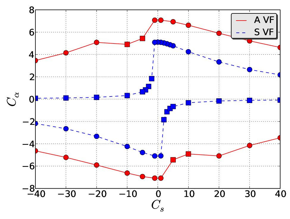
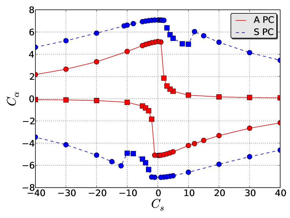
In the rest of this paper we study in more detail the case $C_{S}=-10$ and consider positive values of $C_{\alpha}$. In Fig. 3 we compare the dynamical $\alpha$ quenching model (using a magnetic Reynolds number of $\mbox{\rm Re}_{\rm M}=10^{5}$) with the standard (non-catastrophic) $\alpha$ quenching where $\alpha\propto 1/(1+\overline{\bm{B}}^{2}/B_{\rm eq}^{2})$ with $\overline{\bm{B}}$ being the mean field and $B_{\rm eq}$ the equipartition value. Note that in the former case, the energies cross. Nevertheless, the A solution is stable in both cases – at least for $C_{\alpha}\leq 10$. This is demonstrated in Fig. 4, where we show that after about 40 diffusive times, $\eta_{\rm t}k_{1}t=40$, where $\eta_{\rm t}$ is the turbulent magnetic diffusivity and $k_{1}$ the basic wavenumber, the magnetic energy $E$ decreases and the parity $P$ swaps from $+1$ to $-1$; see Brandenburg et al. (1989) for details on similar studies.

The crossing of the energies in the dynamical quenching model is somewhat surprising. In order to understand this behavior, we need to look at the profiles of the $\alpha$ effect; see Fig. 5. In this model, $\alpha$ is composed of a kinetic part, $\alpha_{\rm K}$, and a magnetic part, $\alpha_{\rm M}$, which has typically the opposite sign, which leads to a reduction of $\alpha=\alpha_{\rm K}+\alpha_{\rm M}$. The quenching can be alleviated by reducing $\alpha_{\rm M}$, for example when the divergence of the magnetic helicity flux of the small-scale field, $\overline{\bm{F}}_{\rm f}$, becomes important.

Naively, we would have expected that the A solution should have a larger energy, because only this solution allows a magnetic helicity flux through the equator; see Fig. 6. This is however not the case, which may have several reasons. Even though the magnetic helicity flux flux small at the equator ($z=0$), there can be significant contributions from within each hemisphere which contributes to alleviating the catastrophic quenching. The details of this will be address in more detail elsewhere.

References

- Brandenburg & Subramanian (2005) Brandenburg, A., & Subramanian, K. 2005, AN, 326, 400
- Brandenburg et al. (1989) Brandenburg, A., Krause, F., Meinel, R., et al. 1989, A&A, 213, 411
- Brandenburg et al. (2009) Brandenburg, A., Candelaresi, S. & Chatterjee, P. 2009, MNRAS 398, 1414
- Manoharan et al. (1996) Manoharan, P. K., van Driel-Gesztelyi, L., Pick, M. & Demoulin, P. 1996, ApJ 468, L73
- Canfield et al. (1999) Canfield, R. C., Hudson, H. S. & McKenzie, D. E. 1999, Geophys. Res. Lett. 26, 627