Electromagnetic response of a highly granular hadronic calorimeter
Abstract
The CALICE collaboration is studying the design of high performance electromagnetic and hadronic calorimeters for future International Linear Collider detectors. For the hadronic calorimeter, one option is a highly granular sampling calorimeter with steel as absorber and scintillator layers as active material. High granularity is obtained by segmenting the scintillator into small tiles individually read out via silicon photo-multipliers (SiPM). A prototype has been built, consisting of thirty-eight sensitive layers, segmented into about eight thousand channels. In 2007 the prototype was exposed to positrons and hadrons using the CERN SPS beam, covering a wide range of beam energies and angles of incidence. The challenge of cell equalization and calibration of such a large number of channels is best validated using electromagnetic processes. The response of the prototype steel-scintillator calorimeter, including linearity and uniformity, to electrons is investigated and described.
keywords
Calorimeter; electromagnetic shower; Silicon Photomultiplier1 Introduction
A new generation of calorimeters that exploit unprecedented high granularity to reach excellent jet energy resolution is one of the main R&D goals towards the future International Linear Collider (ILC) [1]. The particle flow (PFLOW [2, 3, 4]) algorithm favors single particle separability over single particle energy resolution in the attempt to improve the overall jet energy resolution. Typical single hadronic showers in the 10–100 GeV range are best separated in a hadronic calorimeter with cell size of the order of cm2 [4]. In addition, fine longitudinal segmentation is required for PFLOW algorithms to be effective.
The CALICE collaboration [5] is studying several calorimeter designs for experiments at the ILC. With the first generation of prototype detectors new readout technologies have been established for highly granular calorimeters and the stability of these detectors has been demonstrated. Furthermore, a unique set of data has been collected to study hadronic showers at low and medium energies in detail with high resolution longitudinal and transverse sampling.
This paper focuses on the prototype of an analog hadron calorimeter (AHCAL) consisting of 38 layers of highly-segmented scintillator plates sandwiched between 2 cm thick steel plates. Each scintillator tile is an individual calorimeter cell read out by a silicon photo-multiplier (SiPM). Details on the calorimeter structure, calibration and readout electronics are given in Section 2.
Tests using particle beams have been conducted in order to evaluate the performance of the highly granular calorimeters built by CALICE.
In 2007, the whole detector with 38 active layers was commissioned and exposed to muon, positron and pion beams in the energy range 6 GeV to 80 GeV provided by the CERN Super Proton Synchrotron (SPS [11]), on the H6 beam line. In 2008, the AHCAL together with the ECAL and TCMC were moved to the FNAL Meson Test Beam Facility (MTBF [12]) to take data in the 1–6 GeV energy range over the course of two years.
Ongoing data analyses will quantify the energy and spatial resolutions of the prototype for hadrons, and will continue the validation and further development of existing models of hadronic showers, e. g. the various Geant4 [13] physics lists. They will also be important for the experimental validation of the PFLOW approach [14]. The studies in this article focus on the calibration and performance of the device when exposed to electrons and positrons.
In Section 2, the AHCAL is described, and in Section 3 the electromagnetic calibration procedure is discussed. The CERN test beam experiment is described in Section 4. Results on calorimeter response to positrons are given in Section 5, followed by uniformity studies in Section 6. Conclusions are reported in Section 7.
2 Prototype calorimeter


The AHCAL is a sampling calorimeter with alternating 2 cm thick steel plates and highly-segmented scintillator-based active layers. The single calorimeter cell is a scintillator tile read out via a SiPM. The scintillator tiles are 0.5 cm thick and have a size of 3 cm3 cm in the 30 cm30 cm core region and increase to 6 cm6 cm and 12 cm12 cm in the rings surrounding the core. A sketch of one AHCAL module, as well as a picture of an open module showing the arrangement of scintillator tiles, are shown in Figure 1. A wavelength shifting fiber is embedded in the tile, which collects the scintillation light and guides it to the SiPM. The other fiber end is pressed against a 3M reflector foil. The details of one core tile are shown more clearly later in this paper, in the left side of Figure 19. The four sides of each tile are matted by a chemical treatment providing a white surface that serves as a diffuse reflector. The two large faces of the tile are not individually coated, instead a large 3M reflector foil is glued to each side of the metal cassette hosting all tiles providing reflectivity via an air contact. The imperfect reflective coating of the tile edges is responsible for about 2.5 % light cross-talk between neighboring cells of 3 cm edge size.
SiPM devices from the MEPhI/PULSAR group have been used, which have an active area of 1.1 mm 1.1 mm containing 1156 pixels, each 32 m32 m in size. SiPMs are operated with a reverse bias voltage of 50 V, which lies a few volts above the breakdown voltage, resulting in a gain of 106. A poly-silicon quenching resistor on each pixel is used to quench the Geiger discharge. The resistor values vary between 0.5 M and 20 M for the various batches of SiPM produced. Larger resistor values have been favored as they yield a longer pixel recovery time up to 1 s. In this way a pixel cannot be fired multiple times during one scintillator light pulse, though making it easier to monitor the SiPM response curve with LED light. More details on the SiPM working principle and its properties are given in [6, 7].
The active layers are referred to as modules, and the sum of active and passive material adds up to a total depth of 5.3 nuclear interaction lengths (). A more detailed description of the AHCAL prototype structure is given in [8]. The analog SiPM signal is routed to the very-front-end (VFE) electronics where a dedicated ASIC chip [9] is used for multiplexed readout of 18 SiPMs. The integrated components of the ASIC chip allow to select one of sixteen fixed preamplifier gain factors from 1 to 100 mV/pC, and one of sixteen CR–RC2 shapers with peaking times from 40 to 180 ns.
Since the AHCAL was the first detector to employ such a large number of SiPMs, a specialized system for monitoring the long-term stability and performance of the photodetectors was required. In order to monitor the SiPM response function in-situ, a versatile UV LED light distribution system was developed [10]. A calibration and monitoring board (CMB) connected to each module distributes UV light from an LED to each tile via clear fibers. The LEDs are pulsed with 10 ns wide signals steerable in amplitude. By varying the voltage, the LED intensity covers the full dynamic range from zero to saturation (about 70 times the signal of a minimum-ionizing particles). Furthermore, the LED system monitors variations of SiPM gain and signal response, both sensitive to temperature and voltage fluctuations. The LED light itself is monitored with a PIN photo-diode to correct for fluctuations in the LED light intensity.
3 Calibration procedure
One of the aims of the tests discussed here is to establish a reliable and robust calibration chain. This requires measurements with beam particles and with light from the LED monitoring system. The calibration chain is summarized in the following steps:
- •
calibration of the cell response and cell-to-cell equalization;
- •
monitoring of the SiPM gain and corrections for the non-linear response;
- •
calibration to an energy scale (in GeV) with electromagnetic showers.
The cell-by-cell calibration, and with that the equalization of all cell responses, is performed using minimum-ionizing particles (MIPs) provided by a broad muon beam with an approximately Gaussian profile with a width of about 30–40 cm, illuminating all cells in the detector. For each cell, a calibration factor, , is determined from the most probable value of the measured energy spectrum for muons in ADC units, which is extracted with a fit using a Landau function convolved with a Gaussian. This fit accounts for the distribution of energy loss of muons in the scintillator tiles as well as for contributions from photon counting statistics and electronic noise. The combined systematic and statistical uncertainty for these fits was typically on the order of 2%. The muons are generally parallel to the beamline and perpendicular to the detector front face. In this way all cells can be calibrated at the same time, minimizing the impact of temperature induced variations.
The SiPM gain and photo-detection efficiency are temperature dependent. The product of the two determines the SiPM response, which typically decreases by 3.7%/K. A procedure has been developed to correct temperature-induced variations in the calorimeter response using temperature measurements in each module. This procedure and its stability will be described in more detail in [15]. For the analysis presented in this paper, data samples have been selected to cover a temperature range of less than 0.5 K to reduce the impact of such corrections. To account for the included temperature variations, the visible energy of each data set is scaled by -3.7%/K to the average temperature of the muon data used for calibration.
The number of SiPM pixels, , firing for a single cell is related to the ADC value for the cell, , and the corresponding SiPM gain, by . The procedure to obtain the gain of each individual SiPM is discussed in Section 3.1.
The limited number of SiPM pixels leads to a non-linear response for large signals. These effects are corrected for by a function, , depending on the number of fired pixels . This procedure is discussed in detail in Section 3.2.
Finally, a common calibration factor, , scales the visible energy of electrons in each cell in units of MIP to the total deposited energy in units of GeV. This factor is determined to be MIP/GeV, as discussed in Section 5.
Therefore, in summary, the reconstructed energy of electromagnetic showers in the calorimeter is expressed as
| (1) |
where the energy of one single cell with index is . The energy, , given in units of MIP is calculated according to
| (2) |
3.1 SiPM gain and electronics inter-calibration factors
The gain of each individual SiPM is extracted from single photoelectron spectra taken in dedicated runs with low LED light intensity. LED light is necessary as the best determination of the gain requires a single photoelectron spectrum with a Poisson mean of about 1.5 p.e. and the mean obtained from dark noise events is below 0.5 p.e.
The SiPM gain, , is the distance between two consecutive peaks in the single photoelectron spectrum. A typical gain spectrum is shown in Figure 2. A multi-Gaussian fit is performed to the single photoelectron peaks to determine their average relative distance [17]. The mean of each Gaussian function in the multi-Gaussian sum is left as a free parameter. Before fitting, a peak finder routine is used to set each peak mean value to the approximate location of the corresponding photoelectron peak. It has been seen that fixing the distance between peaks to one common parameter reduced significantly the number of converged fits. The width of each Gaussian function is dominated by electronic noise, but for large number of pixels fired the statistical contribution becomes visible, which lead to an increase of the peak width. Accordingly, the width of each peak is left as a free parameter. Finally, the SiPM gain is defined from the fit result as the distance between pedestal (peak zero) and second peak divided by two. An additional consistency check is performed to ensure the distance between pedestal and first peak agrees with the defined gain value at better than 2%. Gaussian fits to peaks higher than the 3rd one are not directly used in determining the gain, but their proper description helps to improve the stablity of the fits and to avoid bias on the peak position. The uncertainty on the gain determination is mainly due to the fit and is about 2 % for fits which pass quality criteria.

SiPM gain measurements were repeated approximately every eight hours during test beam operation. The SiPM gain varies with temperature and the gain measurements can be used to stabilize the calorimeter response over time. The temperature dependence of the SiPM gain is further discussed in [15]. The efficiency of the gain extraction is defined as the number of successful fits in one gain run divided by the number of channels which can be calibrated. About 2 % of all SiPMs are considered inactive because of initially bad soldering or subsequent broken connections to the SiPM leads. Additionally, about 0.11 % of all channels are connected to a broken LED. All these channels are not accounted for in the total of channels that can be calibrated.
The efficiency of the gain extraction with one measurement run is indicative of the quality of the LED monitoring system, namely the small spread of LED light intensity. Figure 3 shows the efficiency of the gain extraction for a series of runs taken in the first three months of data taking at CERN and in the first three months at FNAL. Initial problems during the system commissioning phase led to low efficiency, but after commissioning a gain extraction efficiency of about 95 % per run has been achieved. The gain efficiency was also stable after transportation and throughout the FNAL runs. Combination of several gain runs yields calibration of more than 99 % of all cells. The remaining 1 % of cells are calibrated with the average of the module to which they belong.
The measurement of SiPM gain is performed with a special mode of the readout chip, with a choice of high pre-amplification gain and short peaking time of 50 ns which improves the signal to noise ratio at the single pixel level. In contrast, the muon calibration and the physics data taking are performed with approximately ten times smaller electronic amplification, to optimally fit the available dynamic range, and about 180 ns peaking time to provide sufficient latency for the beam trigger. The inter-calibration factor, , of the chip gain between the calibration mode (CM) and the physics data mode (PM) along with the SiPM gain are used to determine the overall SiPM calibration factor, , used in Eq. 2:
| (3) |


The extraction of the inter-calibration coefficients depends on the linear response of the chip in both modes for an overlapping range of input signals. The input signal is provided by the LED system injecting light into the tiles. The amplitude of the signal is varied within the linear range by varying the LED light intensity. The response in each readout mode is fit with a line, and the ratio between the two slopes is the inter-calibration coefficient for one given readout channel. Ideally, this factor should be a simple constant between the two chip readout modes, but it turns out to depend on the SiPM signal form due to the different shaping times in the two modes. For longer SiPM signals (larger quenching resistor) the inter-calibration is bigger than for shorter SiPM signals (smaller quenching resistor). The inter-calibration factors between the chip readout modes range between 4 and 13.
As with the gain, the inter-calibration extraction efficiency is influenced by the quality of the LED light distribution system. The inter-calibration coefficient extraction efficiencies during the 2007 and the 2008 data taking periods are plotted in Figure 3 (right). After commissioning was completed, all channels with the exception of the 2 % inactive channels and the channels connected to a broken LED, could be inter-calibrated. For the missing inter-calibration values the average of the module to which a SiPM belongs is used instead.
The uncertainty on the inter-calibration coefficient has been estimated from the comparison of several runs and is found to be better than 1 %. Temperature and voltage changes do not affect this coefficient since it is mainly driven by the stability of the components of the readout chip and of the SiPM quenching resistor, all of which are stable in a range of 5–10 degrees.
3.2 SiPM non-linearity
Due to the limited number of pixels and the finite pixel recovery time, the SiPM is an intrinsically non-linear device. The SiPMs used in the AHCAL have a total of 1156 pixels with a recovery time between 25 ns and 1 s, depending on the value of the quenching resistor.
The response function of a SiPM correlates the observed number of pixels fired, , to the effective number of photoelectrons generated, , including cross-talk and after-pulses. The response of a SiPM can be approximated by the function
| (4) |
with the maximum number of fired pixels. This formula is a useful approximation for the case of uniform light distribution over the pixels and short light pulses.
In the above approximation, one can extract a correction function for the SiPM non-linear response as the residual to linearity of the inverted SiPM response function,
| (5) |
In the analysis presented here, we do not directly apply this formula but use tabulated measurements of versus for each SiPM instead. We fit the tabulated measurements with a double exponential function and use this to extract the value of applied in the calibration chain (Eq. 2). The comparison of tabulated AHCAL data with the single and double exponential functions are shown in figure 4 for one example SiPM.

The use of a second exponential in the fitting function does not have a solid physics motivation yet, tough it could be explained thinking of two areas of the SiPM active surface differently illuminated from the WLS fiber. The total number of pixels is divided in two groups, and each of the group is described by an individual exponential function, such that the fitting function is the sum of two exponential functions like that in equation 2. There is no reson for the groups to be exactly two; this method could be extended to more exponentials. For practical reasons though, one needs to limit the number of free parameters. The choice shown in figure 4 turned out to be sufficiently accurate and stable. The correction factor is close to unity for signals of about 30 pixels or 2 MIPs, and increases exponentially up to infinity for signals in saturation.
As illustrated for one SiPM in figure 4, the response curves of each SiPM has been sampled with 20 measurement points on a test bench setup illuminating each SiPM with LED light of variable intensity. For these studies, the SiPMs were not mounted on tiles, but were bare SiPMs. Therefore, all the pixels have been illuminated with light in a homogeneous way. The measurement results for all SiPMs installed in the AHCAL are given in [8]. The maximum number of fired pixels ((bare)) for each SiPM is extracted with a fit to the measured points using Eq.4. The spread (RMS) in the values of between all the curves is about 20 %. SiPMs with 900 have been pre-selected. This ensures not too large variations in the non-linear response function of each device. The 20 measurement points for each SiPMs are stored in a database. A linear interpolation of these points is used to calculate from Eq.5 and linearize the calorimeter response during data reconstruction.

Alternatively, has also been extracted using the AHCAL LED monitoring system from measurements with the with SiPM mounted on a tile ((mounted)). As the saturation point in number of pixels is independent on the linearity of the light, no correction of the LED light intensity with PIN diode has been applied for this study. Figure 5 shows the ratio of (mounted) to (bare). The plot shows that the maximum number of pixels in the in-situ setup is on average 80.5 % of the value determined in the laboratory setup [16] with a wide distribution (RMS=9 %). This factor is interpreted as geometric mismatch between the WLS fiber and the photodetector. The fiber has a 1 mm diameter while the SiPM active surface area is 11 mm2; the geometric ratio between areas is 79 %, in agreement with the measured value. Therefore, only a fraction of the SiPM surface is illuminated and the laboratory curves are re-scaled by the measured value of 80.5 % to correct for this effect before they are used to correct for the SiPM saturation.
The uncertainty of the determination of the saturation point for a single channel is lower than 3 %, if the LED light range properly covers the SiPM saturation region, and if this region is measured well below the ADC saturation. Unfortunately, these conditions are true only for a sub-sample of about 73 % channels. Also judging from the tails in the distribution of Figure 5 some of the fitted results need to be investigated more accurately. For this reason, an average scaling factor is used for all channels. Further studies will address the possibility of using a channel-by-channel factor instead. Furthermore, the measured SiPM response points, from which the correction of non-linear detector response is calculated, are affected by the SiPM gain uncertainty of 2 %, discussed in the following section.
4 The test beam experiment
4.1 The experimental setup at CERN
The data discussed in the following were collected in July 2007 at the CERN SPS test beam facility H6. A sketch of the experimental setup is shown in Figure 6. Apart from the fully equipped AHCAL and a prototype of a tail-catcher and muon tracker (TCMT [18]), the beam installation consists of various trigger and beam monitoring devices. A threshold Čerenkov counter was used to discriminate between electrons and pions. The beam trigger was defined by the coincidence signal of two plastic scintillator counters with cm2 area, referred to as Sc1 and Sc2 in Figure 6. One scintillator trigger (V1), with an area of cm2 and analog read out, tagged multi-particle events. Another scintillator with a cm2 surface and a cm2 hole in the center (V2), was used to reject the beam halo. Three delay wire chambers (DC1, DC2 and DC3) were used to monitor the beam and reconstruct tracks. Events tagged by a scintillator with cm2 area (Mc1), placed behind the TCMT are most likely to be muons.

During most of the tests, a silicon tungsten electromagnetic calorimeter [19] was placed in front of the AHCAL, but this was not the case for the results reported here. The AHCAL was placed on a movable stage, which could shift the detector vertically and horizontally. In addition, the detector can be rotated with respect to the beam direction from an angle of (beam normal to the detector plane) to approximately .
4.2 Monte Carlo simulation
The test beam setup as shown in Figure 6 is simulated with Mokka [20], a Geant4-based [13] Monte Carlo program, followed by a digitization package simulating the response of the detector and electronics. The particle source of the simulation is positioned upstream of the Čerenkov detector. The beam position and spread are chosen to match the beam shapes measured in data by the delay wire chamber, DC3. The beam particles are parallel to the beam axis, according to the measurements in the three delay wire chamber detectors. The material upstream of the AHCAL is simulated. The sub-detectors are simulated with different levels of detail, depending on their impact on the physics analysis: material simulation only for the Čerenkov counter, raw energy depositions stored for the trigger counters, and partial electronics simulation for the tracking detectors. For the AHCAL, the simulation gives the raw energy depositions in a virtual scintillator grid of cm2 tile size. The simulation is followed by a digitization procedure, which takes into account
- •
the realistic detector granularity,
- •
light cross-talk between neighboring tiles,
- •
non-linearity and statistical fluctuations on the pixel scale,
- •
SiPM and readout electronics noise.
The actual geometry of the AHCAL is simulated by summing up the signal yield of 9 (36, 144) virtual cells to obtain those of the actual geometry cells.
Light cross-talk between neighboring cells, due to the imperfect reflective coating of the tile edges, is simulated assuming that from each 3 cm-long tile edge 2.5 % of the scintillator light leaks homogeneously to the neighboring tile. This value is scaled to take into account the fraction of edge shared with the neighbors for cells of different size. The amount of light cross-talk was checked experimentally only for two tiles. The leakage from one tile edge was quantified to be about 2.5 %. No information on the spread of this value between all tiles is given. This value is expected to influence the energy reconstructed and the transverse shower profile. From the comparison of the energy reconstructed in simulation and data, the value of 2.5 % for the light cross-talk on each tile edge is found to be adequate. A light cross-talk of 1.25 % or 3.75 % leads to a difference in the energy scale between data and Monte Carlo larger then 5 %.
To simulate the non-linear behavior of the photodetectors, the energy deposition is translated from GeV to the number of fired SiPM pixels. For this, an intermediate step converts the response simulated in units of GeV to MIP equivalents. The conversion factor is estimated from the simulation of an 80 GeV muon beam in the AHCAL and is found to be 816 keV/MIP, corresponding to the energy lost by a minimum ionizing particle in the scintillator. The amplitude in units of MIPs is then converted into pixels, using the measured light yield for each individual channel. With this scale the measured SiPM response curves from the test bench are used to simulate the SiPM non-linearity. Where not available, the curve of the next neighboring tile is applied.
If is the amplitude in pixels obtained this way and is the saturation level of the individual channel, statistical effects are accounted for by generating a binomial random number with repetitions and a probability of . The result is treated as the number of pixels firing for this specific event, and is translated back to the MIP scale with the channel-specific light yield.
At this stage, the Monte Carlo signal simulated the response of the AHCAL to the energy deposited by particles in an event. However, both the electronic components and the SiPM dark current induce noise. This noise component is assumed to be completely independent of the physics signal in each channel. The noise distribution is non-Gaussian due to the positive SiPM dark noise component. As the frequency of dark noise and the amount of inter-pixels crosstalk varies from SiPM to SiPM, the best way to account for noise is to take it from the data rather than try to simulate it. Noise events for each calorimeter cell are taken from data, are calibrated to the MIP scale according to the reconstruction procedure described in section 3, and are added randomly to the deposited energy of that given cell of a simulated event.
A cell that could not be calibrated in the real detector, either due to an inactive photodetector or to missing calibration values, is also ignored in the simulation. This is about 2 % of the total number of cells in the calorimeter.
5 Calorimeter response to positrons
5.1 Selection of positron events
The analysis presented here is based on positron runs between 10 and 50 GeV. Each energy point has more than 150k recorded beam triggers. All positron runs have been simulated with statistics similar to the corresponding data runs.
Single positron showers are selected for analysis using the beam instrumentation. Although the beam configurations are set to deliver a positron enriched beam, some contamination, mainly from muons, exists. The pion contamination is expected to be negligible, since the tertiary positron beam is produced from a higher-energy mixed beam impinging on a thin (2 ) lead target which does not result in the production of lower-energy tertiary pions. The muon contamination originates from in-flight decay of hadrons upstream of the production target, which results in a muon component that passes the momentum selection.
Cells with a signal above threshold are called hits and MIP is required. To reject empty events that can occur due to random triggers or scattered particles, the number of hits has to be . Furthermore, the energy weighted center-of-gravity in the beam direction (), defined as , has to be mm (about half of the calorimeter depth). This requirement eliminates muons, which deposit their energy equally distributed over the entire calorimeter depth, as opposed to electrons which have a short shower contained in the first half of the calorimeter. It was found that this muon rejection was more efficient than the selection based either on the Čerenkov counter, which does not provide electron-muon separation for 30 GeV and above, or on the muon trigger Mc1 which has an efficiency of about 50%. Particles which interact in the material upstream of the AHCAL are removed by requiring a good track in the delay wire chambers ( 6), and a MIP-like energy deposition in the multiplicity counter (V1). With these selection criteria, 45 % of all recorded events at 10 GeV are accepted. According to Monte Carlo studies 99.9 % of all electron events pass the selection criteria, whereas 99.8 % of all muon events are rejected. The typical fraction of muons in a run is about 5-10 %.
The uncertainty on the mean energy of the beam is reported in [21] to be
| (6) |
The first term is related to hysteresis in the bending magnets while the calibration and the uncertainties on the collimator geometry give the constant term. Since this uncertainty is negligible compared to the detector uncertainties, we assume the beam energy to be fixed. The dispersion of the beam energy can be calculated according to [22] from the settings of the momentum selecting collimators on the beam line and is below 0.24 % for all the runs in this analysis.
5.2 Linearity
The linearity of the calorimeter response for a large range of incident particle energies is a key feature, which allows for an important test of the calibration chain. Electromagnetic showers offer the most rigorous test for non-linearity correction, since the energy deposited per single tile in an electromagnetic shower is larger than that in a hadronic shower for the same particle energy. Figure 7 shows the hit energy spectrum of a 40 GeV positron shower compared to the spectra of 40 GeV and 80 GeV pion showers. The positron shower clearly has more hits with high energy deposition, even when the total particle energy is only half that of the pion.


A set of positron runs with incidence normal to the center of the calorimeter face is analyzed. To minimize the influence of noise, the energy is summed up in a cylinder around the shower axis, where the shower axis is defined by projecting a track formed in the tracking system into the first layer of the AHCAL. This cylinder, sketched in Figure 8 (left), has a radius of 5 Molière radii (, with cm [8]), which ensures a lateral containment of more than 99 % of the shower energy.
The length of the cylinder is chosen to contain the whole shower energy. As suggest by simulations of 50 GeV electron showers, setting L to 20 layers contains the showers. Figure 8 (right) shows the final reconstructed spectra for positron runs in the energy range 10 to 50 GeV. The positrons are normally incident on the calorimeter front face, with a distribution centered in the same calorimeter cell for each run. The distribution is fit with a Gaussian function in the range . The position of the peak is taken as the mean energy response, , measured in units of MIP. The reconstructed energy of a 10 GeV positron shower is compared to the digitized energy from a Monte Carlo simulation in Figure 9. The agreement between data and simulation is satisfactory.

The statistical uncertainties on the mean energy deposition are negligible. The main source of systematic uncertainties is 2 % from MIP scale calibration. The uncertainty of 2 % on the SiPM gain determination, resulting from the fit stability and the uncertainty on the determination of the SiPM saturation level both affect the correction of the SiPM non-linear response. For the saturation level a common re-scaling factor is applied to all SiPM curves determined in the laboratory setup. The rescaling is needed to account for the partial illumination of the SiPMs from the WLS fiber as discussed in Section 3.2. As shown in Figure 5, the ratio between the in-situ measured SiPM saturation level and the test-bench determined value has a wide distribution. Since a common factor of 80.5 % is used to rescale all SiPM response curves, an uncertainty of 11.3 % on this value is assumed, which represents the spread of all measured values as taken from Figure 5. To account for this uncertainty in an uncorrelated way for all SiPMs, 100 experiments have been performed assigning different rescaling coefficients for each channel, generated randomly with a Gaussian distribution centered at 0.80 and with a sigma of 0.09. For each experiment the energy in the calorimeter is reconstructed, using the set of curves rescaled by these randomly generated coefficients to correct the non-linear SiPM response. Finally, the one standard deviation spread of the 100 reconstructed energies from these simulated experiments is taken as the systematic uncertainty for the reconstructed energy. All of the above listed systematic uncertainties are uncorrelated and thus added in quadrature. The total systematic uncertainty ranges from (2 %) at 10 GeV to 1.7 GeV (3.4 %) at 50 GeV.
The reconstructed energy in GeV is obtained as , where is the electromagnetic energy scale factor (MIP-to-GeV). The scale factor is determined with a linear fit from zero to 50 GeV to the distribution versus . The resulting values for data and Monte Carlo are MIP/GeV and MIP/GeV, respectively. Within the uncertainties, the scale factors are in good agreement.
| Data | MC | ||||||
|---|---|---|---|---|---|---|---|
| [%] | [%] | [%] | [GeV] | [GeV] | |||
| 10 | 9.9 | 2.0 | 0.3 | 0.4 | 0.2 | 9.9 | 0.2 |
| 15 | 15.0 | 2.0 | 0.5 | 0.8 | 0.3 | 15.0 | 0.3 |
| 20 | 20.1 | 2.0 | 0.7 | 1.2 | 0.5 | 20.2 | 0.5 |
| 30 | 29.9 | 2.0 | 1.1 | 1.8 | 0.9 | 30.4 | 0.9 |
| 40 | 39.3 | 2.0 | 1.2 | 2.3 | 1.3 | 40.8 | 1.3 |
| 50 | 48.3 | 2.0 | 1.4 | 2.6 | 1.7 | 51.0 | 1.8 |

The linearity of the AHCAL response to positrons is shown in Figure 10. A comparison of the data before and after correction for the SiPM non-linear response indicates the magnitude of this correction, which does not exceed 10 % even at 50 GeV positron energy. The values shown in Figure 10 are reported in Table 1.
The residuals for data and Monte Carlo are presented in Figure 11. Here, the green band indicates the quadratic sum of the energy dependent systematic uncertainties. In Table 1 the contribution to the uncertainty from the SiPM gain variation, , and from the saturation point determination, are listed. The uncertainty on the MIP scale, , cancels in the ratio since the same calibration constants are used in data and Monte Carlo. In Figure 11 (left), the residuals from the linear function suggests a non-zero offset at zero energy. This negative offset is the combined effect of the 0.5 MIP threshold (loss of energy) and the detector noise (addition of energy). Instead of the more conventional linear function with , the function can be used to fit the data in the range 10–50 GeV. A value of MeV is found for the Monte Carlo offset. Once this offset is removed the Monte Carlo linearity is better than 0.5 % over the whole range, as shown in the right plot of Figure 11.


The deviation from linearity (Fig. 11 left) in data is less than 1 % in the range 10 to 30 GeV and the maximum deviation is about 3 % at 50 GeV. The remaining non-linearity at high energies hints at problems with the rescaling of the saturation curves, as described in Section 3.2. This behavior is not sufficiently reproduced in the Monte Carlo digitization, where the same curve is used to simulate saturation as is used to correct for it.
The impact of the saturation correction is better seen in Figure 12 where the energy per hit is shown with and without the correction factor applied, for 30 GeV electromagnetic showers. Whereas the correction is negligible for low signal amplitudes, it becomes significant at larger amplitudes, resulting in a strong correction for the tail of the distribution. The maximum energy deposited in one cell for a 30 GeV electromagnetic shower is 230 MIPs corresponding to about 3450 pixels (assuming a light yield, LY = 15 pixel/MIP). For this amplitude the correction factor is . The remaining miss-match between data and Monte Carlo around 100-200 MIPs is an effect of the non-perfect correction of the non-linear SiPM response. This imperfect correction affects only a small fraction of the total energy; the hits above 50 MIPs contribute only 0.5 % (4 %) of the total energy at 10 GeV (40 GeV).


5.3 Electromagnetic energy resolution
Energy resolution is a principal figure of merit in calorimetry and is estimated as the width divided by the mean of a Gaussian fit to the energy sum within of the mean of an initial fit over the full range. The resolution achieved with the AHCAL is plotted as a function of the beam energy in Figure 13. The values shown in this figure are reported in Table 2. Fitting the AHCAL energy resolution in a range of , with
| (7) |
results in a stochastic term of , whereas the constant term is . The noise term of MeV is extracted from the spread (RMS) of the random trigger event distribution and kept constant during the fitting procedure. The energy resolution agrees well with that of an earlier prototype (Minical) with 108 channels and of the same sampling [24], that was tested in the energy range between 1 and 6 GeV and reached a resolution with a stochastic term and a constant term .

The energy resolution of the simulation is found to have a stochastic term of , a constant term of and again a fixed noise term of MeV. Within the fit uncertainty, the stochastic terms of data and simulation are in good agreement. The noise term is fixed to the same value as for data since the noise in the simulation is artificially added from random trigger data events. The constant term , representing calibration uncertainties and non-linearities, is consistent with zero in the simulation as expected, since the same curves are both in the simulation of the non-linear SiPM response and in its correction.
| Data | MC | |||
|---|---|---|---|---|
| [GeV] | [%] | Uncertainty [%] | [%] | Uncertainty [%] |
| 10 | 7.11 | 0.47 | 6.90 | 0.49 |
| 15 | 5.83 | 0.36 | 5.45 | 0.38 |
| 20 | 4.95 | 0.32 | 4.90 | 0.34 |
| 30 | 3.97 | 0.29 | 4.00 | 0.31 |
| 40 | 3.54 | 0.26 | 3.51 | 0.27 |
| 50 | 3.41 | 0.25 | 3.07 | 0.26 |
5.4 Shower profiles
The longitudinal profile of a shower induced by a particle with incident energy in GeV traversing a matter depth can be described as [23]
| (8) |
where the parameter is an overall normalization, and the parameters and are energy and material-dependent. The first term represents the fast shower rise, in which particle multiplication is ongoing, and the second term parametrizes the exponential shower decay. Given this parametrization with in units of radiation lengths, the particle multiplication and the energy deposition reach their maximum after
| (9) |
radiation lengths from the beginning of the cascade of a particle with energy . The critical energy, is a property of the calorimeter material and does not depend of the energy of the particle. The position is called the shower maximum.


The mean longitudinal profile of a 10 GeV positron shower is shown in the left plot of Figure 14. Due to the high longitudinal segmentation of the AHCAL, the shower rise, maximum and decay are clearly visible. Data and simulation are in qualitatively good agreement. To quantify this agreement, the profiles at each recorded beam energy are fitted with Eq. 8 and the maximum shower depth calculated as . The development of the shower maximum as a function of the beam energy is shown in the right plot of Figure 14. The error bars show the uncertainty from the fits. The extracted shower maxima of both data and simulation are in good agreement with the theoretical behavior for a pure Fe calorimeter with a critical energy, from [23], of MeV, given in Eq. 9.
The transverse shower profile of a 15 GeV positron shower is shown in Figure 15 together with a simulation. The radius, , is calculated with respect to the track of the incoming particle extrapolated from the tracking system to the AHCAL front face. Therefore, the radius is defined as , where () are the coordinates of the calorimeter cell with signal above threshold. The energy deposited in a calorimeter cell is normally assigned to the center of the cell. For the radial profile studies it is redistributed uniformly in bins of 1 mm2 before being assigned to one annular bin of inner radius . In this way the energy deposited in one calorimeter cell can be shared between two adjacent annular bins. Proper normalization accounts for the fraction of the calorimeter cell area covered by each annular bin.


The data indicate a broader shower than expected from simulation. The calculated mean shower radius () for 15 GeV showers in data is about 9 % larger than the simulated one.
The energy dependence of is shown on the right plot of Figure 16 (left). The difference is almost energy independent. For completeness also the comparison of the RMS () of the shower radius distribution is shown in Figure 16 (right). An energy dependent disagreement of data and Monte Carlo is observed for this variable which increases to a maximum of 7 % for 50 GeV. Several studies have been performed to find the cause of this effect including noisy and inactive cells, different beam shape, influence of the light cross-talk between tiles, misalignment between calorimeter and tracking system and of calorimeter layers. The broader shower in data is still not understood and further studies of asymmetric light collection on the tile, the influence of varying dead space between tiles due to varying thickness of reflector coating, etc., will follow to investigate the discrepancy. For the purpose of the validation of the calibration procedure the current level of agreement is acceptable, though this mismatch will have to be taken into account when comparing hadronic shower shapes. Furthermore, hadronic showers have a much smaller energy density than electromagnetic showers; therefore, any local effects, (i.e. the impact of dead areas or misalignment between layers), are strongly amplified in electromagnetic showers, while the influence is expected to be much less pronounced in hadronic showers.
6 Uniformity studies
6.1 Uniformity of the calorimeter response
The uniformity of the AHCAL response is explored by shifting the AHCAL to different positions with respect to the beam axis, at normal angle of incidence. This procedure is visualized in the left part of Figure 17. Each square in the sketch represents one scintillating tile of cm2 and beam events with a track pointing to a 11 cm2 region centered on each tile in turn were selected. The uniformity of the calorimeter response at the 15 different positions has been tested. For this study 10 GeV positron runs are analyzed, where the movable stage was used to displace the calorimeter in the - position with respect to the beam-line (-axis).
As shown in the right plot of Figure 17, when excluding position 10, the uniformity of the calorimeter response is better than 2.1 %. The 10 % deviation between reconstructed and beam energy at position 10 is due to an inactive cell at the shower maximum, which is not corrected in the calibration.


6.2 Angular dependence of the calorimeter response
The movable stage carrying the AHCAL was used to collect positron data at incident angles of , , and . The rotation and staggering of the AHCAL are sketched in the left plot of Figure 18, where the beam is entering from the top. In the rotated configuration, the modules were staggered to ensure the highly granular core of 33 cm2 was aligned with, and hence sampled, the shower core.

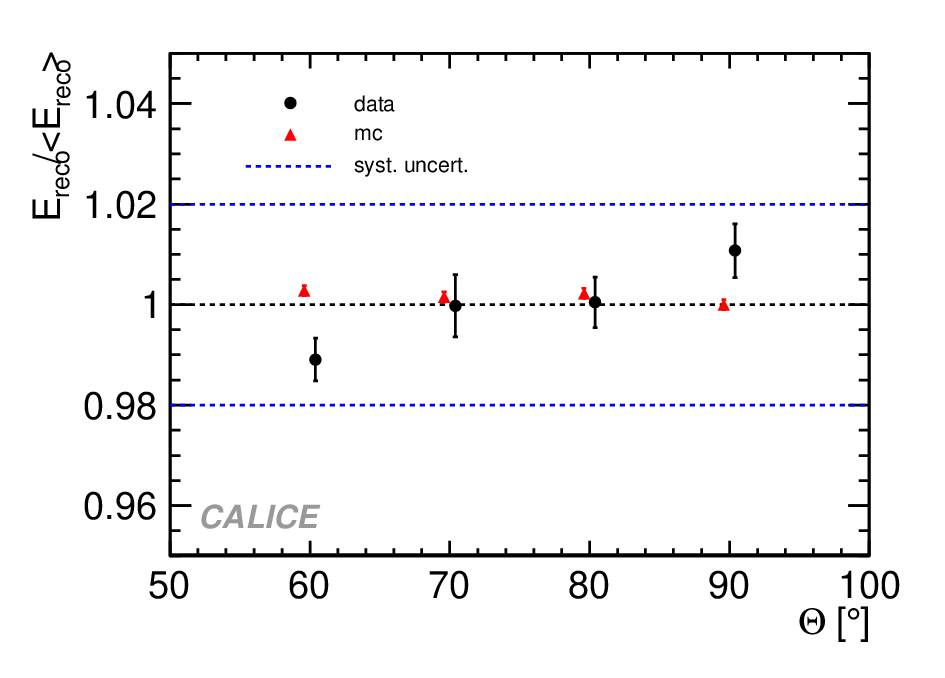
For each angle of incidence several 10 GeV positron runs with different impact points on the calorimeter front surface were taken. The average of all the runs is used to define at one given , while is the mean reconstructed energy at any angle of incidence. The normalized reconstructed energy is plotted in Figure 18 as a function of . The spread (RMS) between the various analyzed runs per inclination angle is used as the systematic uncertainty. This spread is smaller than the calibration systematic uncertainty in the calorimeter, shown in the plot as an error band around the ratio of one. Showers at various inclination angles only partially share the same calorimeter cells, therefore the full systematic uncertainty from calibration is an overestimate of the real error, but the spread between measurements performed at one inclination angle is an underestimate. Taking this into account, the increase in the reconstructed energy of data between and is not significant. A more precise analysis would require more data at different angles which are not available at present.
6.3 Influence of cell structure
The scintillating tiles used in the AHCAL have a WLS fiber embedded in a groove, a SiPM inserted into a small groove on one end of this fiber, and a mirror in a groove on the other end. This structure is visible in the picture of a cm2 tile in Figure 19, where the SiPM is located in the lower left-corner, the mirror is placed in the diagonal corner, and the WLS fiber is embedded in a quarter circle.
Since electromagnetic showers have a short transverse extension, the impact of the cell structure slightly reduces the energy resolution of the calorimeter. To study this effect, we take advantage of the delay wire chambers that were present in the beam line. They are used to reconstruct the track of the incoming particle. This track is then extrapolated to the front face of the AHCAL. The shower energy (energy summed over the entire calorimeter) for 10 GeV positrons with this impact position, normalized to the shower energy averaged over all impact positions, is plotted in Figure 19.


As shown in the figure, the measured energy drops slightly over the area of the WLS fiber. A particle with a trajectory intersecting the SiPM (in the lower left corner of the plot) or the reflecting mirror at the end of the WLS fiber (in the upper right corner of the plot) shows a significant loss of response with respect to the tile average by about 8 % and 4 % respectivley. At the position of the WLS fiber the tile response is about 2 % lower than average. The drop at the other two corners of the tile in this study reflects the energy loss associated with the SiPMs located in the neighboring tiles as the observable used is the energy summed over the entire calorimeter. Measurements of single tile uniformity using a collimated source have been performed and are reported in [25, 26]. These measurements confirm a lower response of electromagnetic showers hitting the SiPMs or the reflecting mirrors. Though this large degradation (8 % at the locations of the SiPMs) is quite unrealistic in a collider detector, where the particles are always traversing the calorimeter under an angle. In this case the tile response non-uniformity averages out with no influence on the energy resolution. Furthermore, electromagnetic showers have a short lateral extension. For pion showers, which are much wider, the effect has not been observed in data. The effects of gaps between the calorimeter tiles, as well as the non-uniform response of the tiles, in view of the impact on the energy resolution, have been studied using Monte Carlo events. The results are reported in [27] and show that these type of effects do not have a significant influence on the measurement of hadron showers.
7 Conclusions
The response of the CALICE analog hadron calorimeter to positrons was measured for energies between 10 and 50 GeV, using data recorded at CERN in summer 2007. The calorimeter response is linear to better than 3 %. A better SiPM saturation correction would improve the linearity, and for future developments a larger dynamic range is desirable. This study is ongoing, but the effect on pion energy reconstruction will be negligible due to the much smaller energy per hit in a hadronic shower compared to an electromagnetic shower. The energy resolution for positrons is found to have a stochastic term of %, and a constant term of about 1 %. Good agreement between data and simulation validates the simulation of the various detector characteristics. For comparison, Ref. [28] reports for the ATLAS tile calorimeter an energy resolution of 28 % stochastic and 2.8 % constant term for electrons at 20 deg from normal incidence. This is also and hadron sampling calorimeter alternating steel and scintillator tiles, but with a much coarser granularity than the AHCAL and a different a readout via standard photomultiplier tubes. The same readout technology as in the AHCAL is also implemented in a scintillator-Tungsten electromagnetic calorimeter, ScECAL build within the CALICE collaboration [29]. For this calorimeter the energy resolution to electrons is of % stochastic and % constant term. This analysis provided confidence that the detector performance and simulation are sufficiently understood to pursue the investigation of hadronic showers.
Systematic studies are performed to investigate the quality of the calibration in as many calorimeter cells as possible. The uniformity of the calorimeter response to electromagnetic showers is studied with beams at different impact points and different incident angles. The results are consistent with no angular and spatial dependence within the quoted systematic uncertainty on the calibration procedure.
The high segmentation of the AHCAL is well-suited for studying the longitudinal shower development with high accuracy and for determining the shower maximum. The point of maximum energy deposition along the shower propagation axis is located between 5.5 and 7 for the range of particle energies used, consistent with simulation and theoretical prediction.
The transverse shower spread is more difficult to measure because it is strongly affected by uncertainties in the beam profile, in the variation of light cross-talk between tiles, and in the misalignment of calorimeter layers. Currently, the data indicate a broader shower than expected from simulation. However, the level of agreement is acceptable for the validation of the calibration procedure if one considers that the effect on hadronic showers will be less important due to the lower energy density of hadronic showers.
Acknowledgements.
We would like to thank the technicians and the engineers who contributed to the design and construction of the prototypes. We also gratefully acknowledge the DESY and CERN managements for their support and hospitality, and their accelerator staff for the reliable and efficient beam operation. This work was supported by the Bundesministerium für Bildung und Forschung (BMBF), grant no. 05HS6VH1, Germany; by the DFG cluster of excellence ‘Origin and Structure of the Universe’ of Germany ; by the Helmholtz-Nachwuchsgruppen grant VH-NG-206; by the Alexander von Humboldt Foundation (Research Award IV, RUS1066839 GSA); by joint Helmholtz Foundation and RFBR grant HRJRG-002, SC Rosatom; by Russian Grants SS-3270.2010.2 and RFBR08-02-12100-OFI and by Russian Ministry for Education and Science; by MICINN and CPAN, Spain; by CRI(MST) of MOST/KOSEF in Korea; by the US Department of Energy and the US National Science Foundation; by the Ministry of Education, Youth and Sports of the Czech Republic under the projects AV0 Z3407391, AV0 Z10100502, LC527 and LA09042 and by the Grant Agency of the Czech Republic under the project 202/05/0653; and by the Science and Technology Facilities Council, UK.References
- [1] N. Phinney et al., Reference Design Report Volume 3: Accelerator, available at http://lcdev.kek.jp/RDR/
- [2] J.-C. Brient, Improving the jet reconstruction with the particle flow method: An introduction, in the Proceedings of the 11th International Conference on Calorimetry in High-Energy Physics (CALOR 2004), Perugia, Italy, March 2004.
- [3] V.L. Morgunov, Calorimetry Design with Energy-Flow Concept, in 10th International Conference on Calorimetry in High Energy Physics (CALOR 2002), Pasadena, CA, U.S.A., March 2002.
- [4] M. A. Thomson, Particle Flow Calorimetry and the PandoraPFA Algorithm, arXiv:0907.3577 [physics.ins-det], Nucl. Instrum. Meth. A 611 (2009) 25-40.
- [5] The CALICE collaboration, see https://twiki.cern.ch/twiki/bin/view/CALICE/WebHome
- [6] The CALICE/SiPM collaboration, B. Dolgoshein et al., Status report on silicon photomultiplier development and its applications, Nucl. Instrum. Meth. A 563 (2006) 368.
- [7] P. Buzhan et al., Silicon photomultiplier and its possible applications, Nucl. Instrum. Meth. A 504 (2003) 48.
- [8] The CALICE collaboration, C. Adloff et al., Construction and commissioning of the CALICE Analog Hadron Calorimeter Prototype, arXiv:1003.2662 [physics.ins-det], JINST 5 (2010) P05004.
- [9] S. Manen et al., Dedicated front-end electronics for the next generation of linear collider electromagnetic calorimeter, presented at the 10th Workshop On Electronics For LHC and Future Experiments, Boston, USA, September 2004, arXiv:physics/0501063.
- [10] N. Wattimena, Commissioning of an LED Calibration & Monitoring System for the Prototype of a Hadronic Calorimeter, DESY-THESIS-2006-039 (2006). And Calorimetry at the International Linear Colider. From Simulation to Reality, DESY-THESIS-2010-006 (2010).
- [11] Description of the CERN H6 testbeam area available at http://sl.web.cern.ch/sl/eagroup/beams.html#h6.
- [12] Description of the FNAL MTBF testbeam area available at http://www-ppd.fnal.gov/MTBF-w/.
- [13] The Geant4 collaboration, S. Agostinelli et al., Geant4 - A Simulation Toolkit, Nucl. Instrum. Meth. A 506 (2003) 250-303.
- [14] O. Markin, Pandora PFA tests using overlaid charged pion test beam data, in 14th International Conference on Calorimetry in High Energy Physics (CALOR 2010), Beijing, China, May 2010.
- [15] The CALICE collaboration, C. Adloff et al., Muon response of a highly granular Hadronic Calorimeter, in preparation.
- [16] N. Feege, Silicon Photomultipliers: Properties and and Application in a Highly Granular Calorimeter, DESY-THESIS-2008-050 (2008).
- [17] B. Lutz, Commissioning of the Readout Electronics for the Prototypes of a Hadronic Calorimeter and a Tailcatcher and Muon Tracker, DESY-THESIS-2006-038 (2006). And Hadron showers in a highly granular calorimeter, DESY-THESIS-2010-048 (2010).
- [18] D. Chakraborty, The Tail-Catcher/Muon Tracker for the CALICE Test Beam, in the Proceedings of 2005 International Linear Collider Workshop (LCWS 2005), Standford, California, March 2005.
- [19] M. Anduze et al., Design and Commissioning of the Physics Prototype of a Si-W Electromagnetic Calorimeter for the International Linear Collider, JINST 3 (2008) P08001.
- [20] Mokka Geant4 Application for Linear Collider Detectors, see http://polzope.in2p3.fr:8081/MOKKA.
- [21] The CALICE collaboration, C. Adloff et al., Response of the CALICE Si-W electromagnetic calorimeter physics prototype to electrons, Nucl. Instrum. Meth. A 608 (2009) 372.
- [22] Short Introduction to the use of the H6 beam, see http://sba.web.cern.ch/sba/BeamsAndAreas/h6/H6manual.pdf
- [23] C. Leroy and P. Rancoita, Physics of cascading shower generation and propagation in matter: Principles of high-energy, ultrahigh-energy and compensating calorimetry, Rept. Prog. Phys. 63 (2000) 505.
- [24] V. Andreev et al., A high granularity scintillator hadronic-calorimeter with SiPM readout for a linear collider detector, Nucl. Instrum. Meth. A 540 (2005) 368.
- [25] M.Danilov International Linear Collider Workshop 2008, Chicago, November 16-20, 2008 (http://www.linearcollider.org/lcws08/).
- [26] F. Simon and C. Soldner, Uniformity Studies of Scintillator Tiles directly coupled to SiPMs for Imaging Calorimetry, Nucl. Instrum. Meth. A 610 (2010) 196. 10.1016/j.nima.2010.03.142.
- [27] A.Lucaci-Timoce, F. Sefkow, Monte Carlo Studies of the CALICE AHCAL Tiles Gaps and Non-uniformities in the Proceedings of 2005 International Linear Collider Workshop (LCWS 2010), arXiv:1006.3662 [physics.ins-det].
- [28] P. Adragna et al., Testbeam Studies of Production Modules of the ATLAS Tile Calorimeter, Nucl. Instrum. Meth. A 606 (2009) 362. 10.1016/j.nima.2009.04.009.
- [29] A. Kahn, Scintillator-Based Electromagnetic Calorimeter Prototype and Beam Test Results at FNAL, in the Proceedings of International Linear Collider Workshop 2010 (LCWS10 and ILC10), March 26-30, 2010 China arXiv:1007.2553 [physics.ins-det].