On the color suppressed contribution to
Abstract
The decay modes of the type are dynamically different. For the case there is a substantial factorized contribution which dominates. In contrast, the decay mode has a small factorized contribution, being proportional to a small Wilson coefficient combination. However, for the decay mode there is a sizeable nonfactorizable (color suppressed) contribution due to soft (long distance) interactions, which dominate the amplitude.
We estimate the branching ratio for the mode in the heavy quark limit for the - quark. In order to estimate color suppressed contributions we treat the energetic light () quark within a variant of Large Energy Effective Theory combined with a recent extension of chiral quark models in terms of model- dependent gluon condensates.
We find that our calculated color suppressed amplitude is suppressed by a factor of order with respect to the factorizable amplitude, as it should according to QCD-factorization. Further, for reasonable values of the constituent quark mass and the gluon condensate, the calculated nonfactorizable amplitude for can easily accomodate the experimental value. Unfortunately, the color suppressed amplitude is very sensitive to the values of these model dependent parameters. Therefore fine-tuning is necessary in order to obtain an amplitude compatible with the experimental result for . A possible link to the triangle anomaly is discussed.
Keywords:
-decays, factorization, gluon condensate.
PACS: 13.20.Hw , 12.39.St , 12.39.Fe , 12.39.Hg.
I Introduction
Due to numerous experimental results coming from BaBar and Belle, there is presently great interest in decays of -mesons. LHC will also provide us with more data for such processes. -decays of the type and , where the energy release is big compared to the light meson masses (heavy to light transitions), has been treated within QCD factorization [1] and Soft Collinear Effective Theory (SCET) [2]. In the high energy limit, the amplitudes for such decay modes factorize into products of two matrix elements of weak currents, and some nonfactorizable corrections of order can be calculated perturbatively. However, there are additional contributions of order which cannot be reliably calculated within perturbative theory [1]. The so called pQCD-model and QCD sum rules have also been used for -meson decays [3, 4].
For decay modes which are of the heavy to heavy type, involving - and -quarks, the decay amplitudes have been described within Heavy Quark Effective Field Theory (HQEFT) [5]. Some transitions of heavy to heavy type in the heavy quark limits like mixing [6] has been studied within Heavy Light Chiral Perturbation Theory (HLPT) [7]. Furthermore, other transitions which are formally heavy to heavy in the heavy quark limits and , like the Isgur-Wise function [8] for , have been studied within HLPT [7]. The cases [9] and [10, 11] have also been studied within such a framework, even if the energy release in these processes is above the chiral symmetry breaking scale. Still this framework give amplitudes of the right order of magnitude. The calculation of such transitions have in addition been supplemented with calculations within a Heavy Light Chiral Quark Model (HLQM) to determine quantities which are not determined within HLPT itself [12, 9, 11].
As pointed out in a series of papers [12, 9, 11, 13], there are processes which have factorized amplitudes multiplied by a very small Wilson coefficient combination, such that nonfactorized amplitudes are expected to dominate. Examples are [9] , [12] and . The latter process was considered recently [13, 14]. In that case a heavy -quark decaying to a light, but energetic quark was involved. Then the light energetic quark might be described by an effective theory. The first version of such a framework was Large Energy Effective Theory (LEET) [15, 16]. The HQEFT covers processes where the heavy quarks carry the main part of the momentum in each hadron. To describe processes where energetic light quarks emerge from decays of heavy -quarks, LEET was introduced [15] and used to study the current for [16].
The idea was that LEET should do for energetic light quarks what HQEFT did for heavy quarks. In HQEFT one splits off the heavy motion from the full heavy quark field, thus obtaining a reduced field depending on the velocity of the heavy quark. Similarly, in LEET one splits off the large energy from the full field of the energetic light quark, thus obtaining an effective description for a reduced light quark which depends on a light-like four vector. It was later shown that LEET in its initial formulation was incomplete and did not fully reproduce QCD physics [17]. Then LEET was further developed to be fully consistent with QCD and became the Soft Collinear Effective Theory (SCET) [2].
In the present paper we consider decay modes of the type . The decay mode has a substantial factorized amplitude, given by the current matrix element for transition times the matrix element of the weak current for the outgoing , which is proportional to the pion decay constant . The relevant Wilson coefficient is also the maximum possible, namely of order one times the relevant Cabibbo-Kobayashi-Maskawa (CKM) quark mixing factors and the Fermi coupling constant. This is in contrast to the process which is color suppressed. As said above, decays of the type have been extensively studied within QCD-factorization, SCET, and QCD sum rule methods [18]. In spite of tremendous efforts it has not been possible to obtain an amplitude compatible with the experimental result . The purpose of this paper is study this decay mode within an alternative model dependent framework.
First we point out that the factorized contribution to the decay mode , which is given by the transition amplitude times the decay constant of the meson, is almost zero because it is proportional to a very small Wilson coefficient combination. For the dominant nonfactorizable (color suppressed) amplitude for we will, as mentioned above, use a model named Large Energy Chiral Quark Model (LEQM) recently constructed and used to handle the process [14, 13]. Here a variant of LEET was combined with ideas from previous chiral quark model (QM) calculations similarly to what has been done for other nonleptonic decays [20, 6, 12, 11, 19].
A priori it might look strange to use the framework of chiral quark models when the energy release is big compared to the chiral symmetry breaking scale . The point is that the motion of the heavy quark or energetic light quark can be split off, and the various versions of heavy-light or large energy chiral quark models and a corresponding chiral perturbation theory () can be used to describe the redundant strong interactions corresponding to momenta of order 1 GeV and below.
It might be argued that we should have used the full SCET theory as the basis our new model. However, the purpose of our paper is to estimate, in analogy with previous papers [6, 21, 12, 11, 20, 22, 19, 23], the effects of soft gluon emission in terms of gluon condensates, where transverse quark momenta and collinear gluons will not play an essential role. In any case this construction [13] will be a model. Therefore it suffices for our purpose to use the more simple formulation of LEET. We will combine LEET with chiral quark models (QM) [24, 25, 26, 27, 21], containing only soft gluons making condensates. In LEQM [13] an energetic quark is bound to a soft quark with an a priori unknown coupling, as proposed in [21]. The unknown coupling is determined by calculating the known current matrix element within the model [13]. This fixes the unknown coupling because the matrix element of this current is known [16]. Then, in the next step, we use this coupling to calculate the nonfactorized (color suppressed) amplitude contribution to in terms of the lowest dimension gluon condensate, as have been done for other nonleptonic decays [20, 6, 12, 11, 19]. After the quarks have been integrated out, we obtain an effective theory containing soft light mesons as in HLPT, but also fields describing energetic light mesons. A similar idea with a combination of SCET with HLPT is considered in [28]. The LEQM was constructed in analogy with the previous Heavy Light Chiral Quark Model (HLQM)[20] and may be considered to be an extension of that model.
One might think that to be completely consistent, we should also have calculated the Wilson coefficients within a relevant large energy framework. For this purpose the use of LEET would be dubious because it is an incomplete theory as mentioned above. However, as we will see below, the main uncertainty in our final amplitude will be due to uncertainty in our model dependent gluon condensate due to emission of soft gluons. Therefore the Wilson coefficients calculated within full QCD as in [29] will be appropriate for our purpose.
In the next section (II) we present the weak four quark Lagrangian and its factorized and nonfactorizable matrix elements. In section III we present our version of LEET, and in section IV we present the new model LEQM to include energetic light quarks and mesons. In section V we calculate the nonfactorizable matrix elements due to soft gluons expressed through the (model dependent) quark condensate. In section VI we give the results and conclusion.
II The effective Lagrangian at quark level
We will study decays of generated by the weak quark process . We restrict ourselves to processes where the -quark decays. This means the quark level processes . Processes where the anti- -quark decays proceed analogously. The effective weak Lagrangian at quark level is [29] (neglecting penguin operators)
| (1) |
where the subscript denotes the left-handed fields: , where is the left-handed projector in Dirac-space. The local operator products are defined as
| (2) |
In these operators summation over color is implied. In Eq. (1), and are Wilson coefficients. At tree level and . At one loop level, a contribution to is also generated, and is slightly increased. These effects are handled in terms of the Renormalization Group Equations (RGE)[29], and the coefficients can be calculated at for instance or = 1 GeV. Using the color matrix identity
and Fierz rearrangement, the amplitudes for the processes may be written as
| (3) | |||||
and for
| (4) | |||||
Here the terms proportional to and with color matrices inside the matrix elements are the genuinely nonfactorizable contributions.
Since is of order one and of order [12, 13] , we refer to the coefficients
| (5) |
as favorable () and nonfavorable () coefficients, respectively. Thus, the decay mode has a sizeable factorized amplitude proportional to . In contrast, the decay mode has a factorized amplitude proportional to the nonfavorable coefficient which is close to zero. In this case we expect the nonfactorizable term (involving colour matrices) proportional to to be dominant, i.e. the last line of eq. (4) dominates. A substantial part of this paper is dedicated to the calculation of this nonfactorizable contribution to the decay amplitude.
Thus the main task of this paper will be to calculate the matrix element of the operator consisting of the product of two colored currents occurring in the last line of eq. (4):
| (6) |
for the color suppressed process . This matrix element will be estimated in section V where we use the LEQM to estimate nonfactorizable amplitudes in terms of emission of soft gluons making gluon condensates.
III An energetic light quark effective description (LEET)
An energetic light quark might, similarly to a heavy quark, carry practically all the energy of the meson it is a part of. The difference is that now the mass of the energetic quark is close to zero compared to the heavy quark mass and , which are assumed to be of the same order of magnitude. We assume that the energetic light quark is emerging from the decay of a heavy quark with momentum . The heavy quark is described by the HQEFT Lagrangian for the reduced quark field [5]:
| (7) |
where is the reduced heavy quark field (often named in the literature), its four velocity and the mass of the heavy quark.
The momentum of the light energetic light quark can be written
| (8) |
where , which is of order , is the energy of the energetic light quark, is the light quark mass. Further, is the light-like four vector wich might be chosen to have the space part along the z-axis, , in the frame of the heavy quark where . Then and . Inserting this in the regular quark propagator, In the limit where the approximations in (8) are valid, we obtain the propagator
| (9) |
This propagator is the starting point for the Large Effective Theory (LEET) constructed in Ref. [16].
Unfortunately, the combination of LEET with QM will lead to infrared divergent loop integrals for (see section IV). Therefore, the formalism was modified [14, 13] and instead of , we use , with where , such that . An expansion in will then within our model be equivalent to an expansion in .
In the following we describe the modified LEET [16] where we keep with . We call this construction LEET [13] and define the almost light -like vectors
| (10) |
where . This means that
| (11) |
In the following we use the projection operators given by
| (12) |
where . One factors out the main energy dependence, just as was analogously done in HQEFT, and define the projected reduced quark fields[16]
| (13) |
As in [16], the field was eliminated and one obtained for the effective Lagrangian [13]:
| (14) |
which (for ) is the first part of the SCET Lagrangian. The operator is given in [13]. Equation (14) yields the LEET quark propagator
| (15) |
which reduces to (9) in the limit . In addition, for a light energetic quark, the propagator within SCET [2] will for small transverse quark momenta coincide with Eq. (15).
Based on LEET, it was found [16] in the formal limits and , that a heavy meson decaying by the weak hadronic vector current to a light pseudoscalar meson is described by a matrix element of the form
| (16) |
where
| (17) |
This behaviour is consistent with the energetic quark having close to one, where is the quark momentum fraction of the outgoing pion [16].
IV Extended chiral quark model for heavy and energetic light quarks (LEQM)
The chiral quark model (QM) [24, 25] and the Heavy-Light Chiral Quark Model (HLQM) [20], include meson-quark couplings and thereby allow us to calculate amplitudes and chiral Lagrangians for processes involving heavy quarks and low energy light quarks. In this section we will extend these models to include also hard, energetic light quarks.
For the pure light and soft sector the QM Lagrangian can be written as [24, 19]:
| (18) |
where is the constituent mass term being due to chiral symmetry breaking. The small current mass term is neglected here. Here we have introduced the flavor rotated fields :
| (19) |
where is the light quark flavor triplet and:
Further, and are vector and axial vector fields, given by
| (24) |
To couple the heavy quarks to mesons there are additional meson-quark couplings within HLQM [20]:
| (25) |
where is the (reduced) heavy quark field and is the heavy meson field(s)
| (26) |
being the and the fields, and . The quark-meson coupling is determined within the HLQM to be [20]
| (27) |
where . The quantity is of order one.
For hard light quarks and chiral quarks coupling to a hard light meson multiplet field , one extends the ideas of QM and HLQM, and assume that the energetic light mesons couple to light quarks with a derivative coupling to an axial current [13]:
| (28) |
One combines LEET with the QM and assume that the ingoing light quark and the outgoing meson are energetic and have the behaviour as in (13). To describe (outgoing) light energetic mesons, we use an octet matrix field of the same form as in (IV):
where , , etc. are the energetic light meson fields with momentum .
Combining (28) with the use of the rotated soft quark fields in (19) and using one arrives at the ansatz for the LEQM interaction Lagrangian:
| (33) |
where represents an energetic light quark having momentum fraction close to one and represents a soft quark (see Eq. (19)). Further, the coupling is determined by physical requirements [13, 16], and
| (34) |
Here and are both equal to , but they have formally different transformation properties, This is analogous to the use of quark mass matrices and in standard Chiral Perturbation Theory (PT). They are in practice equal, but have formally different transformation properties.
The axial vector coupling introduces a factor to the vertex (see (33)), which simplifies the Dirac algebra within the loop integrals.

In order to calculate the nonfactorizable contribution, one must first find a value for the large energy light quark bozonisation coupling . This was done [13] by requiring that our model should be consistent with the equations (16) and (17). Applying the Feynman rules of LEQM [13] we obtain the following bosonized current (before soft gluon emission forming a condensate is taken into account):
| (35) |
where ( being the dimension of space-time), and
| (36) |
are the propagators for heavy quarks described by (18), for light constituent quarks, and (14) for light energetic quarks. The presence of the left projection operator in ensures that we only get contributions from the left-handed part of the interaction in (33), that is, . The contribution in (35) corresponding to the current is illustrated by the lower part of the diagram in Fig. 1.
Loop diagrams within LEQM depend on momentum integrals of the form
| (37) |
| (38) |
These integrals have the important property that dominates over and with one power of . In the present model, we choose which is of order . Thus the constituent light quark mass is the equaivalent of within our model. Some details of the calculation of the is given in Ref. [13].
To calculate emission of soft gluons we have used the framework of Novikov et al. [30]. In that framework the ordinary vertex containing the gluon field will be replaced by the soft-gluon version containing the soft gluon field tensor :
| (39) |
where is the momentum of the soft gluon. (Using this framework one has to be careful with the momentum routing because the gauge where has been used.) Here , or for a light soft quark, heavy quark, or light energetic quark, respectively. Our loop integrals are a priori depending on the gluon momenta which are sitting in some propagators. These gluon momenta disappear after having used the procedure in (39). (Note that the derivative has to be taken with respect to the whole loop integral).
Emision from the heavy quark or light energetic quark are expected to be suppressed. This will be realized in most cases because the gluon tensor is antisymmetric, and therefore such contributions are often proportional to
| (40) |
However, there are also contributions proportional to :
| (41) |
analogous to what happens in some diagrams for the Isgur-Wise diagram where there are two different velocities and [31]. Such contributions appear within our calculation when two soft gluons are emitted from the heavy quark line.
Using the prescription [25, 19, 20, 30]
| (42) |
for the gluon condensate one obtains the leading bosonized current [13]
| (43) |
where the quantity obtained from loop integration is a priori containing a linearly divergent integral, which is related to the axial coupling , and can be traded for . One obtains [13] for the quantity :
| (44) |
Note that is dimensionless. The parameter is given in (27). Numerically, it was found [13] that .
In order to obtain the HLPT Lagrangian terms and , having coefficients and respectively, one calculates quark loops with attached heavy meson fields and vector and axial vector fields or . Then logarithmic and linearly divergent integrals obtained within the loop diagrams are identified with physical quantities or quantities of the model [19, 20, 24, 25].
In order to fix in (33), we compare (16) with (43). In our case where no extra soft pions are going out, we put , and for the momentum space , with the isospin factor for (while for charged pions). Moreover for the -meson with spin-parity we have . Using this, the involved traces are easily calculated, and we obtain for the case :
| (45) |
Using the equations (16), (44), and (45), one obtains [13]
| (46) |
where is numerically known [32]. Within our model, the analogue of is the constituent light quark mass . To see the behaviour of in terms of the energy , the quantity in (17) is written as , which gives
| (47) |
which explicitly displays the behaviour . In terms of the number of colors, and which gives the behaviour , i.e. the same behaviour as the coupling in (25).
The bosonized current in (43) can now be written as
| (48) |
V Nonfactorizable Processe in LEQM
In this section we calculate the nonfactorizable contribution to in Eq. (4). This will be formulated as a quasi-factorized product of two coloured currents, as illustrated in Fig. 2. Then the nonfactorized aspects enters through color correlation between the two parts, using Eq. (42). Such a calculation within HLQM and HLPT is done previously [9] for . Here we will use the colored current for , within the LEQM presented in the preceding section; see the diagram in Fig. 2. Using the value from the preceeding section, we may now calculate the nonfactorizable contribution to the process by adding one soft gluon to each loop. Then we calculate the decay width for from this nonfactorizable amplitude, and compare our results with experiment.

For a low energy quark interacting with one soft gluon, one might in simple cases use the effective propagator [33, 19]
| (49) |
where denotes the anticommutator. This expression is constistent with the prescription in (39), and can be used for the diagram in Fig. 2 .
Then one gets [13] the following contribution to the bosonized colored current, shown in the lower part of the diagram in Fig. 2 :
| (50) |
where is a color octet index. Once more, we deal with the momentum integrals of the types in (37) and (38). Taking the color trace, rewriting (50), we obtain a contribution of the form
| (51) |
where the contribution from the (lower part of) the diagram in Fig. 2 : alone is to leading order in
| (52) |
where has been explicitly used.
There are also other diagrams not shown. In one case the gluon is emitted from the energetic quark. This diagram is zero due to (40). Furthermore, there is a diagram not shown where the gluon is emitted from the heavy quark which contains a non-zero part due to (41). This gives an additional contribution to the colored current which is nonzero. However, this one will be projected out because it should be proportional to the Levi-Civita tensor to give a nonzero result for the amplitude as a whole, as will be seen from Eq. (55) below.
The colored current for an outgoing should now be calculated in the LEQM (see upper part of the diagram in Fig. 2), and we find
| (53) |
This colored current has the general form
| (54) |
where the tensor is given by
| (55) |
where the within the trace is the appropriate Gell-Mann SU(3) flavor matrix. For an outgoing hard this trace has the value when going to the momentum space. The explicit factor 2 in front of this expression comes from the corresponding diagram, where in the upper part of the diagram the antiquark could be hard and the quark could be soft and emit a soft gluon. The factor contains the result of loop momentum integration. The relevant loop integral is now
| (56) |
which gives
| (57) |
Here the parameter is of order to and very sensitive to small variations in the model dependent parameters and .
It is easily seen that the experimental value of the amplitude can be accomodated for a constituent mass around 220 Mev and a value for around 315 MeV. These values are of the same order as used in previous articles [9, 6, 12, 11, 13, 21, 20, 22]. But in contrast to these previous cases the present amplitude for is very sensitive to variations of the model dependent parameters and . Or more specific, the colored current in (53), (54), and (55) is very sensitive to these parameters. In other words, has to be fine-tuned in order to produce the experimental result.
In a recent paper [31] an extra mass parameter was introduced in the propagator of heavy quarks. One might do the same for propagator of the light energetic quark, and use
| (58) |
This would also bring this propagator more in harmony with the SCET propagator if . This will to first order in give an extra contribution in the loop integral obtained from the diagram in Fig. 2: However, taking into account also the corresponding diagram where the light anti-quark is the energetic one, this first order term in cancels. But there will be terms of second order in , which are of order . Such contributions have to be considered together with higher order (in ) terms obtained from the interaction given by the operator in (14).
One should note that the colored current given by (54) and (55) is determined by a triangle diagram. Thus one might speculate if it can in some way be related to the triangle anomaly. Namely, the diagram in Fig. 2 would have, for standard full propagators, the mathematical properties of the diagram relevant for the triangle anomaly. Using dimensional regularization in this case, with dimension , the loop integration gives an divergent result while the corresponding Dirac trace is . Thereby one obtains a finite expression for the triangle diagram in that case. However, in the present case we have replaced one of the standard (full) quark propagators by the SCET-like propagator . Then the trace will not be while the corresponding loop integral is still divergent . This means that the diagram is in total divergent. Within our various chiral quark models including heavy quarks and light energetic quarks, the naive dimensional regularization (NDR) has been used, and divergent integrals have been identified with physical parameters [9, 6, 12, 11, 13, 21, 20, 22, 31]. Using other schemes additional finite terms of type might appear [19], and some parameters might have to be redefined.
We also note that the description of the anomaly is rather tricky when going from the low energy process to higher energies where some cancellations occurr [34, 35]. In [34] the high energy processes and was studied. (Here the high energy virtual photon is coming from an energetic pair). In this case a part of the amplitude corresponding to low-energy decay is cancelled. But there is a remaining anomaly tail relevant for some high energy processes [34, 35]. Trying to adapt such a description in our case, the tensor in (55) for an outgoing and soft gluon would be replaced by
| (59) |
where we have taken into account that couplings and color traces are different from the calculations in [34, 35]. The quantity is an integral given by
| (60) |
where . Using as before as a constituent mass and would give leading to . However, as the anomaly tail is of perturbative character [34, 35] one might think that it is more relevant to use masses closer to the current masses of order 5 to 10 MeV. In this case one has an assymtotic behaviour , and this would give values for of order .
Now we use (42) and also include the Fermi coupling the Cabibbo-Kobayashi-Maskawa matrix elements, and the coefficient for the nonfactorizable contributions to the amplitude, where is the Wilson coefficient for the local operator. Using Eqs. (51) and (53) we find the effective Lagrangian at mesonic level for the nonfactorizable contribution to
| (61) |
where is the tensor product
| (62) |
Using Eqs. (52) and (55), and , we find the amplitude expressed entirely by known parameters, we find an explicite expression for in the case :
| (63) |
We will now compare this nonfactorizable amplitude for with the factorized amplitude which dominates :
| (64) |
where
| (65) |
Using the equations (46) and (61)- (65), we find the following ratio between the non-factorized for and the factorized amplitudes is
| (66) |
where is a model-dependent hadronic factor
| (67) |
It will be interesting how the ratio scales with energy . Using the scaling behaviour for with in (17) we find for the ratio :
| (68) |
Our calculations show that the ratio of the amplitudes are suppresed by , as it should. The ratio is also scaling like . Because and is the equivalent of in our model, we have found that the nonfactorized amplitude is suppressed by as required by the analysis in ref. [1].
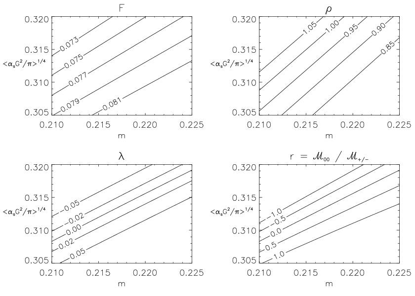
Concerning numerical predictions from our model, we have to stick to Eq. (66). The measured branching ratios for and are and , respectively [36]. In order to predict the experimental value solely with the mechanism considered in this section, we should have . Numerically, we use [32]. In previous papers on the heavy-light chiral quark model constituent masses 220 MeV and 315 MeV has been used. From the plot of in Fig. 3, we observe that the experimental value of can easily be accomodated by values of such orders. The bad news is that in our case the value of and thereby and is very sensitive to the explicit choice of and . Thus fine-tuning has to be used.
We also find that the perturbative anomaly tail will numerically reproduce the amplitude for , corresponding to a quark mass 11 MeV, i.e. of same order of magnitude as typical current quark masses. Using a hybrid description with a quark model with constituent quark masses for the colored current in (50)-(52), and the anomaly tail description [34, 35] for the colored current in (53), (54 and (55) is not preferrable. Also, such a hybrid description also fails to show the behaviour required by QCD-factorization. Still it might be interesting that we can numerically match the colored current for outgoing with the anomaly tail description. .
Note that there are also mesonic loop contributions similar to those contributing to processes of the type and [9, 11]. For those processes intermediate mesons contributed. In the present case the analogous contributions would involve energetic vector mesons , and we would need the amplitudes for . Such loops are shown in Fig. 4. The diagram to the right would be calculable within an extended theory involving energetic vector mesons. Unfortunately while the diagram to the left would be dubious because typical loop momenta would significantly exceed 1 GeV, and would require insertion of ad hoc form factors or should be handled within dispersion relation techniques. Both diagrams would of course require knowledge of the coupling in Fig. 4. In any case such calculations are beyond the scope of this paper.

VI Conclusion
We have pointed out that the factorized amplitude for process is proportional to a Wilson coefficient combination close to zero. Thus the nonfactorizable contributions dominate the amplitude for this decay mode. To handle the nonfactorizable contributions we have extended previous chiral quark models for the pure light quark case[24] used in [25, 23, 19], and the heavy light case[20] used in [6, 12, 9, 22, 11, 21], to include also energetic light quarks.
We have found that within our model we can account for the amplitude needed to explain the experimental branching ratio for [36]. In addition the ratio between the non-factorizable and factorized amplitude scales as in agreement with QCD factorization [1]. However, the bad news is that the calculated amplitude is very sensitive to our model-dependent parameters, i.e. the constituent quark mass , and the gluon condensate . Anyway, final state interactions should be present[37].
Acknowledgements.
JOE is supported in part by the Norwegian research council and in the beginning of this work, also by the European Commision RTN network, Contract No. MRTN-CT-2006-035482 (FLAVIAnet).References
- [1] M. Beneke, G. Buchalla, M. Neubert, C.T. Sachrajda, Phys. Rev. Lett. 83, 1914 (1999).
- [2] C.W. Bauer, S. Fleming, and M. Luke, Phys. Rev. D63, 014006 (2000). C.W. Bauer, S. Fleming, D. Pirjol, and I.W. Stewart, Phys. Rev. D63, 114020 (2001) C.W. Bauer, D. Pirjol, I. Z. Rothstein, I.W. Stewart, Phys. Rev. D70, 054015 (2004).
- [3] Y.Y. Keum, H-n. Li, A.I. Sanda, Phys. Lett. B504, 6-14 (2001). Ying Li, Ciai-Diam Lü, and Zhen-Jun Xiao, J. Phys. G31, 273 (1999).
- [4]
See for example: A. Khodjamirian, Th. Mannel, M. Melcher , and B. Melić
Phys. Rev. D72, 094012 (2009), - [5] See for instance M. Neubert, Phys. Rep. 245, 259 (1994). A.V. Manohar and M.B. Wise: heavy Quark Physics, Cambridge University Press, 2000
- [6] A. Hiorth and J.O. Eeg, Eur. Phys. J. direct C30, 006 (2003); and references therein.
- [7]
R. Casalbuoni, A. Deandrea, N. Di Bartolomeo,
R. Gatto, F. Feruglio and G. Nardulli,
Phys. Rep. 281, 145 (1997). - [8] C.G. Boyd and B. Grinstein, Nucl. Phys. B451, 177 (1995).
- [9]
J.O. Eeg, S. Fajfer , and A. Hiorth,
Phys.Lett. B570, 46-52 (2003);
J.O. Eeg, S. Fajfer, and A. Prapotnik, Eur. Phys. J. C42, 29-36 (2005).
See also: J.O. Eeg, S. Fajfer, J. Zupan, Phys. Rev. D64, 034010 (2001), and
J.O. Eeg, Acta Phys. Polon. B38 2869-2878 (2007). e-Print: arXiv:0704.0167 [hep-ph] - [10] B. Grinstein and R.F. Lebed, Phys. Rev. D60, 031302(R) (1999).
- [11] J.A. Macdonald Sørensen and J.O. Eeg, Phys. Rev. D75, 034015 (2007) hep-ph/0605078.
- [12] J.O. Eeg, A. Hiorth, and A.D. Polosa, Phys. Rev. D65, 054030 (2002).
- [13] Lars E. Leganger and Jan O. Eeg, Phys. Rev. D82 074007 (2010) arXiv:1003.3348 [hep-ph]
- [14] Lars E. Leganger, Master Thesis, Univ of Oslo, 2007.
- [15] M.J. Dougan and B. Grinstein, Phys. Lett. B252, 583 (1991)
- [16]
J. Charles, A. Le Yaouanc, L. Oliver, O. Pène and J.C. Raynal,
Phys. Rev. D60, 014001 (1999). - [17] C. Balzereit, T. Mannel, and W. Kilian, Phys. Rev. D58, 114029 (1998). U. Aglietti and G: Corbò, Int. J. Mod. Phys. A15, 363 (2000).
- [18]
See for instance : M. Beneke, T. Huber and Xin-Qiang Li,
Nucl. Phys. B832, 109-151 (2010) and references therein.
See also ref. [4], and
H.-n. Li and S. Mishima, arXiv:0901.1272 [hep-ph], and references therein. - [19]
S. Bertolini, J.O. Eeg and M. Fabbrichesi,
Nucl. Phys. B449, 197 (1995);
V. Antonelli, S. Bertolini, J.O. Eeg, M. Fabbrichesi and E.I. Lashin,
Nucl. Phys. B469, 143 (1996); S. Bertolini, J.O. Eeg, M. Fabbrichesi and E.I. Lashin,
Nucl. Phys. B514, 63 (1998); ibid B514, 93 (1998). - [20] A. Hiorth and J.O. Eeg, Phys. Rev. D66, 074001 (2002).
- [21] J.O. Eeg and A. Hiorth, Fizika B14, 41-74 (2005). e-Print: hep-ph/0411393
- [22] A. Hiorth and J. O. Eeg, Eur. Phys. J. direct C39 S1, 27-35 (2005), hep-ph/0304247.
- [23]
J.O. Eeg and I. Picek, Phys. Lett. B301, 423 (1993);
ibid. B323 193 (1994);
A.E. Bergan and J.O. Eeg, Phys. Lett. B390, 420 (1997). - [24]
See for example:
A. Manohar and H. Georgi, Nucl. Phys. B234, 189 (1984);
D. Espriu, E. de Rafael and J. Taron, Nucl. Phys. B345, 22 (1990); and references therein. - [25] A. Pich and E. de Rafael, Nucl. Phys. B358, 311 (1991).
- [26]
W.A. Bardeen and C.T. Hill, Phys. Rev. D49, 409 (1994);
A. Deandrea, N. Di Bartolomeo, R. Gatto, G. Nardulli, and A.D. Polosa,
Phys. Rev. D58, 034004 (1998); A.D. Polosa, Riv. Nuovo Cim. 23 N11, 1 (2000);
D. Ebert, T. Feldmann R. Friedrich and H. Reinhardt, Nucl. Phys. B434, 619 (1995). - [27]
A.A. Andrianov and V.A. Andrianov, Z. Phys. C55 435 (1992);
J. Bijnens, E. de Rafael, and H. Zheng, Z. Phys. C62 437 (1994). - [28] B. Grinstein and D. Pirjol, Phys. Lett. B615, 213-220 (2005). e-Print: hep-ph/0501237.
- [29]
M.K. Gaillard and B.W. Lee, Phys. Rev. Lett. 33, 108 (1974)
G. Altarelli and L. Maiani, Phys.Lett. 52 B, 351 (1974).
A.I. Vainstein, V.I. Zakharov, and M. A. Shifman,
Zh. Exp. Theor. Fiz. 72 1275 (1977)
(Sov. Phys. JETP 45 670-682 (1977) ) . G. Buchalla, A.J. Buras and M.E. Lautenbacher, Rev. Mod. Phys. 68, 1125 (1996),
e-Print: hep-ph/9512380, and references therein. M. Ciuchini, E. Franco, G. Martinelli, and L. Reina, Nucl.Phys. B415, 403 (1994).
e-Print: hep-ph/9304257. See also:
B. Grinstein, W. Kilian, T. Mannel, and M.B. Wise, Nucl. Phys. B363 , 19 (1991),
R. Fleischer, Nucl. Phys. B412, 201 (1994). - [30]
V. Novikov, A.I. Vainstein, V.I. Zakharov, and M. A. Shifman,
Fortschr. Phys. 32 No 11, 585-622 (1984). - [31] K.Kumerički and J.O. Eeg, Phys. Rev. D81, 074015 (2010); arXiv:0910.5428 [hep-ph].
- [32]
See for example:
P. Ball, JHEP 9809:005 (1998)
F. De Fazio, T. Feldman,and T. Hurth, JHEP 0802:031 (2008). - [33] L.J. Reinders, H. Rubinstein and S. Yazaki, Phys. Rep. 127, 1 (1985).
- [34] T.N. Pham and X.Y. Pham, Phys. Lett. B247 , 438 (1990)
- [35] J.O.Eeg, K. Kumerički, and I. Picek, Phys. Lett. B563 , 87 (2003).
- [36] Amsler,C. et. al. (Particle Data Group), Phys. Lett. B 667 1
- [37] A.B. Kaidalov and M.I. Vysotsky, Phys. Atom. Nucl.70, 712-721 (2007). (hep-ph/0603013)