Polarized currents in Coulomb blockade and Kondo regimes without magnetic fields

Anh T. Ngo Affiliation: Department of Physics and Astronomy, and Nanoscale and Quantum Phenomena Institute, Ohio University, Athens, Ohio 45701-2979 Edson Vernek Affiliation: Department of Physics and Astronomy, and Nanoscale and Quantum Phenomena Institute, Ohio University, Athens, Ohio 45701-2979 Affiliation: Instituto de Física - Universidade Federal de Uberlândia, Uberlândia, MG 38400-902, Brazil Sergio E. Ulloa Affiliation: Department of Physics and Astronomy, and Nanoscale and Quantum Phenomena Institute, Ohio University, Athens, Ohio 45701-2979

August 24, 2026

Abstract

We present studies of the Coulomb blockade and Kondo regimes of transport through a quantum dot connected to current leads through spin-polarizing quantum point contacts (QPCs). This structure, arising from the effect of lateral spin-orbit fields defining the QPCs, results in spin-polarized currents even in the absence of external magnetic fields and greatly affects the correlations in the dot. Using equation-of-motion and numerical renormalization group calculations we obtain the conductance and spin polarization for this system under different parameter regimes. We find that the system exhibits spin-polarized conductance in both the Coulomb blockade and Kondo regimes, all in the absence of applied magnetic fields. We analyze the role that the spin-dependent tunneling amplitudes of the QPC play in determining the charge and net magnetic moment in the dot. These effects, controllable by lateral gate voltages, may provide an alternative approach for exploring Kondo correlations, as well as possible spin devices.

pacs

72.15.Qm, 72.25.-b, 72.10.-d, 73.23.Hk

I Introduction

Electronic transport in semiconducting nanostructures is studied both as it has great potential applications in spintronics, [1] and because of its exquisite control of parameters, which allow insightful probes into fundamental physical phenomena. Electrons in such systems experience externally controlled confining environments that result in strong Coulomb interactions with other electrons. As such, quantum dot (QD) structures provide well-characterized and defined systems for studying quantum many-body physics. QDs may also allow the realization of solid state quantum computation devices as well as spintronic semiconductor devices with unprecedented functionalities. [2]

Manipulation of spin-polarized current sources is crucial in spintronics. This typically requires efficient spin injection into conventional semiconductors. The difficulties with spin injection from ferromagnetic metal leads has stimulated extensive efforts to produce spin polarized currents out of unpolarized sources. [3] In this context, the Rashba spin-orbit (RSO) coupling mechanism provides a basis for possible device applications. [4] This coupling, arising from interfacial structure asymmetries, depends on the materials used as well as on the confinement geometry of the structures. [5, 6] Most interestingly, the Rashba effect allows external tunability, which has been studied experimentally in QDs [7] and quantum point contacts. [8, 9]

In this paper we study the electronic transport through a quantum dot connected to polarizing quantum point contacts (QPCs) in both the Coulomb blockade (CB) and Kondo regimes. Due to strong spin-orbit interactions, [9, 6] QPCs can exhibit spin-dependent hybridization of the QD states with the leads, without applied magnetic fields, opening the possibility for generating spin-polarized transport in an all-electrical setup. These effects are controllable by lateral gate voltages applied on QPCs, resulting in spatially asymmetric structures, as in recent experiments.[9] Using the equation-of-motion technique and numerical renormalization group (NRG) calculations we obtain the electronic Green’s function, conductance and spin polarization in different system regimes. Our results show that both the CB and Kondo regimes exhibit non-zero spin-polarized conductance in this system. We analyze how the spin-dependent hybridization of the QPC modifies the charge accumulation in the dot, as well as the density of states (spectral functions) of the system. Interestingly, we find that the polarizing QPCs produce spin polarization and split DOS in the Kondo regime akin to that reported for current injection from ferromagnetic leads, [10] although here it occurs for unpolarized reservoirs. Our theoretical studies suggest that these effects could be accessible in experiments and result in future spintronic devices.

The paper is organized as follows. First, we present the main features of the current polarization in quantum point contact systems with lateral spin-orbit, obtained by scattering matrix methods in section II. The next section describes the model of a quantum dot connected to current leads via polarizing QPCs. In section III.1 we use the equation-of-motion (EOM) technique to obtain the dot Green’s function and discuss numerical results in both the CB and Kondo regimes. In section III.2 we revisit the problem using the numerical renormalization group approach, which provides the most reliable information in the Kondo regime for realistic system parameters. The paper concludes with final remarks and summary in section IV.

II Polarizing QPC

The effective electric field in the $z$ direction that creates a two-dimensional electron gas (2DEG) confined to the $x$ - $y$ plane results in the well-known Rashba spin orbit interaction, [4, 5]

\displaystyle H_{SO}^{R}=\frac{\alpha}{\hbar}\left(\sigma_{x}P_{y}-\sigma_{y}P_{x}\right).

(1)

Here, $\sigma_{x}$ and $\sigma_{y}$ are Pauli matrices, and $\alpha$ is Rashba spin orbit coupling constant, which is proportional to the field and is therefore material and structure dependent. Electrons on this 2DEG entering a quantum dot, pass through QPCs defined via a confining potential $V(x,y)$ which can be thought as made of two parts: $U(y)+V_{b}(x,y)$ , where $U(y)$ defines a hard-wall potential of width $W$ (related in the experiment to the side-wall etching defining the structure) outlining the overall channel structure, while $V_{b}(x,y)$ is the potential generating the QPC barrier, and effectively modulated by the side gate potentials of the structure. [9] We model such barrier by [11]

\displaystyle V_{b}(x,y)=\frac{1}{2}V_{g}\left(1+\cos\frac{\pi x}{L_{x}}\right)+\frac{1}{2}m\omega^{2}\bar{y}^{2}\Theta(\bar{y})

(2)

with $\bar{y}=y-y_{s}$ , and

\displaystyle y_{s}=W_{1}\left(1-\cos\frac{\pi x}{L_{x}}\right)\,,

(3)

where $\Theta(x)$ is the step function, $m$ is the effective mass of the electrons, $L_{x}$ is the unit length of the structure in the $x$ direction (along the current direction) and $\omega$ is the confinement potential frequency. Notice that this potential form is asymmetric in the $y$ direction, to reflect an essential ingredient in the experiments: the QPC potential must lack $y$ -reflection symmetry in order to generate the polarizing effect along the $z$ -direction. [11, 12, 13] In fact, the fields forming $V_{b}$ generate a spin-orbit coupling given by [5]

\displaystyle V_{SO}^{\beta}=-\frac{\beta}{\hbar}\nabla V_{b}\cdot(\mathbf{\hat{\sigma}}\times\mathbf{\hat{P}}),

(4)

where $\beta$ is material-specific. Notice that $\nabla V_{b}$ lies in the $x$ - $y$ plane, so that the barrier fields induce a lateral spin-orbit coupling. The total Hamiltonian of the QPC will then be given by,

\displaystyle H=\frac{P_{x}^{2}+P_{y}^{2}}{2m}+H_{SO}^{R}+V(x,y)+V_{SO}^{\beta}.

(5)

Refer to caption — Figure 1: (color online) Total and spin-dependent conductances for an asymmetric QPC as function of Rashba spin-orbit coupling $\alpha$ , obtained from a scattering matrix approach.[6] The interplay of vertical and lateral SO effects may result in large asymmetry for the up and down spin components for realistic structure parameters, even in the tunneling regime shown here ( $G_{\sigma}\ll 1$ ).

Using a scattering-matrix formalism to study the spin-dependent electron transport in this QPC, [14, 6] we find that a net spin-polarized conductance is produced only for $y$ -asymmetric potentials. [6] We can calculate the conductance of the structure, assuming that the SO coupling $\alpha$ and $V(x,y)$ are zero at the source and drain 2DEG reservoirs, while both of these terms in the Hamiltonian are turned on in the QPC region. Typical structure parameters in experiments can be cast in terms of characteristic length and energy scales, $L_{0}=32.5$ nm, and $E_{0}=3.12$ meV, with $\alpha_{0}=E_{0}L_{0}=1.0\times 10^{-12}$ eVm, a typical value of spin-orbit coupling. Using $W=L_{x}=2L_{0}$ and $W_{1}=0.6L_{0}$ as width/length of the confining potential, with $\omega=6\times 10^{13}$ s^-1, and $\beta=0.97\times 10^{-16}$ m², gives results as shown in Fig. 1. This figure shows spin-dependent conductances as functions of Rashba coupling $\alpha$ , for a potential barrier which is near its conduction onset (or “pinch-off”, as controlled by the value of $V_{g}$ ); arrows indicate the results of spin up and down conductances. We see that conductances $G_{\uparrow}$ and $G_{\downarrow}$ can be very different from each other, even in the tunneling regime (where each $G_{\sigma}\ll 1$ ) in which the QPC would operate to create a quantum dot in the 2DEG. We stress that for these realistic values of structure parameters, one obtains non-zero spin polarization even when there is no external magnetic field and the injection is unpolarized. This interesting result can be understood from anticrossing features in the subband energy structure in the channel region defining the QPC. [9, 6] The spin mixings and avoided crossings generate spin rotation as electrons pass through the narrow constriction of the QPC, and can generate large values of the ratio $G_{\uparrow}/G_{\downarrow}$ , even in the tunneling regime. Two of these QPCs can then be used to define the QD and result in interesting charging and conductance regimes, as we will see below.

III Quantum dot with polarizing QPCs

In order to address the transport through a quantum dot formed with polarizing QPCs, we consider the single impurity Anderson model given by the following Hamiltonian:

	$\displaystyle H=\sum_{\ell k\sigma}\varepsilon_{\ell k}c^{\dagger}_{\ell k\sigma}c_{\ell k\sigma}+\sum_{\sigma}\varepsilon_{d}c^{\dagger}_{d\sigma}c_{d\sigma}+Un_{d\uparrow}n_{d\downarrow}$
	$\displaystyle+\sum_{\ell k\sigma}t_{\sigma}(c^{\dagger}_{d\sigma}c_{\ell k\sigma}+c^{\dagger}_{\ell k\sigma}c_{d\sigma}),$		(6)

where $c^{\dagger}_{d\sigma}(c_{d\sigma})$ is the creation (annihilation) operator of an electron of spin $\sigma$ in the dot. The quantities $\varepsilon_{\ell k}$ , $\varepsilon_{d}$ are the energies of the electrons in the $\ell^{\it th}$ conduction band channels ( $\ell=L,R$ ) and the single local energy level in the dot, respectively. $U$ is the Coulomb repulsion between electrons occupying the QD with $n_{d\sigma}=c^{\dagger}_{d\sigma}c_{d\sigma}$ , while $t_{\sigma}$ represents the lead-QD hybridization occurring via tunneling through the QPC, and which is assumed to be $k$ -independent. The density of states for conduction electrons in each lead is taken to be constant, $\rho_{L}(\varepsilon)=\rho_{R}(\varepsilon)\equiv\rho=(1/2D)\Theta(D-|\varepsilon|)$ , where $D$ is the conduction band halfwidth (hereafter taken as our energy unity).

The theoretical description of such quantum dot system, especially in the strong correlations regime, has been greatly developed over the years. [15] Techniques of note include quantum Monte-Carlo, [16] equations of motion for the Green’s functions,[17] and the numerical renormalization group approach.[18] In what follows, we explore the role that SO interactions play on the Coulomb blockade and Kondo regimes of transport of the QD, utilizing equations of motion and numerical renormalization group formalisms.

III.1 Equation of motion approach and numerical results

To calculate the charge and conductance of the system we calculate Green’s functions (GFs), which allow us to take into account the correlations induced by the Coulomb interaction in the QD. The retarded double-time Green’s functions are defined as ( $\hbar=1$ )[19]

i\langle\langle A;B\rangle\rangle=\int_{-\infty}^{\infty}\langle[A(\tau),B(0)]_{+}\rangle\Theta(\tau)e^{-i\omega\tau}d\tau,

(7)

where $A$ and $B$ are generic fermionic operators, $[A,B]_{+}$ indicates their anticommutator and $\langle\cdots\rangle$ indicates the thermodynamic average for $T>0$ , or the ground state expectation value for $T=0$ . The GF can be obtained using equation of motion (EOM) techniques, so that

\displaystyle\omega\langle\langle A;B\rangle\rangle=\langle[A,B]_{+}\rangle+\langle\langle[A,H];B\rangle\rangle,

(8)

where $[A,B]$ represents a commutator. Iteration of this formula generates a hierarchy of expressions, starting with the local one-particle GF as

\left(\omega-\varepsilon_{d}-\sum_{k}\frac{\tilde{t}_{\sigma}^{2}}{\omega-\varepsilon_{k}}\right)\langle\langle c_{d\sigma};c^{\dagger}_{d\sigma}\rangle\rangle=1+U\langle\langle c_{d\sigma}n_{d\bar{\sigma}};c^{\dagger}_{d\sigma}\rangle\rangle,

(9)

where $\tilde{t}_{\sigma}=\sqrt{2}t_{\sigma}$ and $\bar{\sigma}=-\sigma$ . The new (higher order) GF on the right hand side of Eq. (9) can also be determined from (8), giving

\displaystyle(\omega-\varepsilon_{d}-U)\langle\langle c_{d\sigma}n_{d\bar{\sigma}};c^{\dagger}_{d\sigma}\rangle\rangle=\langle n_{d\bar{\sigma}}\rangle+\tilde{t}_{\sigma}\sum_{k}\left(\langle\langle c_{k\sigma}n_{d\bar{\sigma}};c^{\dagger}_{d\sigma}\rangle\rangle-\langle\langle c_{k\bar{\sigma}}c^{\dagger}_{d\bar{\sigma}}c_{d\sigma};c^{\dagger}_{d\sigma}\rangle\rangle+\langle\langle c^{\dagger}_{k\bar{\sigma}}c_{d\bar{\sigma}}c_{d\sigma};c^{\dagger}_{d\sigma}\rangle\rangle\right).

(10)

III.1.1 Coulomb blockade regime

Although the EOM in Eq. (10) is exact, a solution of the impurity GF requires a procedure to truncate and/or decouple the higher order terms appearing on the right hand side of (10). A solution that captures the Coulomb blockade physics is given by the Hubbard-I approximation:[20]

$\displaystyle\langle\langle c_{k\sigma}n_{d\bar{\sigma}};c^{\dagger}_{d\sigma}\rangle\rangle$	$\displaystyle\simeq$	$\displaystyle\langle n_{d\bar{\sigma}}\rangle\langle\langle c_{k\sigma};c^{\dagger}_{d\sigma}\rangle\rangle$
$\displaystyle\langle\langle c_{k\bar{\sigma}}c^{\dagger}_{d\bar{\sigma}}c_{d\sigma};c^{\dagger}_{d\sigma}\rangle\rangle$	$\displaystyle\simeq$	$\displaystyle\langle c_{k\bar{\sigma}}c^{\dagger}_{d\bar{\sigma}}\rangle\langle\langle c_{k\sigma};c^{\dagger}_{d\sigma}\rangle\rangle$
$\displaystyle\langle\langle c^{\dagger}_{k\bar{\sigma}}c_{d\bar{\sigma}}c_{d\sigma};c^{\dagger}_{d\sigma}\rangle\rangle$	$\displaystyle\simeq$	$\displaystyle\langle c^{\dagger}_{k\bar{\sigma}}c_{d\bar{\sigma}}\rangle\langle\langle c_{k\sigma};c^{\dagger}_{d\sigma}\rangle\rangle,$	(11)

which allows one to write

\displaystyle G_{d\sigma}(\omega)\equiv\langle\langle c_{d\sigma};c^{\dagger}_{d\sigma}\rangle\rangle_{\omega}=\frac{G^{0}_{d\sigma}(\omega)}{1-G^{0}_{d\sigma}(\omega)\tilde{t}^{2}_{\sigma}\tilde{g}(\omega)},

(12)

where $G^{0}_{d\sigma}(\omega)=\frac{1-\langle n_{d\bar{\sigma}}\rangle}{\omega-\varepsilon_{d}}+\frac{\langle n_{d\bar{\sigma}}\rangle}{\omega-\varepsilon_{d}-U}$ is the local GF in the “atomic” approximation (the exact result for $t_{\sigma}=0$ ), and $\tilde{g}(\omega)=\sum_{k}(\omega-\epsilon_{k})^{-1}$ is the non-interacting GF of the leads. The DOS of the system (proportional to the imaginary part of $G_{d\sigma}$ ) contains two Hubbard peaks of width proportional to $\Gamma_{\sigma}=\pi t^{2}_{\sigma}/D$ , resulting in the broadening of the poles of $G^{0}_{d\sigma}$ . The spectral weights of these peaks are controlled by the dot level occupancy with opposite spin, and caused by the Coulomb interaction in the dot. Notice that the SO-induced polarization of the QPC results in different peak widths for the different spins. The Hubbard-I approximation (11) is known to be valid for a large $U/\Gamma$ ratio, when the Hubbard subbands are well separated in energy scale. [15] It is the simplest scheme which describes correlated electrons, although, since it ignores the Kondo effect, it is a reasonable description only at temperatures higher than the Kondo scale ( $T\gg T_{K}$ –see next section).

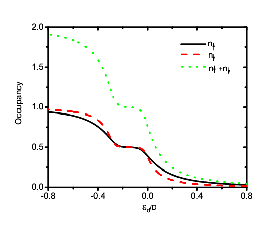
The occupancies of spin $\uparrow$ and $\downarrow$ are calculated self-consistently from the equation

\displaystyle\langle n_{d\sigma}\rangle=\int f(\omega)\left(-\frac{1}{\pi}\text{Im}\left[G_{d\sigma}(\omega)\right]\right)d\omega\,,

(13)

where $f(\omega)$ is the Fermi function. It is clear that when the QPCs are not polarizing, $t_{\uparrow}=t_{\downarrow}$ , the occupancy curves for spin-up and down coincide and a plateau of width $\sim U$ appears when the QD level moves below the Fermi level ( $\varepsilon_{d}+U\gtrsim E_{F}\gtrsim\varepsilon_{d}$ ). This situation changes when the QPCs are polarized (see Fig. 2), as the different $t_{\sigma}$ result in $\Gamma_{\uparrow}\neq\Gamma_{\downarrow}$ , which in turn produce different $\langle n_{d\uparrow}\rangle$ and $\langle n_{d\downarrow}\rangle$ , especially on both sides of the plateau.

The zero-bias conductance is calculated using a Landauer formula generalized for interacting systems [21]

\displaystyle G_{\sigma}=\frac{e^{2}}{h}\Gamma_{\sigma}\int d\epsilon\frac{\partial f(\epsilon)}{\partial\epsilon}\,\text{Im}[G_{d\sigma}(\epsilon)],

(14)

for symmetric coupling of the leads for each spin. One can also calculate the polarization factor

\displaystyle\eta=\frac{G_{\uparrow}-G_{\downarrow}}{G_{\uparrow}+G_{\downarrow}},

(15)

which gives a measure of current polarization in the system. Figure 3 shows the spin-dependent conductances and polarization for the system in the Hubbard-I approximation. As $\langle n_{d\uparrow}\rangle\neq\langle n_{d\downarrow}\rangle$ in general (except at the particle-hole symmetry point, $\varepsilon_{d}=-U/2$ ), the conductance per spin $G_{\sigma}$ are also different. Notice that the spin-dependent conductance peaks are very asymmetric and non-Lorentzian, due to the peculiar behavior of the occupancies and their different up and down-spin couplings. As we consider here the case $\Gamma_{\uparrow}>\Gamma_{\downarrow}$ , one clearly sees that generally $G_{\uparrow}>G_{\downarrow}$ over the entire range of $\varepsilon_{d}$ values. As a consequence, there is a net up-spin polarization ( $\simeq 60$ %) and conductance around the resonant peaks, with the latter reaching $\simeq 0.3(e^{2}/h)$ .

III.1.2 Kondo regime

To study the low-temperature behavior of the system within the EOM we need to consider higher order GFs in Eq. (10). Using Lacroix’s approach, [17] one can obtain relations for the three GFs on the right side of (10) as:

	$\displaystyle(\omega-\varepsilon_{k\sigma})\langle\langle c_{k\sigma}n_{d\bar{\sigma}};c^{\dagger}_{d\sigma}\rangle\rangle$	$\displaystyle=$	$\displaystyle\langle[c_{k\sigma}n_{d\bar{\sigma}};c^{\dagger}_{d\sigma}]_{+}\rangle+\langle\langle[c_{k\sigma}n_{d\bar{\sigma}};H];c^{\dagger}_{d\sigma}\rangle\rangle$		(16)
		$\displaystyle=$	$\displaystyle\tilde{t}_{\sigma}\langle\langle n_{d\bar{\sigma}}c_{d\sigma};c^{\dagger}_{d\sigma}\rangle\rangle+\tilde{t}_{\bar{\sigma}}\sum_{k^{\prime}}[\langle\langle c_{k\sigma}c^{\dagger}_{d\bar{\sigma}}c_{k^{\prime}\bar{\sigma}};c^{\dagger}_{d\sigma}\rangle\rangle-\langle\langle c^{\dagger}_{k^{\prime}\bar{\sigma}}c_{d\bar{\sigma}}c_{k\sigma};c^{\dagger}_{d\sigma}\rangle\rangle],$		(16)

$\displaystyle(\omega-\varepsilon_{d\sigma}+\varepsilon_{d\bar{\sigma}}-\varepsilon_{k\bar{\sigma}})\langle\langle c_{k\bar{\sigma}}c^{\dagger}_{d\bar{\sigma}}c_{d\sigma};c^{\dagger}_{d\sigma}\rangle\rangle$	$\displaystyle=\langle[c^{\dagger}_{d\bar{\sigma}}c_{k\bar{\sigma}}c_{d\sigma};c^{\dagger}_{d\sigma}]_{+}\rangle+\langle\langle[c^{\dagger}_{d\bar{\sigma}}c_{k\bar{\sigma}}c_{d\sigma};H];c^{\dagger}_{d\sigma}\rangle\rangle$	(17)
	$\displaystyle=\langle c^{\dagger}_{d\bar{\sigma}}c_{k\bar{\sigma}}\rangle+\tilde{t}_{\bar{\sigma}}\langle\langle n_{d\bar{\sigma}}c_{d\sigma};c^{\dagger}_{d\sigma}\rangle\rangle+\sum_{k^{\prime}}[-\tilde{t}_{\bar{\sigma}}\langle\langle c^{\dagger}_{k^{\prime}\bar{\sigma}}c_{k\bar{\sigma}}c_{d\sigma};c^{\dagger}_{d\sigma}\rangle\rangle$
	$\displaystyle+\tilde{t}_{\sigma}\langle\langle c^{\dagger}_{d\bar{\sigma}}c_{k\bar{\sigma}}c_{k^{\prime}\sigma};c^{\dagger}_{d\sigma}\rangle\rangle],$

and

$\displaystyle(\omega-\varepsilon_{d\sigma}-\varepsilon_{d\bar{\sigma}}+\varepsilon_{k\bar{\sigma}}-U)\langle\langle c^{\dagger}_{k\bar{\sigma}}c_{d\bar{\sigma}}c_{d\sigma};c^{\dagger}_{d\sigma}\rangle\rangle$	$\displaystyle=\langle[c^{\dagger}_{k\bar{\sigma}}c_{d\bar{\sigma}}c_{d\sigma};c^{\dagger}_{d\sigma}]_{+}\rangle+\langle\langle[c^{\dagger}_{k\bar{\sigma}}c_{d\bar{\sigma}}c_{d\sigma};H];c^{\dagger}_{d\sigma}\rangle\rangle$	(18)
	$\displaystyle=\langle c^{\dagger}_{k\bar{\sigma}}c_{d\bar{\sigma}}\rangle-\tilde{t}_{\bar{\sigma}}\langle\langle n_{d\bar{\sigma}}c_{d\sigma};c^{\dagger}_{d\sigma}\rangle\rangle+\sum_{k^{\prime}}[\tilde{t}_{\sigma}\langle\langle c^{\dagger}_{k^{\prime}\bar{\sigma}}c_{d\bar{\sigma}}c_{k^{\prime}\sigma};c^{\dagger}_{d\sigma}\rangle\rangle$
	$\displaystyle-\tilde{t}_{\bar{\sigma}}\langle\langle c^{\dagger}_{k\bar{\sigma}}c_{d\sigma}c_{k^{\prime}\bar{\sigma}};c^{\dagger}_{d\sigma}\rangle\rangle].$

Following the decoupling procedure in Ref. 17, each GF of the type $\langle\langle A^{*}BC,D^{*}\rangle\rangle$ is replaced by

\displaystyle\approx\langle A^{*}B\rangle\langle\langle C,D^{*}\rangle\rangle-\langle A^{*}C\rangle\langle\langle B,D^{*}\rangle\rangle,

(19)

resulting in an equation for the dot GF given by

	$\displaystyle G_{d\sigma}(\omega)$	$\displaystyle=$	$\displaystyle\left[U(\omega)-\langle n_{d\bar{\sigma}}\rangle-B_{\bar{\sigma}}(\omega)-B_{\bar{\sigma}}(\omega_{1})\right]$		(20)
			$\displaystyle\times\left\{U(\omega)[\omega-\varepsilon_{d\sigma}-\Sigma_{\sigma}(\omega)]+[B_{\bar{\sigma}}(\omega)+B_{\bar{\sigma}}(\omega_{1})\right]\Sigma_{\sigma}(\omega)-A_{\bar{\sigma}}(\omega)+A_{\bar{\sigma}}(\omega_{1})\}^{-1}\,,$		(20)

where $\Sigma_{\sigma}(x)=\sum_{k}|\tilde{t}_{\sigma}|^{2}/(x-\varepsilon_{k\sigma})$ , $U(\omega)=[U-\omega+\varepsilon_{d\sigma}-\Sigma_{\sigma}(\omega)+\Sigma_{\bar{\sigma}}(\omega)-\Sigma_{\bar{\sigma}}(\omega_{1})]/U$ and $\omega_{1}=-\omega+\varepsilon_{d\sigma}+U$ . The functions $A_{\sigma}(\omega)$ and $B_{\sigma}(\omega)$ are given by

	$\displaystyle B_{\sigma}(\omega)$	$\displaystyle=$	$\displaystyle\frac{i}{2\pi}\int d\omega^{\prime}f(\omega^{\prime})\left[G_{d\sigma}(\omega^{\prime})\frac{\Sigma_{\sigma}(\omega^{\prime})-\Sigma_{\sigma}(\omega)}{\omega-\omega^{\prime}-i\delta}-G^{}_{d\sigma}(\omega^{\prime})\frac{\Sigma^{}_{\sigma}(\omega^{\prime})-\Sigma_{\sigma}(\omega)}{\omega-\omega^{\prime}+i\delta}\right]$
	$\displaystyle A_{\sigma}(\omega)$	$\displaystyle=$	$\displaystyle\frac{i}{2\pi}\int d\omega^{\prime}f(\omega^{\prime})\left[\left(1+G_{d\sigma}(\omega^{\prime})\Sigma_{\sigma}(\omega^{\prime})\right)\frac{\Sigma_{\sigma}(\omega^{\prime})-\Sigma_{\sigma}(\omega)}{\omega-\omega^{\prime}-i\delta}-\left(1+G^{}_{d\sigma}(\omega^{\prime})\Sigma^{}_{\sigma}(\omega^{\prime})\right)\frac{\Sigma^{*}_{\sigma}(\omega^{\prime})-\Sigma_{\sigma}(\omega)}{\omega-\omega^{\prime}+i\delta}\right],$		(21)

and have to be calculated self-consistently. In the limit $U\rightarrow\infty$ , the GF (20) acquires a simpler form,

\displaystyle G_{d\sigma}(\omega)=\frac{1-\langle n_{d\bar{\sigma}}\rangle-B_{\bar{\sigma}}(\omega)}{\omega-\varepsilon_{d\sigma}-(1-B_{\bar{\sigma}}(\omega))\Sigma_{\sigma}(\omega)-A_{\bar{\sigma}}(\omega)}.

(22)

In the following, we solve numerically for the spectral function (DOS) in the Kondo regime by the self-consistent iteration of Eqs. (13) and (22). Figure 4 shows the DOS vs. $\omega$ at low temperature ( $T=10^{-7}$ ) for both spin orientations (and total), when the QD electron level $\varepsilon_{d}$ is taken to be at $-0.136$ . The three curves exhibit Kondo resonance peaks near the Fermi level ( $\omega\simeq 0$ ), in addition to a much broader peak at $\omega\simeq\varepsilon_{d}$ . [17] Since the hybridization between leads and QD are spin dependent in this case, the DOS clearly splits into two different components for spin up and down. The DOS for spin down is shifted upwards in energy with respect to the spin up component, resulting in a lower occupancy for the down spin. Figure 5 shows indeed the occupancy curves for $\langle n_{d\uparrow}\rangle$ , $\langle n_{d\downarrow}\rangle$ and total $\langle n\rangle$ vs. $\varepsilon_{d}$ at a given temperature ( $T=10^{-7}$ ). Qualitatively similar to the results in the Coulomb blockade regime, the occupancy curves show that $\langle n_{d\uparrow}\rangle>\langle n_{d\downarrow}\rangle$ for $\omega\gtrsim-0.05$ , while the relation is reversed for smaller $\omega$ values, reflecting the asymmetry introduced by the polarizing QPCs, through $\Gamma_{\uparrow}$ and $\Gamma_{\downarrow}$ . Notice also that the plateaus at 0.5 are not as well defined here, due to the enhanced spin and charge fluctuations in the Kondo regime. The spin-orbit effect can be understood qualitatively as arising from a shift in the dot level (as well as depending on the occupancy factors): since the effective level position of the electron with spin $\sigma$ is given by $\varepsilon_{d\sigma}\approx\varepsilon_{d}+\text{Re}\Sigma^{{}^{\prime}}_{\sigma}(\omega)$ , where $\Sigma^{{}^{\prime}}_{\sigma}(\omega)\propto t_{\sigma}^{2}$ is the self-energy, and thus naturally causes the spin-dependent occupancy seen in the figure.

Figure 6(a) shows the spin-dependent conductance curves $G_{\sigma}$ vs. $\varepsilon_{d}$ . Several features are noteworthy. As $\varepsilon_{d}$ changes, the spin-dependent conductances exhibit the anticipated peaks at low temperature, with spin up conductance dominating (naturally, as $\Gamma_{\uparrow}>\Gamma_{\downarrow}$ ). Figure 6(b) shows the difference between spin up and down conductances as well as the spin polarization vs. $\varepsilon_{d}$ . In this regime, the difference between the conductance for the two spin orientations reaches $\simeq 0.4(e^{2}/h)$ . Correspondingly, the net spin polarization reaches $\eta\simeq 60$ %.

Let us now analyze in more detail the effect of temperature on the conductance of the system and especially its drop for $\varepsilon_{d}\ll 0$ . The conductance curves in Fig. 6(a) are highly asymmetric about the Fermi energy and vanish rapidly away from it. This vanishing for very negative values of $\varepsilon_{d}$ is due to the the Kondo temperature, $T_{K}$ , becoming smaller than the temperature of the system. Figure 7 presents the total zero bias conductance as function of $\varepsilon_{d}$ for several values of temperature. As $T$ is lowered, the total conductance increases for a given $\varepsilon_{d}$ , and the width of the conductance peak increases in $\varepsilon_{d}$ . This explicitly reflects the existence of the Kondo resonant peak in the spectral function, and how the system will reach the unitary limit of conductance for $T=0$ for $\varepsilon_{d}$ well below the Fermi level.

Our discussions above are applied to the case of infinite $U$ , where the EOM method gives qualitatively accurate results in the Kondo regime. Extension of this approach for finite $U$ is known to be problematic, including its failure to exhibit a Kondo resonance at the particle-hole symmetry point ( $\varepsilon_{d}=-U/2$ ). [22] To carry out our study in the finite $U$ case, we use instead the essentially exact numerical renormalization group approach, as we discuss in the following section.

III.2 NRG results for finite U

For the finite- $U$ case we study the spin polarized conductance using the standard numerical renormalization group approach.[23, 18] In this case, unlike the previous infinite- $U$ case, the processes involving double occupied states are naturally present in the dynamics of the system, and allow for a reliable description of the low-energy behavior. We set $U=0.5$ and $T=0$ . Figure 8 depicts the local density of states calculated with NRG for the same system parameters as before, $\Gamma_{\uparrow}=0.06$ , $\Gamma_{\downarrow}=0.03$ , and with $\epsilon_{d}=-0.2$ . This value of $\epsilon_{d}$ corresponds to a situation where the system is away from the particle-hole symmetric point ( $=-U/2$ ), more suitable to compare to the previous infinite- $U$ calculation (where the system never reaches the p-h symmetry point). Notice that there is a strong spin asymmetry in the DOS; on the negative side of the $\omega$ -axis, the DOS for spin up (solid curve) presents a peak near $-0.2$ , corresponding to the energy of the local bare orbital $\varepsilon_{d}$ , slightly shifted by the real part of the proper self-energy. On the positive side of the $\omega$ -axis, the peak near $\epsilon_{d}+U$ would result in the succeeding CB peak, which appears only for the spin-down DOS (dashed curve). In this regime as well, the fact that $\Gamma_{\uparrow}>\Gamma_{\downarrow}$ favors the spin-up occupancy to the detriment of the spin-down occupancy. One also notices the important peaks close to the Fermi level, signature of the Kondo effect, which are slightly split away and suppressed by a seemingly effective magnetic field induced by the spin-asymmetric coupling to the leads. This phenomenon is akin to the suppression discussed by Martinek et al.,[10] in the context of a QD coupled to ferromagnetic leads. Notice, however, that no external magnetization is present in our system and that the polarization is only arising from the QPCs and due to the lateral SO interaction.

Analogously to the infinite- $U$ case, the spin-asymmetry discussed above induces spin polarized transport in the system. In Fig. 9 we show the conductance as a function of $\varepsilon_{d}$ for the same parameters as Fig. 8. Notice that away from the p-h symmetric point ( $\varepsilon_{d}=-0.25$ ) the conductance for spin up is much larger than for spin down, resulting in a sizeable polarization ( $\eta\simeq 70$ %), as shown by the (green) dotted curve. At the p-h symmetric point the conductance for both spins reaches the unitary limit and $\eta\rightarrow 0$ ; this is consistent with the restoration of the Kondo state of the system at the p-h point for ferromagnetic leads. [24]

IV Summary

In summary, we have investigated the spin-dependent transport properties of quantum dot structures with polarizing quantum point contacts. We have shown that as QPCs can generate finite spin-polarized currents, due to the combination of lateral and perpendicular spin-orbit interactions, they also induce current polarization in quantum dots made with these QPCs. Using equation-of-motion techniques and numerical renormalization group calculations, we obtained the electronic Green’s function, conductance and spin polarization in different parameter regimes. Our results demonstrate that both in the Coulomb blockade and Kondo regimes, the quantum dot exhibits non-zero spin-polarized conductance, even when the injection is unpolarized and there are no applied magnetic fields. The spin-dependent coupling is shown to give rise to nontrivial effects in the density of states of the single QD, resulting in strong modification of the charge distribution in the system. Most importantly, these effects are controllable by lateral gate voltages applied to the QPCs, and together with the ability to create quantum dots, they provide a new approach for exploring spintronic devices, spin polarized sources and spin filters.

V Acknowledgements

We thank helpful discussions with P. Debray and N. Sandler, as well as financial support from CNPq, CAPES, and FAPEMIG in Brazil, and NSF-PIRE, and NSF-MWN/CIAM in the US.

References

[1] S. A. Wolf, D. D. Awschalom, R. A. Buhrman, J. M. Daughton, S. von Molnár, M. L. Roukes, A. Y. Chtchelkanova, D. M. Treger, Science 294, 1488 (2001).
[2] R. Hanson, L. P. Kouwenhoven, J. R. Petta, S. Tarucha, and L. M. Vandersypen, Rev. Mod. Phys. 79, 1217 (2007).
[3] G. Schmidt, D. Ferrand, L. W. Molenkamp, A. T. Filip and B. J. van Wees, Phys. Rev. B 62, R4790 (2000).
[4] Y. A. Bychkov and E. I. Rashba, J. Phys. C 17, 6039 (1984).
[5] R. Winkler, Spin-Orbit Coupling Effects in Two Dimensional Electron and Hole Systems (Springer, Berlin, 2003).
[6] A. T. Ngo, P. Debray and S. E. Ulloa (arXiv:0908.1080) Phys. Rev. B 81, 115328 (2010).
[7] J. A. Folk, S. R. Patel, K. M. Birnbaum, C. M. Marcus C. I. Duroz and J. S. Harris, Jr. Phys. Rev. Lett. 86, 2101 (2001).
[8] J. P. Bird and Y. Ochiai, Science 303, 1621 (2004).
[9] P. Debray, S. M. S. Rahman, J. Wan, R. S. Newrock, M. Cahay, A. T. Ngo, S. E. Ulloa, S. T. Herbert, M. Muhammad, and M. Johnson, Nature Nanotech. 4, 759 (2009).
[10] J. Martinek, M. Sindel, L. Borda, J. Barnaś, J. König, G. Schön, and J. von Delft, Phys. Rev. Lett. 91, 247202 (2003).
[11] M. Eto, T. Hayashi and Y. Kurotani, J. Phys. Soc. Japan. 74, 1934 (2005).
[12] A. Reynoso, Gonzalo Usaj, C. A. Balseiro, Phys. Rev, B 75, 085321 (2007).
[13] E. N. Bulgakov and A. F. Sadreev, Phys, Rev. B 66, 075331 (2002).
[14] H.Q. Xu, Phys. Rev. B 72, 045347 (2005); H.Q. Xu, Phys. Rev. B 52,5803 (1995).
[15] G. D. Mahan, Many Particle Physics (Plenum, New York, 1981).
[16] J. E. Hirsch and R.M. Fye, Phys. Rev. Lett. 56, 2521 (1986).
[17] C. Lacroix, J. Phys. F: Met. Phys. 11, 2389 (1981).
[18] R. Bulla, T. A. Costi, and T. Pruschke, Rev. Mod. Phys. 80, 395 (2008).
[19] D. N. Zubarev, [Usp. Fiz. Nauk 71, 71 (1960)], Sov. Phys. Usp. 3, 320 (1960).
[20] J. Hubbard, Proc. R. Soc. London, Ser. A 276, 238 (1963).
[21] Y. Meir, N. S. Wingreen and P. A. Lee, Phys. Rev. Lett. 66, 3048 (1991).
[22] V. Kashcheyevs, A. Aharony and O. Entin-Wohlman, Phys, Rev. B 73, 125338 (2005).
[23] K. G. Wilson, Rev. Mod. Phys. 47, 773 (1975); H. R. Krishna-murty, J. W. Wilkins and K. G. Wilson Phys. Rev. B 21, 1003 (1980), and 21, 1044 (1980).
[24] M. Sindel, L. Borda, J. Martinek, R. Bulla, J. König, G. Schön, S. Maekawa, and J. von Delft, Phys. Rev. B 76, 045321 (2007).