跳到论文正文
W Papers独立论文阅读器 arXiv:1012.3877 论文正文 计算阅读时间 · 0%
引用这篇论文根据当前论文元数据生成,正式投稿前建议核对。


License: arXiv.org perpetual non-exclusive license
arXiv:1012.3877v1 [cs.LG] 17 Dec 2010

Queue-Aware Dynamic Clustering and Power Allocation for Network MIMO Systems via Distributive Stochastic Learning

Ying Cui, Qingqing Huang, Vincent K. N. Lau, Affiliation:  Affiliation: ECE Department, Hong Kong University of Science and Technology, Hong Kong
Email: cuiying@ust.hk, tm_\_hqxaa@stu.ust.hk, eeknlau@ust.hk
Abstract

In this paper, we propose a two-timescale delay-optimal dynamic clustering and power allocation design for downlink network MIMO systems. The dynamic clustering control is adaptive to the global queue state information (GQSI) only and computed at the base station controller (BSC) over a longer time scale. On the other hand, the power allocations of all the BSs in one cluster are adaptive to both intra-cluster channel state information (CCSI) and intra-cluster queue state information (CQSI), and computed at the cluster manager (CM) over a shorter time scale. We show that the two-timescale delay-optimal control can be formulated as an infinite-horizon average cost Constrained Partially Observed Markov Decision Process (CPOMDP). By exploiting the special problem structure, we shall derive an equivalent Bellman equation in terms of Pattern Selection Q-factor to solve the CPOMDP. To address the distributive requirement and the issue of exponential memory requirement and computational complexity, we approximate the Pattern Selection Q-factor by the sum of Per-cluster Potential functions and propose a novel distributive online learning algorithm to estimate the Per-cluster Potential functions (at each CM) as well as the Lagrange multipliers (LM) (at each BS). We show that the proposed distributive online learning algorithm converges almost surely (with probability 1). By exploiting the birth-death structure of the queue dynamics, we further decompose the Per-cluster Potential function into sum of Per-cluster Per-user Potential functions and formulate the instantaneous power allocation as a Per-stage QSI-aware Interference Game played among all the CMs. We also propose a QSI-aware Simultaneous Iterative Water-filling Algorithm (QSIWFA) and show that it can achieve the Nash Equilibrium (NE).

I Introduction

The network MIMO/Cooperative MIMO system is proposed as one effective solution to address the inter-cell interference (ICI) bottleneck in multicell systems by exploiting data cooperation and joint processing among multiple base stations (BS). Channel state information (CSI) and user data exchange among BSs through the backhaul are required to support network MIMO and this overhead depends on the number of BSs involved in the cooperation and joint processing. In practice, it is not possible to support such full-scale cooperation and BSs are usually grouped into disjoint clusters with limited number of BSs in each cluster to reduce the processing complexity as well as the backhaul loading. The BSs within each cluster cooperatively serve the users associated with them, which lowers the system complexity and completely eliminate the intra-cluster interference.

The clustering methods can be classified into two categories: static clustering approach and dynamic clustering approach. For static clustering, the clusters are pre-determined and do not change over time. For example, in [1],[2], the authors proposed BS coordination strategies for fixed clusters to eliminate intra-cluster interference. For dynamic clustering, the cooperation clusters change in time. For example, in [3], given GCSI, a central unit jointly forms the clusters, selects the users and calculates the beamforming coefficients and the power allocations to maximize the weighted sum rate by a brute force exhaustive search. In [4], the authors proposed a greedy dynamic clustering algorithm to improve the sum rate under the assumption that CSI of the neighboring BSs is available at each BS. In general, compared with static clustering, the dynamic clustering approach usually has better performance due to larger optimizing domain, while it also leads to larger signaling overhead to obtain more CSI and higher computational complexity for intelligent clustering.

However, all of these works have assumed that there are infinite backlogs of packets at the transmitter and assume the information flow is delay insensitive. The control policy derived (e.g. clustering and power allocation policy) is only a function of CSI explicitly or implicitly. In practice, a lot of applications are delay sensitive, and it is critical to optimize the delay performance for the network MIMO systems. In particular, we are interested to investigate delay-optimal clustering and power control in network MIMO systems, which also adapts to the queue state information (QSI). This is motivated by an example in Fig. 1. The CSI-based clustering will always pick Pattern 1, creating a cooperation and interference profile in favor of MS 2 and MS 4 regardless of the queue states of these mobiles. However, the QSI-based clustering will dynamically pick the clustering patterns according to the queue states of all the mobiles.

The design framework taking consideration of queueing delay and physical layer performance is not trivial as it involves queuing theory (to model the queuing dynamics) and information theory (to model the physical layer dynamics). The simplest approach is to convert the delay constraints into an equivalent average rate constraint using tail probability (large derivation theory) and solve the optimization problem using purely information theoretical formulation based on the rate constraint [Hui:2007]. However, the control policy derived is a function of the CSI only, and it failed to exploit the QSI in the adaptation process. Lyapunov drift approach is also widely used in the literature to study the queue stability region of different wireless systems and establish throughput optimal control policy (in stability sense). However, the average delay bound derived in terms of the Lyapunov drift is tight only for heavy traffic loading[Neelybook:2006]. A systematic approach in dealing with delay-optimal resource control in general delay regime is via Markov Decision Process (MDP) technique[5]. However, there are various technical challenges involved regarding dynamic clustering and power allocation for delay-optimal network MIMO systems.

  • •

    The Curse of Dimensionality: Although MDP technique is the systematic approach to solve the delay-optimal control problem, a first order challenge is the curse of dimensionality[5]. For example, a huge state space (exponential in the total number of users in the network) will be involved in the MDP and brute force value or policy iterations cannot lead to any implementable solutions [6]11 1 For a multi-cell system with 7 BSs, 2 users served by each BS, a buffer size of 10 per user and 50 CSI states for each link between one user and one BS, the system state space contains (10+1)2×7×507×2×7(10+1)^{2\times 7}\times 50^{7\times 2\times 7} states, which is already unmanageable..

  • •

    Signaling Overhead and Computational Complexity for Dynamic Clustering: Optimal dynamic clustering in [3] and greedy dynamic clustering in [4] (both in throughput sense) require GCSI or CSI of all neighboring BSs, which leads to heavy signaling overhead on backhaul and high computational complexity for the central controller. For delay-optimal network MIMO control, the entire system state is characterized by the GCSI and the global QSI (GQSI). Therefore, the centralized solution (which requires GCSI and GQSI) will induce substantial signaling overhead between the BSs and the base station controller (BSC).

  • •

    Issues of Convergence in Stochastic Optimization Problem: In conventional iterative solutions for deterministic network utility maximization (NUM) problems, the updates in the iterative algorithms (such as subgradient search) are performed within the coherence time of the CSI (the CSI remains quasi-static during the iteration updates)22 2 This poses a serious limitation on the practicality of the distributive iterative solutions because the convergence and the optimality of the iterative solutions are not guaranteed if the CSI changes significantly during the update. [7]. When we consider the delay-optimal problem, the problem is stochastic and the control actions are defined over the ergodic realizations of the system states (CSI,QSI). Therefore, the convergence proof is also quite challenging.

In this paper, we consider a two-timescale delay-optimal dynamic clustering and power allocation for the downlink network MIMO consisting of BB cells with one BS and KK MSs in each cell. For implementation consideration, the dynamic clustering control is adaptive to the GQSI only and computed at the BSC over a longer time scale. On the other hand, the power allocations of all the BSs in one cluster are adaptive to both CCSI and intra-cluster QSI (CQSI), and computed at the CM over a shorter time scale. Due to the two time-scale control structure, the delay optimal control is formulated as an infinite-horizon average cost Constrained Partially Observed Markov Decision Process (CPOMDP).We propose an equivalent Bellman equation in terms of Pattern Selectio Q-factor to solve the CPOMDP. We approximate the Pattern Selection Q-factor by the sum of Per-cluster Potential functions and propose a novel distributive online learning algorithm to estimate the Per-cluster Potential functions (at each CM) as well as the Lagrange multipliers (LM) (at each BS). This update algorithm requires CCSI and CQSI only and therefore, facilitates distributive implementations. Using separation of time scales, we shall establish the almost-sure convergence proof of the proposed distributive online learning algorithm. By exploiting the birth-death structure of the queue dynamics, we further decompose the Per-cluster Potential function into sum of Per-cluster Per-user Potential functions. Based on these distributive potential functions and birth-death structure, the instantaneous power allocation control is formulated as a Per-stage QSI-aware Interference Game and determined by a QSI-aware Simultaneous Iterative Water-filling Algorithm (QSIWFA). We show that QSIWFA can achieve the NE of the QSI-aware interference game. Unlike conventional iterative water-filling solutions [17], the water-level of our solution is adaptive to the QSI via the potential functions.

We first list the acronyms used in this paper in Table I:

BSC base station controller CM cluster manager
ICI inter-cell interference LM Lagrange multiplier
L/C/G CSI (QSI) local/intra-cluster/global channel state information (queue state information)
CPOMDP constrained partially observed Markov decision process
QSIWFA QSI-aware simultaneous iterative water-filling algorithm
TABLE I: List of Acronyms

II System Models

In this section, we shall elaborate the network MIMO system topology, the physical layer model, the bursty source model and the control policy.

II-A System Topology

We consider a wireless cellular network consisting of BB cells with one BS and KK MSs in each cell as illustrated in Fig. 2. We assume each BS is equipped with Nt≥K{\color[rgb]{0,0,0}N_{t}\geq K} transmitter antennas and each MS has 11 receiver antenna33 3 When Nt<KN_{t}<K, there will be a user selection control to select at most NtN_{t} active users from the KK users and the proposed solution framework could be extended easily to accommodate this user selection control as well.. Denote the set of BB BSs as ℬ={1,⋯,B}\mathcal{B}=\{1,\cdots,B\} and the set of KK MSs in each cell as 𝒦={1,⋯,K}\mathcal{K}=\{1,\cdots,K\}, respectively. We consider a clustered network MIMO system with maximum cluster size NBN_{B}. Let ωn⊆ℬ\omega_{n}\subseteq\mathcal{B} denote a feasible cluster nn, which is a collection of |ωn||\omega_{n}| neighboring BSs.We define a clustering pattern C∈𝒞C\in\mathcal{C} to be a partition of ℬ\mathcal{B} as follows

C={ωn⊆ℬ:ωn∩ωn′=∅∀n≠n′,∪ωn∈Cωn=ℬ}\displaystyle C=\{\omega_{n}\subseteq\mathcal{B}:\omega_{n}\cap\omega_{n^{\prime}}=\emptyset\ \forall n\neq n^{\prime},\quad\cup_{\omega_{n}\in C}\omega_{n}=\mathcal{B}\} (1)

where 𝒞\mathcal{C} is the collection of all clustering patterns, with cardinality ICI_{C}.

As illustrated in Fig. 2, the overall multicell network is specified by three-layer hierarchical architecture, i.e. the base station controller (BSC), the cluster managers (CM) and the BSs. There are KK user queues at each BS, which buffer packets for the KK MSs in each cell. Both the local CSI (LCSI) and local QSI (LQSI) are measured locally at each BS. The BSC obtains the global QSI (GQSI) from the LQSI distributed at each BS, determines the clustering pattern according to the GQSI, and informs the CMs of the concerned clusters with their intra-cluster QSI (CQSI). During each scheduling slot, the CM of each cluster determines the precoding vectors as well as the transmit power of the BSs in the cluster.

II-B Physical Layer Model

Denote MS kk in cell bb as a BS-MS index pair (b,k)(b,k). The channel from the transmit antennas in BS b′b^{\prime} to the MS (b,k)(b,k) is denoted as the 1×Nt1\times N_{t} vector 𝐡(b,k),b′\mathbf{h}_{(b,k),b^{\prime}} (∀b,b′∈ℬ,k∈𝒦\forall b,b^{\prime}\in\mathcal{B},k\in\mathcal{K}), with its ii-th element (1≤i≤Nt1\leq i\leq N_{t}) h(b,k),b′​(i)∈ℋh_{(b,k),b^{\prime}}(i)\in\mathcal{H} a discrete random variable distributed according to a general distribution Ph(b,k),b′​(h)P_{h_{(b,k),b^{\prime}}}(h) with mean 0 and variance σ(b,k),b′\sigma_{(b,k),b^{\prime}}, where ℋ\mathcal{H} denotes the per-user discrete CSI state space with cardinality NHN_{H} and σ(b,k),b′\sigma_{(b,k),b^{\prime}} denotes the path gain between BS b′b^{\prime} and MS (b,k)(b,k). For a given clustering pattern CC, let 𝐇b,n={𝐡(b,k),b′:b′∈ωn,k∈𝒦}\mathbf{H}_{b,n}=\{\mathbf{h}_{(b,k),b^{\prime}}:b^{\prime}\in\omega_{n},k\in\mathcal{K}\} (∀ωn∈C,b∈ωn\forall\omega_{n}\in C,b\in\omega_{n}), 𝐇n=∪b∈ωn𝐇b,n\mathbf{H}_{n}=\cup_{b\in\omega_{n}}\mathbf{H}_{b,n} (∀ωn∈C\forall\omega_{n}\in C) and 𝐇=∪ωn∈C𝐇n∈𝓗\mathbf{H}=\cup_{\omega_{n}\in C}\mathbf{H}_{n}{\color[rgb]{0,0,0}\in\boldsymbol{\mathcal{H}}} denote the LCSI at BS bb in cluster nn, the CCSI at the CM nn, and the GCSI, respectively, where 𝓗\boldsymbol{\mathcal{H}} denotes the GCSI state space. In this paper, the time dimension is partitioned into scheduling slots indexed by tt with slot duration τ\tau.

Assumption 1

The GCSI 𝐇⁡(t)∈𝓗\mathbf{H}(t){\color[rgb]{0,0,0}\in\boldsymbol{\mathcal{H}}} is quasi-static in each scheduling slot and i.i.d. over scheduling slots. Furthermore, h(b,k),b′​(t)∈ℋ{\color[rgb]{0,0,0}h_{(b,k),b^{\prime}}(t)\in\mathcal{H}} is independent w.r.t. {(b,k),b′}\{(b,k),b^{\prime}\} and tt. The path gain σ(b,k),b′\sigma_{(b,k),b^{\prime}} remains constant for the duration of the communication session.   ∎

Let sb,ks_{b,k} and pb,kp_{b,k} (∀b∈ℬ,k∈𝒦\forall b\in\mathcal{B},k\in\mathcal{K}) denote the information symbols and the received power of MS (b,k)(b,k), respectively. Denote 𝐰(b,k),b′\mathbf{w}_{(b,k),b^{\prime}} (∀b,b′∈ωn\forall b,b^{\prime}\in\omega_{n}) as the Nt×1N_{t}\times 1 precoding vector for MS (b,k)(b,k) at the BS b′b^{\prime}. Therefore, the received signal of MS (b,k)(b,k) in cluster nn (ωn∈C\omega_{n}\in C) is given by

𝐲b,k=\displaystyle\mathbf{y}_{b,k}= (∑b′∈ωn𝐡(b,k),b′​𝐰(b,k),b′)​pb,k​sb,k⏟desired signal+∑b′′∈ωn,k′′∈𝒦(b′′,k′′)≠(b,k)(∑b′∈ωn𝐡(b,k),b′​𝐰(b′′,k′′),b′)​pb′′,k′′​sb′′,k′′⏟intra-cluster interference\displaystyle\underbrace{(\sum_{b^{\prime}\in\omega_{n}}\mathbf{h}_{(b,k),b^{\prime}}\mathbf{w}_{(b,k),b^{\prime}})\sqrt{p_{b,k}}s_{b,k}}_{\text{desired signal}}+\underbrace{\sum_{\begin{subarray}{c}b^{\prime\prime}\in\omega_{n},k^{\prime\prime}\in\mathcal{K}\\ (b^{\prime\prime},k^{\prime\prime})\neq(b,k)\end{subarray}}(\sum_{b^{\prime}\in\omega_{n}}\mathbf{h}_{(b,k),b^{\prime}}\mathbf{w}_{(b^{\prime\prime},k^{\prime\prime}),b^{\prime}})\sqrt{p_{b^{\prime\prime},k^{\prime\prime}}}s_{b^{\prime\prime},k^{\prime\prime}}}_{\text{intra-cluster interference}}
+∑ωn′∈Cn′≠n∑b′′∈ωn′k′′∈𝒦(∑b′∈ωn′𝐡(b,k),b′​𝐰(b′′,k′′),b′)​pb′′,k′′​sb′′,k′′⏟inter-cluster interference+zb,k⏟noise,∀b∈ωn,k∈𝒦,ωn∈C\displaystyle+\underbrace{\sum_{\begin{subarray}{c}\omega_{n^{\prime}}\in C\\ n^{\prime}\neq n\end{subarray}}\sum_{\begin{subarray}{c}b^{\prime\prime}\in\omega_{n^{\prime}}\\ k^{\prime\prime}\in\mathcal{K}\end{subarray}}(\sum_{b^{\prime}\in\omega_{n^{\prime}}}\mathbf{h}_{(b,k),b^{\prime}}\mathbf{w}_{(b^{\prime\prime},k^{\prime\prime}),b^{\prime}})\sqrt{p_{b^{\prime\prime},k^{\prime\prime}}}s_{b^{\prime\prime},k^{\prime\prime}}}_{\text{inter-cluster interference}}+\underbrace{z_{b,k}}_{\text{noise}},\ \forall b\in\omega_{n},k\in\mathcal{K},\omega_{n}\in C

where zb,k∼𝒞​𝒩​(0,1)z_{b,k}\sim\mathcal{CN}(0,1) is noise. Based on CCSI at the CM, we adopt zero-forcing (ZF) within each cluster to eliminate the intra-cluster interference44 4 We consider ZF precoding as an example but the solution framework in the paper can be applied to other SDMA processing techniques as well. Our zero-forcing precoder design can also be extended for multi-antenna MS with block zero-forcing similar to that in [spencer2004zero].[1, 3]. The ZF precoder of cluster nn (ωn∈C\omega_{n}\in C) {𝐰(b,k),b′:b,b′∈ωn,k∈𝒦}\{\mathbf{w}_{(b,k),b^{\prime}}:b,b^{\prime}\in\omega_{n},k\in\mathcal{K}\} satisfies ∑b′∈ωn𝐡(b,k),b′​𝐰(b,k),b′=1\sum_{b^{\prime}\in\omega_{n}}\mathbf{h}_{(b,k),b^{\prime}}\mathbf{w}_{(b,k),b^{\prime}}=1 (∀b∈ωn,k∈𝒦,ωn∈C\forall b\in\omega_{n},k\in\mathcal{K},\omega_{n}\in C) and ∑b′∈ωn𝐡(b,k),b′​𝐰(b′′,k′′),b′=0\sum_{b^{\prime}\in\omega_{n}}\mathbf{h}_{(b,k),b^{\prime}}\mathbf{w}_{(b^{\prime\prime},k^{\prime\prime}),b^{\prime}}=0 (∀b,b′′∈ωn,k,k′′∈𝒦,(b′′,k′′)≠(b,k)\forall b,b^{\prime\prime}\in\omega_{n},\ k,k^{\prime\prime}\in\mathcal{K},\ (b^{\prime\prime},k^{\prime\prime})\neq(b,k)). The transmit power of BS bb is therefore given by

Pb\displaystyle P_{b} =∑b′∈ωn∑k∈𝒦∥𝐰(b′,k),b∥2pb′,k,∀b∈ℬ\displaystyle=\sum_{b^{\prime}\in\omega_{n}}\sum_{k\in\mathcal{K}}{\parallel\mathbf{w}_{(b^{\prime},k),b}\parallel^{2}p_{b^{\prime},k}},\ \forall b\in\mathcal{B} (2)

For simplicity, we assume perfect CSI at the transmitter and receiver, and the maximum achievable data rate (bit/s/Hz) of MS (b,k)(b,k) in cluster ωn\omega_{n} is given by the mutual information between the channel inputs sb,ks_{b,k} and channel outputs yb,ky_{b,k} as:

Rb,k=log⁡(1+SINRb,k)=log⁡(1+pb,k1+Ib,k),∀b∈ωn,k∈𝒦,ωn∈C\displaystyle R_{b,k}=\log(1+\text{SINR}_{b,k})=\log\big(1+\frac{p_{b,k}}{1+I_{b,k}}\big),\ \forall b\in\omega_{n},k\in\mathcal{K},\omega_{n}\in C (3)

where Ib,k=∑ωn′∈Cn′≠n∑b′′∈ωn′k′′∈𝒦(∑b′∈ωn′|𝐡(b,k),b′​𝐰(b′′,k′′),b′|2)​pb′′,k′′{\color[rgb]{0,0,0}I_{b,k}}=\sum_{\begin{subarray}{c}\omega_{n^{\prime}}\in C\\ n^{\prime}\neq n\end{subarray}}\sum_{\begin{subarray}{c}b^{\prime\prime}\in\omega_{n^{\prime}}\\ k^{\prime\prime}\in\mathcal{K}\end{subarray}}(\sum_{b^{\prime}\in\omega_{n^{\prime}}}\big|\mathbf{h}_{(b,k),b^{\prime}}\mathbf{w}_{(b^{\prime\prime},k^{\prime\prime}),b^{\prime}}\big|^{2})p_{b^{\prime\prime},k^{\prime\prime}} (∀b∈ωn,k∈𝒦,ωn∈C\forall b\in\omega_{n},k\in\mathcal{K},\omega_{n}\in C) is the inter-cell interference power.

II-C Bursty Source Model

Let 𝐀(t)={Ab,k(t):b∈ℬ,k∈𝒦}\mathbf{A}(t)=\{A_{b,k}(t):b\in\mathcal{B},k\in\mathcal{K}\} be the random new arrivals (number of bits) for the B​KBK users in the multicell network at the end of the tt-th scheduling slot.

Assumption 2

The arrival process Ab,k​(t)A_{b,k}(t) is distributed according to general distributions PAb,k​(A)P_{A_{b,k}}(A) and is i.i.d. over scheduling slots and independent w.r.t. {(b,k)}\{(b,k)\}.   ∎

Let 𝐐⁡(t)∈𝓠\mathbf{Q}(t){\color[rgb]{0,0,0}\in\boldsymbol{\mathcal{Q}}} be the B×KB\times K GQSI matrix of the multicell network, where Qb,k​(t)∈𝒬{\color[rgb]{0,0,0}Q_{b,k}(t)\in\mathcal{Q}} is the (b,k)(b,k)-element of 𝐐⁡(t)\mathbf{Q}(t), which denotes the number of bits in the queue for MS (b,k)(b,k) at the beginning of the tt-th slot. The per-user QSI state space and the GQSI state space are given by 𝒬={0,1,⋯,NQ}\mathcal{Q}=\{0,1,\cdots,N_{Q}\}, and 𝓠=𝒬B​K\boldsymbol{\mathcal{Q}}=\mathcal{Q}^{BK}, separately. NQN_{Q} denotes the buffer size (maximum number of bits) of the queues for the B​KBK MSs. Thus, the cardinality of the GQSI state space is IQ=(NQ+1)B​KI_{Q}=(N_{Q}+1)^{BK}, which grows exponentially with B​KBK. Let 𝐑⁡(t)\mathbf{R}(t) be the B×KB\times K scheduled data rates matrix of the B​KBK MSs, where the (b,k)(b,k)-element Rb,k​(t)R_{b,k}(t) can be calculated using (3). We assume the controller is causal so that new arrivals 𝐀⁡(t)\mathbf{A}(t) are observed only after the controller’s actions at the tt-th slot. Hence, the queue dynamics is given by the following equation:

Qb,k​(t+1)=min⁡{[Qb,k​(t)−Rb,k​(t)​τ]++Ab,k​(t),NQ}\displaystyle Q_{b,k}(t+1)=\min\Big\{\big[Q_{b,k}(t)-R_{b,k}(t)\tau\big]^{+}+A_{b,k}(t),\ N_{Q}\Big\} (4)

where x+≜max⁡{x,0}x^{+}\triangleq\max\{x,0\} and τ\tau is the duration of a scheduling slot. For notation convenience, we denote 𝝌⁡(t)=(𝐇⁡(t),𝐐⁡(t))\boldsymbol{\chi}(t)=\big(\mathbf{H}(t),\mathbf{Q}(t)\big) as the global system state at the tt-th slot.

II-D Clustering Pattern Selection and Power Control Policy

At the beginning of the tt-th slot, given the observed GQSI realization 𝐐⁡(t)\mathbf{Q}(t), the BSC determines the clustering pattern CC defined in (1), the CMs of the active clusters nn (∀ωn∈C\forall\omega_{n}\in C) do power allocation based on GCSI and GQSI according to a pattern selection and power allocation policy defined below.

Definition 1 (Stationary Pattern Selection and Power Allocation Policy)

A stationary pattern selection and power allocation policy Ω=(Ωc,Ωp)\Omega=(\Omega_{c},\Omega_{p}) is a mapping from the system state 𝛘∈𝓧\boldsymbol{\chi}{\color[rgb]{0,0,0}\in\boldsymbol{\mathcal{X}}} to the pattern selection and power allocation actions, where Ωc​(𝐐)=C∈𝒞\Omega_{c}(\mathbf{Q})=C\in\mathcal{C} and Ωp(𝛘)={pb,k:b∈ℬ,k∈𝒦}\Omega_{p}(\boldsymbol{\chi})=\{p_{b,k}:b\in\mathcal{B},k\in\mathcal{K}\}. A policy Ω\Omega is called feasible if the associated actions satisfy the per-BS average transmit power constraint given by

𝔼Ω​[Pb]≤P¯b,∀b∈ℬ\displaystyle\mathbb{E}^{\Omega}[P_{b}]\leq\overline{P}_{b},\ \forall b\in\mathcal{B} (5)

where PbP_{b} is given by (2) and P¯b\overline{P}_{b} is the average total power of BS bb.   ∎

Remark 1 (Two Time-Scale Control Policy)

The pattern selection policy is defined as a function of GQSI only, i.e. Ωc​(𝐐)\Omega_{c}(\mathbf{Q}), for the following reasons. The QSI is changing on a slower time scale while the CSI is changing on a faster (slot-by-slot) time scale. The dynamic clustering is enforced at the BSC and hence, a longer time scale will be desirable from the implementation perspective, considering computational complexity at the BSC and signaling overhead for collecting GCSI from all the BSs. On the other hand, the low complexity and decentralized power allocation policy (obtained later in Sec. IV) is a function of CQSI and CCSI only and executed at the CM level distributively55 5 According to Definition 1, the power control policy Ωp\Omega_{p} is defined as a function of the GQSI and GCSI. Yet, in Sec.IV, we shall derive a decentralized power allocation policy, which is adaptive to CCSI and CQSI only., and hence it can operate at slot-time scale with acceptable signaling overhead and complexity.   ∎

III Problem Formulation

In this section, we shall first elaborate the dynamics of the system state under a control policy Ω\Omega. Based on that, we shall then formally formulate the delay-optimal control problem for network MIMO systems.

III-A Dynamics of System State

A stationary control policy Ω\Omega induces a joint distribution for the random process {𝝌⁡(t)}\{\boldsymbol{\chi}(t)\}. Under Assumption 1 and 2, the arrival and departure are memoryless. Therefore, the induced random process {𝝌⁡(t)}\{\boldsymbol{\chi}(t)\} for a given control policy Ω\Omega is Markovian with the following transition probability:

Pr[𝝌(t+1)|𝝌(t),Ω(𝝌(t))]=Pr[𝐇(t+1)|𝝌(t),Ω(𝝌(t))]Pr[𝐐(t+1)|𝝌(t),Ω(𝝌(t))]\displaystyle\Pr[\boldsymbol{\chi}(t+1)|\boldsymbol{\chi}(t),\Omega(\boldsymbol{\chi}(t))]=\Pr[\mathbf{H}(t+1)|\boldsymbol{\chi}(t),\Omega(\boldsymbol{\chi}(t))]\Pr[\mathbf{Q}(t+1)|\boldsymbol{\chi}(t),\Omega(\boldsymbol{\chi}(t))]
=\displaystyle= Pr[𝐇(t+1)]Pr[𝐐(t+1)|𝝌(t),Ω(𝝌(t))]\displaystyle\Pr[\mathbf{H}(t+1)]\Pr[\mathbf{Q}(t+1)|\boldsymbol{\chi}(t),\Omega(\boldsymbol{\chi}(t))] (6)

Note that the B​KBK queues are coupled together via the control policy Ω\Omega.

III-B Delay Optimal Problem Formulation

Given a unichain policy Ω\Omega, the induced Markov chain {𝝌⁡(t)}\{\boldsymbol{\chi}(t)\} is ergodic66 6 The unichain policy is defined as a policy under which the resulting Markov chain is ergodic[8]. Similar to other literature in MDP [5],[13], we restrict out consideration to unchain policy in this paper. Such assumption usually does not contribute any loss of performance. For example, in Section V, any non-degenerate control policy satisfies 𝔼⁡[pb,k​(𝐇,𝐐)|𝐐]>0,∀Qb,k>0\mathbb{E}[p_{b,k}(\mathbf{H},\mathbf{Q})|\mathbf{Q}]>0,\forall Q_{b,k}>0, i.e. μ¯b,k​(Qb,k)>0,∀Qb,k>0\overline{\mu}_{b,k}(Q_{b,k})>0,\forall Q_{b,k}>0. Hence, the induced Markov chain {𝐐⁡(t)}\{\mathbf{Q}(t)\} is an ergodic birth death process. and there exists a unique steady state distribution πχ\pi_{\chi} where πχ(𝝌)=limt→∞Pr[𝝌(t)=𝝌]\pi_{\chi}(\boldsymbol{\chi})=\lim_{t\rightarrow\infty}\Pr[\boldsymbol{\chi}(t)=\boldsymbol{\chi}]. The average cost of MS (b,k)(b,k) under a unichain policy Ω\Omega is given by:

D¯b,k​(Ω)=limT→∞1T​∑t=1T𝔼Ω​[f⁡(Qb,k​(t))]=𝔼πχ​[f⁡(Qb,k)],∀b∈ℬ,k∈𝒦\overline{D}_{b,k}(\Omega)=\lim_{T\rightarrow\infty}\frac{1}{T}\sum_{t=1}^{T}\mathbb{E}^{\Omega}\big[f\big(Q_{b,k}(t)\big)\big]=\mathbb{E}_{\pi_{\chi}}\left[f(Q_{b,k})\right],\ \forall b\in\mathcal{B},k\in\mathcal{K} (7)

where f⁡(Qb,k)f(Q_{b,k}) is a monotonic increasing utility function of Qb,kQ_{b,k} and the 𝔼πχ\mathbb{E}_{\pi_{\chi}} denotes expectation w.r.t. the underlying measure πχ\pi_{\chi}. For example, when f⁡(Qb,k)=Qb,kλb,kf(Q_{b,k})=\frac{Q_{b,k}}{\lambda_{b,k}}, D¯b,k​(Ω)=𝔼πχ​[Qb,k]λb,k\overline{D}_{b,k}(\Omega)=\frac{\mathbb{E}_{\pi_{\chi}}\left[Q_{b,k}\right]}{\lambda_{b,k}} is the average delay of MS (b,k)(b,k) (by Little’s Law). Another interesting example is the queue outage probability D¯b,k(Ω)=Pr[Qb,k≥Qb,ko]\overline{D}_{b,k}(\Omega)=\Pr[Q_{b,k}\geq Q_{b,k}^{o}], in which f(Qb,k)=𝟏[Qb,k≥Qb,ko]f(Q_{b,k})=\mathbf{1}[Q_{b,k}\geq Q_{b,k}^{o}], where Qb,ko∈𝒬{\color[rgb]{0,0,0}Q_{b,k}^{o}\in\mathcal{Q}} is the reference outage queue state. Similarly, the average transmit power constraint in (5) can be written as

Pb¯​(Ω)=limT→∞1T​∑t=1T𝔼Ω​[Pb​(t)]=𝔼πχ​[Pb]≤P¯b,∀b∈ℬ\displaystyle\overline{P_{b}}(\Omega)=\lim_{T\rightarrow\infty}\frac{1}{T}\sum_{t=1}^{T}\mathbb{E}^{\Omega}[P_{b}(t)]=\mathbb{E}_{\pi_{\chi}}[P_{b}]\leq\overline{P}_{b},\ \forall b\in\mathcal{B} (8)

where PbP_{b} is given by (2).

In this paper, we seek to find an optimal stationary unichain control policy to minimize the average cost in (7). Specifically, we have

Problem 1 (Delay-Optimal Control Problem for Network MIMO)

For some positive constants77 7 The positive weighting factors 𝛃\boldsymbol{\beta} in (9) indicate the relative importance of buffer delay among the B​KBK data streams and for each given 𝛃\boldsymbol{\beta}, the solution to (9) corresponds to a point on the Pareto optimal delay tradeoff boundary of a multi-objective optimization problem. 𝛃={βb,k>0:n∈ℬ,k∈𝒦}\boldsymbol{\beta}=\{\beta_{b,k}>0:n\in\mathcal{B},k\in\mathcal{K}\}, the delay-optimal problem is formulated as

minΩ⁡Jβ​(Ω)=∑b,kβb,k​D¯b,k​(Ω)=limT→∞1T​∑t=1T𝔼Ω​[d⁡(𝝌⁡(t),Ω⁡(𝝌⁡(t)))]\displaystyle\min_{\Omega}J_{\beta}(\Omega)=\sum_{b,k}\beta_{b,k}\overline{D}_{b,k}(\Omega)=\lim_{T\rightarrow\infty}\frac{1}{T}\sum_{t=1}^{T}\mathbb{E}^{\Omega}\Big[d\big(\boldsymbol{\chi}(t),\Omega(\boldsymbol{\chi}(t))\big)\Big] (9)
subject tothe power constraints in​(8)\displaystyle\text{subject to}\quad\text{the power constraints in}\,(\ref{eqn:tx-pwr2})

where d⁡(𝛘⁡(t),Ω⁡(𝛘⁡(t)))=∑b,kβb,k​f​(Qb,k​(t))d\big(\boldsymbol{\chi}(t),\Omega(\boldsymbol{\chi}(t))\big)=\sum_{b,k}\beta_{b,k}f\big(Q_{b,k}(t)\big).   ∎

III-C Constrained POMDP

Next, we shall illustrate that Problem 1 is an infinite horizon average cost constrained POMDP. In Problem 1, the pattern selection policy is defined on the partial system state 𝐐\mathbf{Q}, while the power allocation policy is defined on the complete system state 𝝌=(𝐇,𝐐)∈𝓧\boldsymbol{\chi}=(\mathbf{H},\mathbf{Q}){\color[rgb]{0,0,0}\in\boldsymbol{\mathcal{X}}}, where 𝓧=𝓗×𝓠\boldsymbol{\mathcal{X}}=\boldsymbol{\mathcal{H}}\times\boldsymbol{\mathcal{Q}}. Therefore, Problem 1 is a constrained POMDP (CPOMDP) with the following specification:

  • •

    State Space: The state space is given by {(𝐇,𝐐):∀𝐇∈𝓗,𝐐∈𝓠}\{(\mathbf{H},\mathbf{Q}):\forall\mathbf{H}\in\boldsymbol{\mathcal{H}},\mathbf{Q}\in\boldsymbol{\mathcal{Q}}\}, where (𝐇,𝐐)(\mathbf{H},\mathbf{Q}) is a realization of the global system state.

  • •

    Action Space: The action space is given by {Ω(𝐇,𝐐):∀𝐇∈𝓗,𝐐∈𝓠}\{\Omega(\mathbf{H},\mathbf{Q}):\forall\mathbf{H}\in\boldsymbol{\mathcal{H}},\mathbf{Q}\in\boldsymbol{\mathcal{Q}}\}, where Ω=(Ωc,Ωp)\Omega=(\Omega_{c},\Omega_{p}) is a unichain feasible policy as defined in Definition 1.

  • •

    Transition Kernel: The transition kernel Pr[𝝌′|𝝌,Ω(𝝌)]\Pr[\boldsymbol{\chi}^{\prime}|\boldsymbol{\chi},\Omega(\boldsymbol{\chi})] is given by (6).

  • •

    Per-stage Cost Function: The per-stage cost function is given by d⁡(𝝌,Ω⁡(𝝌))=∑b,kβb,k​f​(Qb,k)d(\boldsymbol{\chi},\Omega(\boldsymbol{\chi}))=\sum_{b,k}\beta_{b,k}f(Q_{b,k}).

  • •

    Observation: The observation for the pattern selection policy is GQSI, i.e., oc=𝐐o_{c}=\mathbf{Q}, while the observation for the power allocation policy is the complete system state, i.e. op=𝝌o_{p}=\boldsymbol{\chi}.

  • •

    Observation Function: The observation function for the pattern selection policy is
    Oc​(oc,𝝌,(Ωc​(𝐐′),Ωp​(𝝌′)))=1{\color[rgb]{0,0,0}O_{c}\big(o_{c},\boldsymbol{\chi},(\Omega_{c}(\mathbf{Q}^{\prime}),\Omega_{p}(\boldsymbol{\chi}^{\prime}))\big)=1}, if oc=𝐐o_{c}=\mathbf{Q}, otherwise 0. Similarly, the observation function for the power allocation policy is Op​(op,𝝌,(Ωc​(𝐐′),Ωp​(𝝌′)))=1{\color[rgb]{0,0,0}O_{p}\big(o_{p},\boldsymbol{\chi},(\Omega_{c}(\mathbf{Q}^{\prime}),\Omega_{p}(\boldsymbol{\chi}^{\prime}))\big)=1}, if op=𝝌o_{p}=\boldsymbol{\chi}, otherwise 0.

For any Lagrangian multiplier (LM) vector 𝜸=(γ1,⋯,γB)\boldsymbol{\gamma}=(\gamma_{1},\cdots,\gamma_{B}) (∀γb≥0\forall\gamma_{b}\geq 0), define the Lagrangian as

Lβ​(Ω,𝜸)=limT→∞1T​∑t=1T𝔼Ω​[g⁡(𝜸,𝝌⁡(t),Ω⁡(𝝌⁡(t)))]L_{\beta}(\Omega,\boldsymbol{\gamma})=\lim_{T\rightarrow\infty}\frac{1}{T}\sum_{t=1}^{T}\mathbb{E}^{\Omega}\Big[g\big(\boldsymbol{\gamma},\boldsymbol{\chi}(t),\Omega(\boldsymbol{\chi}(t))\big)\Big]

where g⁡(𝜸,𝝌,Ω⁡(𝝌))=∑b∈ℬ(∑k∈𝒦βb,k​f​(Qb,k)+γb​(Pb−P¯b))g(\boldsymbol{\gamma},\boldsymbol{\chi},\Omega(\boldsymbol{\chi}))=\sum_{b\in\mathcal{B}}\Big(\sum_{k\in\mathcal{K}}\beta_{b,k}f(Q_{b,k})+\gamma_{b}(P_{b}-\overline{P}_{b})\Big). Therefore, the corresponding unconstrained POMDP for a particular LM vector 𝜸\boldsymbol{\gamma} (i.e. the Lagrange dual function) is given by

G⁡(𝜸)=minΩ⁡Lβ​(Ω,𝜸)\displaystyle G(\boldsymbol{\gamma})=\min_{\Omega}L_{\beta}(\Omega,\boldsymbol{\gamma}) (10)

The dual problem of the primal problem in Problem 1 is given by max𝜸⪰0⁡G⁡(𝜸)\max_{\boldsymbol{\gamma}\succeq 0}G(\boldsymbol{\gamma}). It is shown in [15] that there exists a Lagrange multiplier 𝜸≥0\boldsymbol{\gamma}\geq 0 such that Ω∗\Omega^{*} minimizes Lβ​(Ω,𝜸)L_{\beta}(\Omega,\boldsymbol{\gamma}) and the saddle point condition Lβ​(Ω∗,𝜸)≤Lβ​(Ω∗,𝜸∗)≤Lβ​(Ω,𝜸∗)L_{\beta}(\Omega^{*},\boldsymbol{\gamma})\leq L_{\beta}(\Omega^{*},\boldsymbol{\gamma}^{*})\leq L_{\beta}(\Omega,\boldsymbol{\gamma}^{*}) holds, i.e. (Ω∗,𝜸∗)(\Omega^{*},\boldsymbol{\gamma}^{*}) is a saddle point of the Lagrangian Lβ​(Ω,𝜸)L_{\beta}(\Omega,\boldsymbol{\gamma}). Using standard optimization theory[10], Ω∗\Omega^{*} is the primal optimal (i.e. the optimal solution of the original Problem 1), γ∗\gamma^{*} is the dual optimal (i.e. the optimal solution of the dual problem), and the duality gap (i.e. the gap between the primal objective at Ω∗\Omega^{*} and the dual objective at γ∗\gamma^{*}) is zero. Therefore, by solving the dual problem, we can obtain the primal optimal Ω∗\Omega^{*}.

III-D Equivalent Bellman Equation

While POMDP is a very difficult problem in general, we shall exploit some special structures in our problem to substantially simplify the problem. We first define conditional power allocation action sets below:

Definition 2 (Conditional Power Allocation Action Sets)

Given a power allocation policy Ωp\Omega_{p}, we define a conditional power allocation set Ωp(𝐐)={𝐩=Ωp(𝛘):𝛘=(𝐐,𝐇),∀𝐇}\Omega_{p}(\mathbf{Q})=\{\mathbf{p}=\Omega_{p}(\boldsymbol{\chi}):\boldsymbol{\chi}=(\mathbf{Q},\mathbf{H}),\forall\mathbf{H}\} as the collection of actions for all possible CSI 𝐇\mathbf{H} conditioned on a given QSI 𝐐\mathbf{Q}. The complete control policy Ωp\Omega_{p} is therefore equal to the union of all the conditional power allocation action sets. i.e. Ωp=⋃𝐐Ωp​(𝐐)\Omega_{p}=\bigcup_{\mathbf{Q}}\Omega_{p}(\mathbf{Q}).   ∎

Based on Definition 2, we can transform the POMDP problem into a regular infinite-horizon average cost MDP. Furthermore, for a given 𝜸\boldsymbol{\gamma}, the optimal control policy Ω∗\Omega^{*} can be obtained by solving an equivalent Bellman equation which is summarized in the lemma below.

Lemma 1 (Equivalent Bellman Equation and Pattern Selection Q-factor)

For a given LM 𝛄\boldsymbol{\gamma}, the optimal control policy Ω∗=(Ωc∗,Ωp∗)\Omega^{*}=(\Omega_{c}^{*},\Omega_{p}^{*}) for the unconstrained optimization problem in Problem 1 can be obtained by solving the following equivalent Bellman equation: (∀𝐐∈𝓠,∀C∈𝒞\forall\mathbf{Q}\in\boldsymbol{\mathcal{Q}},\forall C\in\mathcal{C})

ℚ(𝐐,C)=minΩp​(𝐐){g¯(𝜸,𝐐,C,Ωp(𝐐))+∑𝐐′\displaystyle\mathbb{Q}(\mathbf{Q},C)=\min_{\Omega_{p}(\mathbf{Q})}\Big\{\overline{g}\big(\boldsymbol{\gamma},\mathbf{Q},C,\Omega_{p}(\mathbf{Q})\big)+\sum_{\mathbf{Q}^{\prime}} Pr[𝐐′|𝐐,C,Ωp(𝐐)]minC′ℚ(𝐐′,C′)}−θ\displaystyle\Pr[\mathbf{Q}^{\prime}|\mathbf{Q},C,\Omega_{p}(\mathbf{Q})]\min_{C^{\prime}}\mathbb{Q}(\mathbf{Q}^{\prime},C^{\prime})\Big\}-\theta (11)

where {ℚ⁡(𝐐,C)}\{\mathbb{Q}(\mathbf{Q},C)\} is the Pattern Selection Q-factor, g¯(𝛄,𝐐,C,Ωp(𝐐))=𝔼[g(𝛄,(𝐇,𝐐),C,Ωp(𝐇,𝐐))\overline{g}\big(\boldsymbol{\gamma},\mathbf{Q},C,\Omega_{p}(\mathbf{Q})\big)=\mathbb{E}[g(\boldsymbol{\gamma},(\mathbf{H},\mathbf{Q}),C,\Omega_{p}(\mathbf{H},\mathbf{Q})) |𝐐]|\mathbf{Q}] is the conditional per-stage cost, Pr[𝐐′|𝐐,C,Ωp(𝐐)]=𝔼[Pr[𝐐′|(𝐇,𝐐),C,Ωp(𝐇,𝐐)]|𝐐]\Pr[\mathbf{Q}^{\prime}|\mathbf{Q},C,\Omega_{p}(\mathbf{Q})]=\mathbb{E}\big[\Pr[\mathbf{Q}^{\prime}|(\mathbf{H},\mathbf{Q}),C,\Omega_{p}(\mathbf{H},\mathbf{Q})]\big|\mathbf{Q}\big] is the conditional expectation of transition kernel. If there is a (θ,{ℚ⁡(𝐐,C)})(\theta,\{\mathbb{Q}(\mathbf{Q},C)\}) that satisfies the fixed-point equations in (11), then θ=Lβ∗​(𝛄)=minΩ⁡Lβ​(Ω,𝛄)\theta=L_{\beta}^{*}(\boldsymbol{\gamma})=\min_{\Omega}L_{\beta}(\Omega,\boldsymbol{\gamma}) is the optimal average cost in Problem 1. Furthermore, the optimal control policy is given by Ω∗​(𝛄)=(Ωc∗,Ωp∗)\Omega^{*}(\boldsymbol{\gamma})=(\Omega_{c}^{*},\Omega_{p}^{*}) with Ωp∗​(𝐐)\Omega_{p}^{*}(\mathbf{Q}) attaining the minimum of the R.H.S. of (11) (∀𝐐∈𝓠,∀C∈𝒞\forall\mathbf{Q}\in\boldsymbol{\mathcal{Q}},\forall C\in\mathcal{C}) and Ωc∗​(𝐐)=arg⁡minC⁡ℚ⁡(𝐐,C)\Omega_{c}^{*}(\mathbf{Q})=\arg\min_{C}\mathbb{Q}(\mathbf{Q},C).   ∎

Proof:

Please refer to the Appendix A. ∎

Remark 2

The equivalent Bellman equation in (11) is defined on the GQSI 𝐐\mathbf{Q} with cardinality IQI_{Q} only. Nevertheless, the optimal power allocation policy Ωp∗=⋃𝐐Ωp∗​(𝐐)\Omega_{p}^{*}=\bigcup_{\mathbf{Q}}\Omega_{p}^{*}(\mathbf{Q}) obtained by solving (11) is still adaptive to GCSI 𝐇\mathbf{H} and GQSI 𝐐\mathbf{Q}, where Ωp∗​(𝐐)\Omega_{p}^{*}(\mathbf{Q}) are the conditional power allocation action sets given by Definition 2. We shall illustrate this with a simple example below. In other words, the derived policies of the equivalent Bellman equation in (11) solve the CPOMDP in Problem 1.   ∎

Example 1

Suppose there are two MSs with the CSI state space ℋ={H1,H2}{\mathcal{H}}=\{H_{1},H_{2}\} as a simple example. As a result, the global CSI state space is 𝓗={H1,H2}2\boldsymbol{\mathcal{H}}=\{H_{1},H_{2}\}^{2} with cardinality IH=4I_{H}=4. Given GQSI 𝐐\mathbf{Q}, the optimal conditional power allocation action set Ωp∗​(𝐐)={𝐩∗​(𝐇,𝐐):𝐇∈𝓗}\Omega_{p}^{*}(\mathbf{Q})=\{\mathbf{p}^{*}(\mathbf{H},\mathbf{Q}):\mathbf{H}\in\boldsymbol{\mathcal{H}}\} (by Definition 2) for any given pattern CC is obtained by solving the R.H.S. of (11).

Ωp∗(𝐐)=argmin(𝐩⁡(𝐇(i),𝐐))|i=14{∑i=14Pr[𝐇(i)](g(𝜸,(𝐇(i),𝐐),C,Ωp(𝐇(i),𝐐))\displaystyle\Omega_{p}^{*}(\mathbf{Q})=\arg\min_{(\mathbf{p}(\mathbf{H}^{(i)},\mathbf{Q}))\big|_{i=1}^{4}}\Big\{\sum_{i=1}^{4}\Pr[\mathbf{H}^{(i)}]\big(g(\boldsymbol{\gamma},(\mathbf{H}^{(i)},\mathbf{Q}),C,\Omega_{p}(\mathbf{H}^{(i)},\mathbf{Q}))
+∑𝐐′Pr[𝐐′|𝐇(i),𝐐,C,Ωp(𝐇(i),𝐐)]minC′ℚ(𝐐′,C′))}\displaystyle\quad\quad\quad\quad\quad\quad\quad\quad\quad\quad\quad\quad+\sum_{\mathbf{Q}^{\prime}}\Pr[\mathbf{Q}^{\prime}|\mathbf{H}^{(i)},\mathbf{Q},C,\Omega_{p}(\mathbf{H}^{(i)},\mathbf{Q})]\min_{C^{\prime}}\mathbb{Q}(\mathbf{Q}^{\prime},C^{\prime})\big)\Big\}

Observe that the R.H.S. of the above equation is a decoupled objective function w.r.t. the variables {𝐩⁡(𝐇(i),𝐐)}\{\mathbf{p}(\mathbf{H}^{(i)},\mathbf{Q})\} and hence

OPEN𝐩∗​(𝐇(i),𝐐))\displaystyle\mathbf{p}^{*}(\mathbf{H}^{(i)},\mathbf{Q}))
=\displaystyle= argmin𝐩⁡(𝐇(i),𝐐){g(𝜸,(𝐇(i),𝐐),C,Ωp(𝐇(i),𝐐))+∑𝐐′Pr[𝐐′|𝐇(i),𝐐,C,Ωp(𝐇(i),𝐐)]minC′ℚ(𝐐′,C′)}\displaystyle\arg\min_{\mathbf{p}(\mathbf{H}^{(i)},\mathbf{Q})}\Big\{g(\boldsymbol{\gamma},(\mathbf{H}^{(i)},\mathbf{Q}),C,\Omega_{p}(\mathbf{H}^{(i)},\mathbf{Q}))+\sum_{\mathbf{Q}^{\prime}}\Pr[\mathbf{Q}^{\prime}|\mathbf{H}^{(i)},\mathbf{Q},C,\Omega_{p}(\mathbf{H}^{(i)},\mathbf{Q})]\min_{C^{\prime}}\mathbb{Q}(\mathbf{Q}^{\prime},C^{\prime})\Big\}

Hence, using Lemma 1, the optimal power control policy is given by Ωp∗=⋃𝐐Ωp∗​(𝐐)\Omega_{p}^{*}=\bigcup_{\mathbf{Q}}\Omega_{p}^{*}(\mathbf{Q}), which are functions of both the GQSI and the GCSI. The optimal clustering pattern selection is given by Ωc∗​(𝐐)=arg⁡minC⁡ℚ⁡(𝐐,C)\Omega_{c}^{*}(\mathbf{Q})=\arg\min_{C}\mathbb{Q}(\mathbf{Q},C), which is a function of the GQSI only.   ∎

IV General Low Complexity Decentralized Solution

The key steps in obtaining the optimal control policies from the R.H.S. of the Bellman equation in (11) rely on the knowledge of the pattern selection Q-factor {ℚ⁡(𝐐,C)}\{\mathbb{Q}(\mathbf{Q},C)\} (which involves solving a system of IC​IQI_{C}I_{Q} non-linear Bellman equations in (11) for given LMs with IC​IQ+1I_{C}I_{Q}+1 unknowns (OPENθ,{ℚ⁡(𝐐,C)})\theta,\{\mathbb{Q}(\mathbf{Q},C)\})) and the BB LMs {γb:b∈ℬ}\{\gamma_{b}:b\in\mathcal{B}\}, which leads to enormous complexity. Brute-force solution has exponential complexity and requires centralized implementation and knowledge of GCSI and GQSI (which leads to huge signaling overheads). In this section, we shall approximate the pattern selection Q-factor by the sum of Per-cluster Potential functions. Based on the approximation structure, we propose a novel distributive online learning algorithm to estimate the Per-cluster Potential functions (performed at each CM) as well as the LMs {γb:b∈ℬ}\{\gamma_{b}:b\in\mathcal{B}\} (performed at each BS).

IV-A Linear Approximation of the Pattern Selection Q-Factor

Let 𝓠𝒏\boldsymbol{\mathcal{Q}_{n}} denote the CQSI state space of cluster nn with cardinality IQn=(NQ+1)|ωn|​KI_{Q_{n}}=(N_{Q}+1)^{|\omega_{n}|K} . To reduce the cardinality of the state space and to decentralize the resource allocation, we approximate ℚ⁡(𝐐,C)\mathbb{Q}(\mathbf{Q},C) by the sum of per-cluster potential V¯n​(𝐐n)\overline{V}_{n}(\mathbf{Q}_{n}) (∀ωn∈C\forall\omega_{n}\in C), i.e.

ℚ⁡(𝐐,C)≈∑ωn∈CV¯n​(𝐐n)\displaystyle\mathbb{Q}(\mathbf{Q},C)\thickapprox\sum_{\omega_{n}\in C}\overline{V}_{n}(\mathbf{Q}_{n}) (12)

where 𝐐n∈𝓠𝒏\mathbf{Q}_{n}\in\boldsymbol{\mathcal{Q}_{n}} is the CQSI state of cluster nn (ωn∈C\omega_{n}\in C) and {V¯n​(𝐐n):∀𝐐n}\{\overline{V}_{n}(\mathbf{Q}_{n}):\forall\mathbf{Q}_{n}\} are per-cluster potential functions which satisfy the following per-cluster potential fixed point equation: (∀𝒬n∈𝓠𝒏)(\forall\mathcal{Q}_{n}\in\boldsymbol{\mathcal{Q}_{n}})

θn+V¯n(𝐐n)=minΩ𝐩n​(𝐐n){g¯n(𝜸n,𝐐n,Ω𝐩n(𝐐n))+∑𝐐n′Pr[𝐐n′|𝐐n,Ω𝐩n(𝐐n)]V¯n(𝐐n′)}\displaystyle\theta_{n}+\overline{V}_{n}(\mathbf{Q}_{n})=\min_{\Omega_{\mathbf{p}_{n}}(\mathbf{Q}_{n})}\Big\{\overline{g}_{n}(\boldsymbol{\gamma}_{n},\mathbf{Q}_{n},\Omega_{\mathbf{p}_{n}}(\mathbf{Q}_{n}))+\sum_{\mathbf{Q}_{n}^{\prime}}\Pr[\mathbf{Q}_{n}^{\prime}|\mathbf{Q}_{n},\Omega_{\mathbf{p}_{n}}(\mathbf{Q}_{n})]\overline{V}_{n}(\mathbf{Q}_{n}^{\prime})\Big\} (13)

where

g¯n(𝜸n,𝐐n,Ω𝐩n(𝐐n))=𝔼[∑b∈ωn(∑kβb,kf(Qb,k)+γb(Pb(𝐇n,𝐐n)−P¯b))⏟gn​(𝜸n,𝐇n,𝐐n,Ω𝐩n​(𝐇n,𝐐n))|𝐐n],\displaystyle\overline{g}_{n}(\boldsymbol{\gamma}_{n},\mathbf{Q}_{n},\Omega_{\mathbf{p}_{n}}(\mathbf{Q}_{n}))=\mathbb{E}\underbrace{\Big[\sum_{b\in\omega_{n}}\Big(\sum_{k}\beta_{b,k}f(Q_{b,k})+\gamma_{b}\big(P_{b}(\mathbf{H}_{n},\mathbf{Q}_{n})-\overline{P}_{b}\big)\Big)}_{g_{n}(\boldsymbol{\gamma}_{n},\mathbf{H}_{n},\mathbf{Q}_{n},\Omega_{\mathbf{p}_{n}}(\mathbf{H}_{n},\mathbf{Q}_{n}))}\Big|\mathbf{Q}_{n}\Big], (14)
Pr[𝐐n′|𝐐n,Ω𝐩n(𝐐n)]=𝔼[Pr[𝐐n′|𝐇n,𝐐n,Ω𝐩n(𝐇n,𝐐n)]|𝐐n],\displaystyle\Pr[\mathbf{Q}_{n}^{\prime}|\mathbf{Q}_{n},\Omega_{\mathbf{p}_{n}}(\mathbf{Q}_{n})]=\mathbb{E}\big[\Pr[\mathbf{Q}_{n}^{\prime}|\mathbf{H}_{n},\mathbf{Q}_{n},\Omega_{\mathbf{p}_{n}}(\mathbf{H}_{n},\mathbf{Q}_{n})]\big|\mathbf{Q}_{n}\big], (15)

𝜸n={γb:b∈ωn}\boldsymbol{\gamma}_{n}=\{\gamma_{b}:b\in\omega_{n}\}, Pb​(𝐇n,𝐐n)=∑b′∈ωn∑k‖𝐰(b′,k),b‖2​pb′,k​(𝐇n,𝐐n)P_{b}(\mathbf{H}_{n},\mathbf{Q}_{n})=\sum_{b^{\prime}\in\omega_{n}}\sum_{k}\|\mathbf{w}_{(b^{\prime},k),b}\|^{2}p_{b^{\prime},k}(\mathbf{H}_{n},\mathbf{Q}_{n}) given by (2), 𝐩n={pb,k:b∈ωn,k∈𝒦}\mathbf{p}_{n}=\{p_{b,k}:b\in\omega_{n},k\in\mathcal{K}\}.

In the literature, there are mainly three types of compact representations, which can be used to approximate the potential functions [tsitsiklis1996feature],[12]: Artificial neural networks, Feature Extraction, and Parametric Form. The first two approaches still need (GCSI,GQSI), have exponential complexity with respect to BB and KK, and do not facilitate distributed implementations. Therefore, we adopt Parametric Form with linear approximation. Due to the cluster-based structure and the relationship between the GQSI and the CQSI, we can extract meaningful features and use the summation form for approximation, which naturally lead to distributed implementation. Using the above linear approximation of the pattern selection Q-factor by the sum of per-cluster potential functions in (12), the BSC determines the optimal clustering pattern based on the current observed GQSI 𝐐\mathbf{Q} according to

Ωc∗​(𝐐)=arg⁡min⁡∑ωn∈CC⁡V¯n​(𝐐n)\displaystyle\Omega_{c}^{*}(\mathbf{Q})=\arg\min_{C}\sum_{\omega_{n}\in C}\overline{V}_{n}(\mathbf{Q}_{n}) (16)

Based on the CQSI and CCSI observation (𝐇n,𝐐n)(\mathbf{H}_{n},\mathbf{Q}_{n}), each CM nn (ωn∈Ωc∗​(𝐐)\omega_{n}\in\Omega_{c}^{*}(\mathbf{Q})) determines Ω𝐩n∗​(𝐐n)={Ω𝐩n∗​(𝐇n,𝐐n):(𝐇n,𝐐n)​∀𝐇n}\Omega_{\mathbf{p}_{n}}^{*}(\mathbf{Q}_{n})=\{\Omega_{\mathbf{p}_{n}}^{*}(\mathbf{H}_{n},\mathbf{Q}_{n}):(\mathbf{H}_{n},\mathbf{Q}_{n})\forall\mathbf{H}_{n}\}, which attains the minimum of the R.H.S. of (13) (∀𝐐∈𝓠,∀C∈𝒞\forall\mathbf{Q}\in\boldsymbol{\mathcal{Q}},\forall C\in\mathcal{C}). Hence, the overall power allocation control policy is given by Ωp∗​(𝝌)={Ω𝐩n∗​(𝐇n,𝐐n):ωn∈Ωc∗​(𝐐)}\Omega_{p}^{*}(\boldsymbol{\chi})=\{\Omega_{\mathbf{p}_{n}}^{*}(\mathbf{H}_{n},\mathbf{Q}_{n}):\omega_{n}\in\Omega_{c}^{*}(\mathbf{Q})\}.

IV-B Online Primal-Dual Distributive Learning Algorithm via Stochastic Approximation

Since the derived policy Ω∗=(Ωc∗,Ωp∗)\Omega^{*}=(\Omega_{c}^{*},\Omega_{p}^{*}) is function of per-cluster potential functions {V¯n​(𝐐n)}\{\overline{V}_{n}(\mathbf{Q}_{n})\} (∀ωn\forall\omega_{n}), we need to obtain {V¯n​(𝐐n)}\{\overline{V}_{n}(\mathbf{Q}_{n})\} by solving (13) and determine the LMs such that the per-BS average power constraints in (5) are satisfied, which are not trivial. In this section, we shall apply stochastic learning[13, 14] to estimate the per-cluster potential functions {V¯n​(𝐐n)}\{\overline{V}_{n}(\mathbf{Q}_{n})\} (∀ωn\forall\omega_{n}) distributively at each CM based on realtime observations of the CCSI and CQSI and LMs at each BS based on the realtime power allocations actions. The convergence proof of the online learning algorithm will be established in the next section.

Fig. 3 illustrates the top level structure of the online learning algorithms. The Online Primal-Dual Distributive Learning Algorithm via Stochastic Approximation, which requires knowledge on CCSI and CQSI only, can be described as follows:

Algorithm 1

(Online Primal-Dual Distributive Learning Algorithm via Stochastic Approximation)

  • •

    Step 1 [Initialization]: Set t=0t=0. Each cluster nn initialize the per-cluster potential functions {Vn0​(𝐐n)}\{V_{n}^{0}(\mathbf{Q}_{n})\} (ωn\omega_{n}). Each BS bb initialize the LM γb0\gamma_{b}^{0} (∀b∈ℬ\forall b\in\mathcal{B}).

  • •

    Step 2 [Clustering Pattern Selection]: At the beginning of the tt-th slot, the BSC determines the clustering pattern C⁡(t)C(t) based on GQSI 𝐐⁡(t)\mathbf{Q}(t) obtained from each BS according to (16), and broadcasts C⁡(t)C(t) to the active CMs of the clusters ωn∈C⁡(t)\omega_{n}\in C(t).

  • •

    Step 3 [Per-cluster Power Allocation]: Each CM nn (∀ωn∈C⁡(t)\forall\omega_{n}\in C(t)) of the active cluster obtains CCSI 𝐇n​(t)\mathbf{H}_{n}(t), CQSI 𝐐n​(t)\mathbf{Q}_{n}(t) and LMs γbt\gamma^{t}_{b} (b∈ωnb\in\omega_{n}) from the BSs in its cluster, based on which, each CM nn (∀ωn∈C⁡(t)\forall\omega_{n}\in C(t)) performs power allocation 𝐩n(t)={pb,k(t):b∈ωn,k∈𝒦}\mathbf{p}_{n}(t)=\{p_{b,k}(t):b\in\omega_{n},k\in\mathcal{K}\} according to Ω𝐩n∗​(𝐇n​(t),𝐐n​(t))\Omega_{\mathbf{p}_{n}}^{*}(\mathbf{H}_{n}(t),\mathbf{Q}_{n}(t)).

  • •

    Step 4 [Potential Functions Update]: Each CM updates the per-cluster potential V¯nt+1​(𝐐n​(t))\overline{V}_{n}^{t+1}\big(\mathbf{Q}_{n}(t)\big) based on CQSI 𝐐n​(t)\mathbf{Q}_{n}(t) according to (17) and reports the updated potential functions to the BSC.

  • •

    Step 5 [LMs Update]: Each BS bb (b∈ℬb\in\mathcal{B}) calculates the total power Pb​(t)P_{b}(t) based on {pb,k​(t)}\{p_{b,k}(t)\} from its CM according to (2) and updates its LM γbt+1\gamma^{t+1}_{b} according to (18).

The per-cluster potential update in Step 4 and the LMs update in Step 5 based on CCSI observation 𝐇n​(t)\mathbf{H}_{n}(t) and CQSI observation 𝐐n​(t)\mathbf{Q}_{n}(t) at the current time slot tt are further illustrated as follows:

V¯nt+1​(𝐐ni)=\displaystyle\overline{V}_{n}^{t+1}(\mathbf{Q}_{n}^{i})= V¯nt(𝐐ni)+ϵlni​(t)vYnt(𝐐ni)⋅𝟏[𝐐n(t)=𝐐ni],∀i∈{1,⋯,IQn}\displaystyle\overline{V}_{n}^{t}(\mathbf{Q}_{n}^{i})+\epsilon^{v}_{l_{n}^{i}(t)}Y_{n}^{t}(\mathbf{Q}_{n}^{i})\cdot\mathbf{1}[\mathbf{Q}_{n}(t)=\mathbf{Q}_{n}^{i}],\ {\color[rgb]{0,0,0}\forall i\in\{1,\cdots,I_{Q_{n}}\}} (17)
γbt+1=\displaystyle\gamma^{t+1}_{b}= Γ⁡(γbt+ϵtγ​(Pb​(t)−P¯b))\displaystyle\Gamma\Big(\gamma^{t}_{b}+\epsilon_{t}^{\gamma}\big(P_{b}(t)-\overline{P}_{b}\big)\Big) (18)

where Ynt​(𝐐ni)=(gn​(𝜸nt,𝐇n​(t),𝐐n​(t),pn​(t))+V¯nt​(𝐐n​(t+1)))−(gn​(𝜸nt,𝐇n​(t¯n),𝐐nI,pn​(t¯n))+V¯nt​(𝐐n​(t¯n+1))−V¯nt​(𝐐nI))−V¯nt​(𝐐ni)Y_{n}^{t}(\mathbf{Q}_{n}^{i})=\Big(g_{n}\big(\boldsymbol{\gamma}_{n}^{t},\mathbf{H}_{n}(t),\mathbf{Q}_{n}(t),p_{n}(t)\big)+\overline{V}_{n}^{t}(\mathbf{Q}_{n}(t+1))\Big)-\Big(g_{n}\big(\boldsymbol{\gamma}_{n}^{t},\mathbf{H}_{n}(\overline{t}_{n}),\mathbf{Q}_{n}^{I},p_{n}(\overline{t}_{n})\big)+\overline{V}_{n}^{t}(\mathbf{Q}_{n}(\bar{t}_{n}+1))-\bar{V}_{n}^{t}(\mathbf{Q}_{n}^{I})\Big)-\overline{V}_{n}^{t}(\mathbf{Q}_{n}^{i}), lni​(t)≜∑t′=0t𝟏​[𝐐n​(t′)=𝐐ni,ωn∈C⁡(t′)]l_{n}^{i}(t)\triangleq\sum_{t^{\prime}=0}^{t}{\mathbf{1}[\mathbf{Q}_{n}(t^{\prime})=\mathbf{Q}_{n}^{i},\omega_{n}\in C(t^{\prime})]} is the number of updates of V¯n​(𝐐ni)\overline{V}_{n}(\mathbf{Q}_{n}^{i}) till tt, 𝐩n(t)={pb,k(t):b∈ωn,k∈𝒦}=Ω𝐩n∗(𝐇n(t),𝐐n(t))\mathbf{p}_{n}(t)=\{p_{b,k}(t):b\in\omega_{n},k\in\mathcal{K}\}=\Omega_{\mathbf{p}_{n}}^{*}(\mathbf{H}_{n}(t),\mathbf{Q}_{n}(t)), 𝐐nI\mathbf{Q}_{n}^{I} is the reference state88 8 Without lost of generality, we set reference state 𝐐nI=𝟎\mathbf{Q}_{n}^{I}=\mathbf{0} (∀ωn\forall\omega_{n}), i.e. buffer empty for all MSs in cluster nn, and initialize the V¯n0​(𝐐nI)=0,∀ωn\overline{V}_{n}^{0}(\mathbf{Q}_{n}^{I})=0,\forall\omega_{n}., t¯n≜sup{t:𝐐n(t)=𝐐nI,ωn∈C(t)}\overline{t}_{n}\triangleq\sup\{t:\mathbf{Q}_{n}(t)=\mathbf{Q}_{n}^{I},\omega_{n}\in C(t)\} is the last time slot that the reference state V¯n​(𝐐nI)\overline{V}_{n}(\mathbf{Q}_{n}^{I}) was updated. Γ⁡(⋅)\Gamma(\cdot) is the projection onto an interval [0,B][0,B] for some B>0B>0. {ϵtv}\{\epsilon_{t}^{v}\} and {ϵtγ}\{\epsilon_{t}^{\gamma}\} are the step size sequences satisfying the following equations:

∑tϵtv=∞,ϵtv≥0,ϵtv→0,∑tϵtγ=∞,ϵtγ≥0,ϵtγ→0,∑t((ϵtγ)2+(ϵtv)2)<∞,ϵtγϵtv→0\displaystyle\sum_{t}\epsilon_{t}^{v}=\infty,\epsilon_{t}^{v}\geq 0,\epsilon_{t}^{v}\rightarrow 0,\ \sum_{t}\epsilon_{t}^{\gamma}=\infty,\epsilon_{t}^{\gamma}\geq 0,\epsilon_{t}^{\gamma}\to 0,\ \sum_{t}((\epsilon_{t}^{\gamma})^{2}+(\epsilon_{t}^{v})^{2})<\infty,\frac{\epsilon_{t}^{\gamma}}{\epsilon_{t}^{v}}\to 0 (19)

IV-C Convergence Analysis for Distributive Primal-Dual Online Learning

In this section, we shall establish the technical conditions for the almost-sure convergence of the online distributive learning algorithm in Algorithm 1. Let 𝐕¯n\overline{\mathbf{V}}_{n} denote the IQnI_{Q_{n}}-dimensional vector form of {V¯n​(𝐐n)}\{\overline{V}_{n}(\mathbf{Q}_{n})\}. For any per-cluster LM vector 𝜸n\boldsymbol{\gamma}_{n}, define a vector mapping 𝐓n:R|ωn|×RIQn→RIQn\mathbf{T}_{n}:R^{|\omega_{n}|}\times R^{I_{Q_{n}}}\rightarrow R^{I_{Q_{n}}} of cluster nn with the ii-th (1≤i≤IQn1\leq i\leq I_{Q_{n}}) component mapping as:

Tn,i(𝜸n,𝐕¯n)≜minΩ𝐩n​(𝐐ni){g¯n(𝜸n,𝐐ni,Ω𝐩n(𝐐ni))+∑𝐐njPr[𝐐nj|𝐐ni,Ω𝐩n(𝐐ni)]V¯n(𝐐nj)}\displaystyle T_{n,i}(\boldsymbol{\gamma}_{n},\overline{\mathbf{V}}_{n})\triangleq\min_{\Omega_{\mathbf{p}_{n}}(\mathbf{Q}_{n}^{i})}\Big\{\overline{g}_{n}(\boldsymbol{\gamma}_{n},\mathbf{Q}_{n}^{i},\Omega_{\mathbf{p}_{n}}(\mathbf{Q}_{n}^{i}))+\sum_{\mathbf{Q}_{n}^{j}}\Pr[\mathbf{Q}_{n}^{j}|\mathbf{Q}_{n}^{i},\Omega_{\mathbf{p}_{n}}(\mathbf{Q}_{n}^{i})]\overline{V}_{n}(\mathbf{Q}_{n}^{j})\Big\} (20)

Define 𝐀nt−1≜ϵt−1v​𝐏nt+(1−ϵt−1v)​𝐈\mathbf{A}^{t-1}_{n}\triangleq\epsilon^{v}_{t-1}\mathbf{P}^{t}_{n}+(1-\epsilon^{v}_{t-1})\mathbf{I} and 𝐁nt−1≜ϵt−1v​𝐏nt−1+(1−ϵt−1v)​𝐈\mathbf{B}^{t-1}_{n}\triangleq\epsilon^{v}_{t-1}\mathbf{P}^{t-1}_{n}+(1-\epsilon^{v}_{t-1})\mathbf{I}, where 𝐏nt\mathbf{P}^{t}_{n} is a IQn×IQnI_{Q_{n}}\times I_{Q_{n}} average transition probability matrix for the queue of cluster nn with Pr[𝐐nj|𝐐ni,𝐩nt(𝐐ni)]=𝔼[Pr[𝐐nj|𝐇n,𝐐ni,𝐩nt\Pr[\mathbf{Q}_{n}^{j}|\mathbf{Q}_{n}^{i},\mathbf{p}_{n}^{t}(\mathbf{Q}_{n}^{i})]=\mathbb{E}\big[\Pr[\mathbf{Q}_{n}^{j}|\mathbf{H}_{n},\mathbf{Q}_{n}^{i},\mathbf{p}_{n}^{t} (𝐇n,𝐐ni)]|𝐐ni](\mathbf{H}_{n},\mathbf{Q}_{n}^{i})]\big|\mathbf{Q}_{n}^{i}\big] as its (i,j)(i,j)-element and 𝐈\mathbf{I} is a IQn×IQnI_{Q_{n}}\times I_{Q_{n}} identity matrix.

Since we have two different step size sequences {ϵtv}\{\epsilon^{v}_{t}\} and {ϵtγ}\{\epsilon^{\gamma}_{t}\} with ϵtγ=𝐨⁡(ϵtv)\epsilon^{\gamma}_{t}=\mathbf{o}(\epsilon^{v}_{t}), the per-cluster potential updates and the LM updates are done simultaneously but over two different timescales. During the per-cluster potential update (timescale I), we have γbt+1−γbt=e⁡(t)​(∀b)\gamma_{b}^{t+1}-\gamma_{b}^{t}=e(t)(\forall b), where e⁡(t)=𝒪⁡(ϵtγ)=𝐨⁡(ϵtv)e(t)=\mathcal{O}(\epsilon^{\gamma}_{t})=\mathbf{o}(\epsilon^{v}_{t}). Therefore, the LMs appear to be quasi-static[15] during the per-cluster potential update in (17). We first have the following lemma.

Lemma 2

(Convergence of Per-cluster Potential Learning (Time Scale I)) Assume that for every set of feasible control policies Ω1\Omega_{1}, ⋯\cdots, Ωm+1\Omega_{m+1} in the policy space, there exist a δm=𝒪⁡(ϵv)>0\delta_{m}=\mathcal{O}(\epsilon^{v})>0 and some positive integer mm such that

[𝐀nm⋯𝐀n1]i​I≥δm,[𝐁nm⋯𝐁n1]i​I≥δm, 1≤i≤IQn,∀ωn\displaystyle[\mathbf{A}^{m}_{n}\cdots\mathbf{A}^{1}_{n}]_{iI}\geq\delta_{m},\ [\mathbf{B}^{m}_{n}\cdots\mathbf{B}^{1}_{n}]_{iI}\geq\delta_{m},\ 1\leq i\leq I_{Q_{n}},\forall\omega_{n} (21)

where [⋅]i​I[\cdot]_{iI} denotes the (i,I)(i,I)-element of the corresponding IQn×IQnI_{Q_{n}}\times I_{Q_{n}} matrix. For stepsize sequence {ϵtv}\{\epsilon_{t}^{v}\} satisfying the conditions in (19), we have limt→∞𝐕¯nt=𝐕¯n∞​(𝛄n)\lim_{t\rightarrow\infty}\mathbf{\overline{V}}^{t}_{n}=\mathbf{\overline{V}}^{\infty}_{n}(\boldsymbol{\gamma}_{n}) a.s. (∀ωn\forall\omega_{n}) for any initial potential vector 𝐕¯n0​(𝛄n)\mathbf{\overline{V}}^{0}_{n}(\boldsymbol{\gamma}_{n}) and per-cluster LM vector 𝛄n\boldsymbol{\gamma}_{n}, where the steady state per-cluster potential 𝐕~n∞​(𝛄n)\mathbf{\widetilde{V}}^{\infty}_{n}(\boldsymbol{\gamma}_{n}) satisfies:

(Tn,I​(𝜸n,𝐕¯n∞​(𝜸n))−V¯n∞​(𝐐nI)​(𝜸n))​𝐞+𝐕¯n∞​(𝜸n)\displaystyle\Big(T_{n,I}(\boldsymbol{\gamma}_{n},\mathbf{\overline{V}}^{\infty}_{n}(\boldsymbol{\gamma}_{n}))-{\overline{V}}^{\infty}_{n}(\mathbf{Q}_{n}^{I})(\boldsymbol{\gamma}_{n})\Big)\mathbf{e}+\mathbf{\overline{V}}^{\infty}_{n}(\boldsymbol{\gamma}_{n}) =𝐓n​(𝜸n,𝐕¯n∞​(𝜸n)),∀ωn\displaystyle=\mathbf{T}_{n}(\boldsymbol{\gamma}_{n},\mathbf{\overline{V}}^{\infty}_{n}(\boldsymbol{\gamma}_{n})),\ \forall\omega_{n} (22)
Proof:

Please refer to Appendix B for the proof. ∎

Remark 3 (Interpretation of the Conditions in Lemma 2)

Note that 𝐀nt\mathbf{A}_{n}^{t} and 𝐁nt\mathbf{B}_{n}^{t} are related to an equivalent transition matrix of the underlying Markov chain. Condition in (21) simply means that state 𝐐nI\mathbf{Q}_{n}^{I} is accessible from all the 𝐐ni\mathbf{Q}_{n}^{i} states after some finite number of transition steps. This is a very mild condition and will be satisfied in most of the cases we are interested.   ∎

On the other hand, during the LM update (timescale II), we have limt→∞‖𝐕¯nt−𝐕¯n∞​(𝜸nt)‖=0\lim_{t\to\infty}\|\mathbf{\overline{V}}_{n}^{t}-\mathbf{\overline{V}}_{n}^{\infty}(\boldsymbol{\gamma}_{n}^{t})\|=0 w.p.1. by the corollary 2.1 of [16]. Hence, during the LM update in (40), the per-cluster potential is seen as almost equilibrated. The convergence of the LM is summarized below.

Lemma 3

(Convergence of LM over Timescale II): For the same conditions in Lemma 2, we have limt→∞𝛄t=𝛄∞\lim_{t\to\infty}\boldsymbol{\gamma}^{t}=\boldsymbol{\gamma}^{\infty} a.s. where 𝛄∞\boldsymbol{\gamma}^{\infty} satisfies the power constraints of all the BSs in (5).   ∎

Proof:

Please refer to Appendix C for the proof. ∎

Based on the above lemmas, we can summarize the convergence performance of the online per-cluster potential and LM learning algorithm in the following theorem:

Theorem 1

(Convergence of Online Learning Algorithm) For the same conditions as in Lemma 2, we have (𝐕¯nt,𝛄nt)→(𝐕¯n∞,𝛄n∞)(\mathbf{\overline{V}}_{n}^{t},\boldsymbol{\gamma}_{n}^{t})\to(\mathbf{\overline{V}}_{n}^{\infty},\boldsymbol{\gamma}_{n}^{\infty}) a.s. (∀ωn,b∈ωn,k∈𝒦\forall\omega_{n},b\in\omega_{n},k\in\mathcal{K}), where 𝐕¯n∞\mathbf{\overline{V}}_{n}^{\infty} and 𝛄n∞\boldsymbol{\gamma}_{n}^{\infty} satisfy

(Tn,I​(𝜸n∞,𝐕¯n∞)−V¯n∞​(𝐐nI))​𝐞+\displaystyle\Big(T_{n,I}(\boldsymbol{\gamma}_{n}^{\infty},\mathbf{\overline{V}}^{\infty}_{n})-{\overline{V}}^{\infty}_{n}(\mathbf{Q}_{n}^{I})\Big)\mathbf{e}+ 𝐕¯n∞=𝐓n​(𝜸n∞,𝐕¯n∞),∀ωn\displaystyle\mathbf{\overline{V}}^{\infty}_{n}=\mathbf{T}_{n}(\boldsymbol{\gamma}_{n}^{\infty},\mathbf{\overline{V}}^{\infty}_{n}),\ \forall\omega_{n} (23)

and the power constraints of all the BSs in (5).   ∎

V Application to Network MIMO Systems with Poisson Arrival

In this section, we shall illustrate the online primal-dual distributive learning algorithm for network MIMO systems under Poisson packet arrival and exponential packet size distribution.

V-A Dynamics of System State under Poisson Packet Arrival and Exponential Distributed Packet Size

Under Poisson assumption, we could consider packet flow rather than bit flow. Specifically, let 𝐀(t)={Ab,k(t):b∈ℬ,k∈𝒦}\mathbf{A}(t)=\{A_{b,k}(t):b\in\mathcal{B},k\in\mathcal{K}\} and 𝐍(t)={Nb,k(t):b∈ℬ,k∈𝒦}\mathbf{N}(t)=\{N_{b,k}(t):b\in\mathcal{B},k\in\mathcal{K}\} be the random new packet arrivals and the corresponding packet sizes for the B​KBK users in the multicell network at the end of the tt-th scheduling slot, respectively. 𝐐⁡(t)\mathbf{Q}(t) and NQN_{Q} denotes the GQSI matrix (number of packets) and maximum buffer size (number of packets).

Assumption 3 (Poisson Source Model)

The packet arrival process Ab,k​(t)A_{b,k}(t) is i.i.d. over scheduling slots following Poisson distribution with average arrival rate 𝔼⁡[Ab,k]=λb,k\mathbb{E}[A_{b,k}]=\lambda_{b,k}, and independent w.r.t. {(b,k)}\{(b,k)\}. The random packet size Nb,k​(t)N_{b,k}(t) is i.i.d. over scheduling slots following an exponential distribution with mean packet size N¯b,k\overline{N}_{b,k}, and independent w.r.t. {(b,k)}\{(b,k)\}.   ∎

Given a stationary policy, define the conditional mean departure rate of packets of MS (b,k)(b,k) at the tt-th slot (conditioned on 𝝌⁡(t)\boldsymbol{\chi}(t)) as μb,k​(𝝌⁡(t))=𝔼⁡[Rb,k​(𝝌⁡(t))/Nb,k|𝝌⁡(t)]=Rb,k​(𝝌⁡(t))/N¯b,k\mu_{b,k}\big(\boldsymbol{\chi}(t)\big)=\mathbb{E}[R_{b,k}(\boldsymbol{\chi}(t))/N_{b,k}|\boldsymbol{\chi}(t)]=R_{b,k}\big(\boldsymbol{\chi}(t)\big)/\overline{N}_{b,k}.

Assumption 4 (Time Scale Separation)

The slot duration τ\tau is sufficiently small compared with the average packet interarrival time as well as conditional average packet service time99 9 This assumption is reasonable in practical systems, such as WiMax. In practical systems, an application level packet may have mean packet length spanning over many time slots (frames) and this assumption is also adopted in a lot of literature such as [Sadiq:2009, Baris:2009]., i.e. λb,k​τ≪1\lambda_{b,k}\tau\ll 1 and μb,k​(𝛘⁡(t))​τ≪1\mu_{b,k}\big(\boldsymbol{\chi}(t)\big)\tau\ll 1.   ∎

By the memoryless property of the exponential distribution, the remaining packet length (also denoted as 𝐍⁡(t)\mathbf{N}(t)) at any slot tt is also exponential distributed. Given a stationary control policy Ω\Omega, the conditional probability (conditioned on 𝝌⁡(t)\boldsymbol{\chi}(t)) of a packet departure event at the tt-th slot is given by

Pr[Nb,k​(t)Rb,k​(t)<τ|𝝌(t),Ω(𝝌(t))]=Pr[Nb,k​(t)N¯b,k<μb,k(𝝌(t))τ]=1−exp(−μb,k(𝝌(t))τ)≈μb,k(𝝌(t))τ\displaystyle\Pr\Big[\frac{N_{b,k}(t)}{R_{b,k}(t)}<\tau|\boldsymbol{\chi}(t),\Omega(\boldsymbol{\chi}(t))\Big]=\Pr\Big[\frac{N_{b,k}(t)}{\overline{N}_{b,k}}<\mu_{b,k}(\boldsymbol{\chi}(t))\tau\Big]=1-\exp(-\mu_{b,k}(\boldsymbol{\chi}(t))\tau)\approx\mu_{b,k}(\boldsymbol{\chi}(t))\tau

where the last equality is due to Assumption 9. Note that under Assumption 9, the probability for simultaneous arrival, departure of two or more packets from the same queue or different queues and simultaneous arrival as well as departure in a slot are 𝒪⁡(λb,k​τ⋅λb′,k′​τ)\mathcal{O}\big(\lambda_{b,k}\tau\cdot\lambda_{b^{\prime},k^{\prime}}\tau\big), 𝒪⁡((μb,k​(𝝌⁡(t))​τ⋅(μb′,k′​(𝝌⁡(t))​τ)CLOSECLOSE\mathcal{O}\big((\mu_{b,k}(\boldsymbol{\chi}(t))\tau\cdot(\mu_{b^{\prime},k^{\prime}}(\boldsymbol{\chi}(t))\tau\big) and 𝒪⁡(λb,k​τ⋅μb,k​(𝝌⁡(t))​τ)\mathcal{O}\big(\lambda_{b,k}\tau\cdot\mu_{b,k}(\boldsymbol{\chi}(t))\tau\big) respectively, which are asymptotically negligible. Therefore, the transition kernel of the QSI evolution in this example can be simplified as:

Pr[𝐐n′|𝐐n,Ω𝐩n(𝐐n)]={λb,k​τif ​𝐐n′=𝐐n+𝐞b,k𝔼⁡[μb,k​(𝐇n,𝐐n)|𝐐n]​τif ​𝐐n′=𝐐n−𝐞b,k1−∑b∈ωn∑k∈𝒦(𝔼⁡[μb,k​(𝐇n,𝐐n)|𝐐n]+λb,k)​τif ​𝐐n′=𝐐n\displaystyle\Pr[\mathbf{Q}_{n}^{\prime}|\mathbf{Q}_{n},\Omega_{\mathbf{p}_{n}}(\mathbf{Q}_{n})]=\left\{\begin{array}[]{ll}\lambda_{b,k}\tau&\text{if }\mathbf{Q}_{n}^{\prime}=\mathbf{Q}_{n}+\mathbf{e}_{b,k}\\ \mathbb{E}[\mu_{b,k}(\mathbf{H}_{n},\mathbf{Q}_{n})|\mathbf{Q}_{n}]\tau&\text{if }\mathbf{Q}_{n}^{\prime}=\mathbf{Q}_{n}-\mathbf{e}_{b,k}\\ 1-\sum_{b\in\omega_{n}}\sum_{k\in\mathcal{K}}\big(\mathbb{E}[\mu_{b,k}(\mathbf{H}_{n},\mathbf{Q}_{n})|\mathbf{Q}_{n}]+\lambda_{b,k}\big)\tau&\text{if }\mathbf{Q}_{n}^{\prime}=\mathbf{Q}_{n}\end{array}\right.

where μb,k​(𝐇n,𝐐n)=Rb,k​(𝐇n,𝐐n)​τ/N¯b,k\mu_{b,k}(\mathbf{H}_{n},\mathbf{Q}_{n})=R_{b,k}(\mathbf{H}_{n},\mathbf{Q}_{n})\tau/\overline{N}_{b,k} and 𝐞b,k\mathbf{e}_{b,k} denotes the |ωn|×K|\omega_{n}|\times K matrix with element 1 corresponding to MS (b,k)(b,k) and all other elements 0.

V-B Decomposition of the Per-cluster Potential Function

Observe that the cardinality of the per-cluster system state IQn=(NQ+1)|ωn|​KI_{Q_{n}}=(N_{Q}+1)^{|\omega_{n}|K} is still exponential in the number of all the MSs in cluster nn, i.e. |ωn|​K|\omega_{n}|K. In the following lemma, we shall show that the per-cluster potential can be further decomposed into per-cluster per-user potential, which leads to linear order of growth in the cardinality of the state space, i.e. ∑n|ωn|​K​(NQ+1)\sum_{n}|\omega_{n}|K(N_{Q}+1).

Lemma 4 (Decomposition of Per-cluster Potential)

The per-cluster potential V¯n​(𝐐n)\overline{V}_{n}(\mathbf{Q}_{n}) (∀ωn\forall\omega_{n}) defined by the fixed point equation in (13) can be decomposed into the sum of the per-cluster per-user potential functions {V¯n,(b,k)​(Q)}\{\overline{V}_{n,(b,k)}(Q)\}, i.e. V¯n​(𝐐n)=∑b∈ωn,k∈𝒦V¯n,(b,k)​(Qb,k)\overline{V}_{n}(\mathbf{Q}_{n})=\sum_{b\in\omega_{n},k\in\mathcal{K}}\overline{V}_{n,(b,k)}(Q_{b,k}), where {V¯n,(b,k)​(Q)}\{\overline{V}_{n,(b,k)}(Q)\} satisfy the following per-cluster per-user potential fixed point equation: (∀Q∈𝒬\forall Q\in\mathcal{Q})

θn,(b,k)+V¯n,(b,k)(Q)=minΩpb,k​(Q){g¯n,(b,k)(𝜸n,Q,Ωpb,k(Q))+∑Q′\displaystyle\theta_{n,(b,k)}+\overline{V}_{n,(b,k)}(Q)=\min_{\Omega_{p_{b,k}}(Q)}\Big\{\overline{g}_{n,(b,k)}(\boldsymbol{\gamma}_{n},Q,\Omega_{p_{b,k}}(Q))+\sum_{Q^{\prime}} Pr[Q′|Q,Ωpb,k(Q)]V¯n,(b,k)(Q′)}\displaystyle\Pr[Q^{\prime}|Q,\Omega_{p_{b,k}}(Q)]\overline{V}_{n,(b,k)}(Q^{\prime})\Big\} (27)
where g¯n,(b,k)​(𝜸n,Q,Ωpb,k​(Q))=\displaystyle\text{where }\ \ \overline{g}_{n,(b,k)}(\boldsymbol{\gamma}_{n},Q,\Omega_{p_{b,k}}(Q))= 𝔼​[βb,k​f​(Q)+pb,k​(𝐇n,Q)​∑b′∈ωnγb′​‖𝐰(b,k),b′‖2|Q]⏟gn,(b,k)​(𝜸n,𝐇n,Q,pb,k​(𝐇n,Q))\displaystyle\mathbb{E}\underbrace{\Big[\beta_{b,k}f(Q)+p_{b,k}(\mathbf{H}_{n},Q)\sum_{b^{\prime}\in\omega_{n}}\gamma_{b^{\prime}}\|\mathbf{w}_{(b,k),b^{\prime}}\|^{2}\Big|Q\Big]}_{g_{n,(b,k)}(\boldsymbol{\gamma}_{n},\mathbf{H}_{n},Q,p_{b,k}(\mathbf{H}_{n},Q))} (28)
Pr[Q′|Q,Ωpb,k(Q)]=𝔼[Pr[Q′|𝐇n,Q,Ωpb,k(𝐇n,Q)]|Q]\displaystyle\Pr[Q^{\prime}|Q,\Omega_{p_{b,k}}(Q)]=\mathbb{E}\big[\Pr[Q^{\prime}|\mathbf{H}_{n},Q,\Omega_{p_{b,k}}(\mathbf{H}_{n},Q)]\big|Q\big]
=\displaystyle= {λb,k​τif ​Q′=Q+1𝔼⁡[μb,k​(𝐇n,Q)|Q]​τif ​Q′=Q−11−(𝔼⁡[μb,k​(𝐇n,Q)|Q]+λb,k)​τif ​Q′=Q\displaystyle\left\{\begin{array}[]{ll}\lambda_{b,k}\tau&\text{if }Q^{\prime}=Q+1\\ \mathbb{E}\big[\mu_{b,k}(\mathbf{H}_{n},Q)\big|Q\big]\tau&\text{if }Q^{\prime}=Q-1\\ 1-\big(\mathbb{E}\big[\mu_{b,k}(\mathbf{H}_{n},Q)\big|Q\big]+\lambda_{b,k}\big)\tau&\text{if }Q^{\prime}=Q\end{array}\right.

where μb,k​(𝐇n,Q)=Rb,k​(𝐇n,Q)​τ/N¯b,k\mu_{b,k}(\mathbf{H}_{n},Q)=R_{b,k}(\mathbf{H}_{n},Q)\tau/\overline{N}_{b,k}.   ∎

Proof:

Please refer to Appendix D for the proof. ∎

V-C Per-Stage QSI-aware Interference Game for Power Allocation at the CMs

In order to determine the power control action (Step 3 in Algorithm 1) in a distributive manner at each CM, we shall formulate the power allocation of each cluster nn (ωn∈C\omega_{n}\in C) as a non-cooperative game[17]. The players are the CMs, and the payoff function for each cluster nn (ωn∈C\omega_{n}\in C) is defined as

Rn(𝐩n,𝐩−n)=gn(𝜸n,𝐇n,𝐐n,Ωpn(𝐇n,𝐐n))+∑𝐐n′Pr[𝐐n′|𝐇n,𝐐n,Ωpn(𝐇n,𝐐n)]V¯n(𝐐n′)\displaystyle R_{n}(\mathbf{p}_{n},\mathbf{p}_{-n})=g_{n}(\boldsymbol{\gamma}_{n},\mathbf{H}_{n},\mathbf{Q}_{n},\Omega_{p_{n}}(\mathbf{H}_{n},\mathbf{Q}_{n}))+\sum_{\mathbf{Q}_{n}^{\prime}}\Pr[\mathbf{Q}_{n}^{\prime}|\mathbf{H}_{n},\mathbf{Q}_{n},\Omega_{p_{n}}(\mathbf{H}_{n},\mathbf{Q}_{n})]\overline{V}_{n}(\mathbf{Q}_{n}^{\prime})

Each CM is a player in the game specified by:

(𝒢):min𝐩nRn(𝐩n,𝐩−n),∀ωn∈C\displaystyle(\mathcal{G}):\quad{\color[rgb]{0,0,0}\min_{\mathbf{p}_{n}}R_{n}(\mathbf{p}_{n},\mathbf{p}_{-n}),\ \forall\omega_{n}\in C} (32)

where 𝐩n={pb,k:b∈ωn,k∈𝒦}\mathbf{p}_{n}=\{p_{b,k}:b\in\omega_{n},k\in\mathcal{K}\} is power allocation of cluster nn (ωn∈C\omega_{n}\in C) and 𝐩−n=∪ωn′∈C,n′≠n𝐩n\mathbf{p}_{-n}=\cup_{\omega_{n^{\prime}}\in C,n^{\prime}\neq n}\mathbf{p}_{n} is the power allocation of all other clusters indirectly observed through interference measure from MSs in cluster nn. It can be shown that the solution of the game 𝒢\mathcal{G} in (32), i.e. Nash Equilibrium (NE) can be characterized by the following fixed-point equation:

pb,k∗=W​Fn,(b,k)​(𝐩−n∗),∀b∈ωn,k∈𝒦,ωn∈C\displaystyle p_{b,k}^{*}=WF_{n,(b,k)}(\mathbf{p}^{*}_{-n}),\quad\forall b\in\omega_{n},k\in\mathcal{K},\omega_{n}\in C (33)

where the waterfilling operator W​Fn,(b,k)​(⋅)WF_{n,(b,k)}(\cdot) (∀b∈ωn,k∈𝒦\forall b\in\omega_{n},k\in\mathcal{K}) is defined as:

W​Fn,(b,k)​(𝐩−n)=(τN¯b,k​Δ​V¯n,(b,k)​(Qb,k)∑b′∈ωnγb′∥𝐰(b,k),b′∥2−(1+In,(b,k)))+\displaystyle WF_{n,(b,k)}(\mathbf{p}_{-n})=\Big(\frac{\frac{\tau}{\overline{N}_{b,k}}\Delta\overline{V}_{n,(b,k)}(Q_{b,k})}{\sum_{b^{\prime}\in\omega_{n}}\gamma_{b^{\prime}}\parallel\mathbf{w}_{(b,k),b^{\prime}}\parallel^{2}}-(1+I_{n,(b,k)})\Big)^{+} (34)

where In,(b,k)=∑ωn′∈Cn′≠n∑b′′∈ωn′k′′∈𝒦(∑b′∈ωn′|𝐡(b,k),b′​𝐰(b′′,k′′),b′|2)​pb′′,k′′I_{n,(b,k)}=\sum_{\begin{subarray}{c}\omega_{n^{\prime}}\in C\\ n^{\prime}\neq n\end{subarray}}\sum_{\begin{subarray}{c}b^{\prime\prime}\in\omega_{n^{\prime}}\\ k^{\prime\prime}\in\mathcal{K}\end{subarray}}(\sum_{b^{\prime}\in\omega_{n^{\prime}}}\big|\mathbf{h}_{(b,k),b^{\prime}}\mathbf{w}_{(b^{\prime\prime},k^{\prime\prime}),b^{\prime}}\big|^{2})p_{b^{\prime\prime},k^{\prime\prime}} is the inter-cell interference measured by the MS (b,kb,k) in cluster nn (∀b∈ωn,k∈𝒦,ωn∈C\forall b\in\omega_{n},k\in\mathcal{K},\omega_{n}\in C). For notation convenience, let the B​K×1BK\times 1 vector 𝐩\mathbf{p} and 𝐖𝐅\mathbf{WF} denote the vector form of pb,kp_{b,k} and W​Fn,(b,k)WF_{n,(b,k)} (∀b∈ωn,k∈𝒦,ωn∈C\forall b\in\omega_{n},k\in\mathcal{K},\omega_{n}\in C), respectively.

We propose a QSI-aware Simultaneous Iterative Water-filling Algorihtm (QSIWFA) to achieve the NE of the game 𝒢\mathcal{G} distributively. At each iteration, given the measurement of interference generated by other clusters in the previous iteration, the overall power allocations are updated by the active CMs simultaneously according to

𝐩ν+1=𝐖𝐅⁡(𝐩ν)\displaystyle\mathbf{p}^{\nu+1}=\mathbf{WF}(\mathbf{p}^{\nu}) (35)
Remark 4 (Multi-level Water-filling Structure of QSIWFA)

The waterfilling operator W​Fn,(b,k)​(⋅)WF_{n,(b,k)}(\cdot) in (34) is function of both CCSI and CQSI. It has the form of multi-level water-filling where the power is allocated according to the CCSI in terms of 𝐰(b,k),b′\mathbf{w}_{(b,k),b^{\prime}} but the water-level is adaptive to the CQSI (indirectly via Δ​V¯n,(b,k)​(Qb,k)\Delta\overline{V}_{n,(b,k)}(Q_{b,k})).   ∎

Next, we shall discuss the existence, uniqueness of the NE of game 𝒢\mathcal{G} and convergence of the multi-level QSIWFA in (35). Define the B​K×B​KBK\times BK matrix 𝐒\mathbf{S} with its element [𝐒](b,k),(b′,k′)[\mathbf{S}]_{(b,k),(b^{\prime},k^{\prime})} given by:

[𝐒](b,k),(b′,k′)={∑b′′∈ωn′|𝐡(b,k),b′′​𝐰(b′,k′),b′′|2if​n′≠n0if​n′=n∀b∈ωn,b′∈ωn′,k,k′∈𝒦\displaystyle[\mathbf{S}]_{(b,k),(b^{\prime},k^{\prime})}=\left\{\begin{array}[]{ll}\sum_{b^{\prime\prime}\in\omega_{n^{\prime}}}\big|\mathbf{h}_{(b,k),b^{\prime\prime}}\mathbf{w}_{(b^{\prime},k^{\prime}),b^{\prime\prime}}\big|^{2}&\text{if}\ n^{\prime}\neq n\\ 0&\text{if}\ n^{\prime}=n\end{array}\right.\forall b\in\omega_{n},b^{\prime}\in\omega_{n^{\prime}},k,k^{\prime}\in\mathcal{K}

Given some B​K×1BK\times 1 vector 𝐮\mathbf{u} with each component positive, let ∥⋅∥∞,vec𝐮\|\cdot\|_{\infty,\text{vec}}^{\mathbf{u}} and ∥⋅∥∞,mat𝐮\|\cdot\|_{\infty,\text{mat}}^{\mathbf{u}} denote the vector weighted maximum norm and the matrix norm defined in [17], separately. Then, we have ‖𝐖𝐅⁡(𝐩)‖∞,vec𝐮≜maxb,k⁡(W​Fb,k​(𝐩))2ub,k\|\mathbf{WF}(\mathbf{p})\|_{\infty,\text{vec}}^{\mathbf{u}}\triangleq\max_{b,k}\frac{(WF_{b,k}(\mathbf{p}))^{2}}{u_{b,k}} and ‖𝐒‖∞,mat𝐮≜maxb,k⁡1ub,k​∑b′∈ℬ,k′∈𝒦[𝐒](b,k),(b′,k′)​ub′,k′\|\mathbf{S}\|_{\infty,\text{mat}}^{\mathbf{u}}\triangleq\max_{b,k}\frac{1}{u_{b,k}}\sum_{b^{\prime}\in\mathcal{B},k^{\prime}\in\mathcal{K}}[\mathbf{S}]_{(b,k),(b^{\prime},k^{\prime})}u_{b^{\prime},k^{\prime}}, where 𝐒∈ℝB​K×B​K\mathbf{S}\in\mathbb{R}^{BK\times BK}, and [⋅](b,k),(b′,k′)[\cdot]_{(b,k),(b^{\prime},k^{\prime})} denotes the element in the row corresponding to MS (b,kb,k) and the column corresponding to MS (b′,k′b^{\prime},k^{\prime}). The convergence of the QSIWFA in (35) is summarized in the following lemma.

Lemma 5

(Convergence of the QSIWFA) If ‖𝐒‖∞,mat𝐮<1\|\mathbf{S}\|^{\mathbf{u}}_{\infty,\text{mat}}<1 is satisfied for some 𝐮>0\mathbf{u}>0, then the mapping 𝐖𝐅\mathbf{WF} is a contraction mapping with modulus α=‖𝐒‖∞,mat𝐮\alpha=\|\mathbf{S}\|^{\mathbf{u}}_{\infty,\text{mat}} w.r.t the norm ∥⋅∥∞,vec𝐮\|\cdot\|_{\infty,\text{vec}}^{\mathbf{u}}. The NE of game 𝒢\mathcal{G} exists and is unique. As ν→∞\nu\rightarrow\infty. The QSIWFA in (35) converges to the unique NE of game 𝒢\mathcal{G} which is the solution to the fixed point equation in (33).   ∎

Proof:

Please refer to Appendix E for the proof. ∎

Remark 5 (Interpretation of Sufficient Condition for QSIWFA Convergence)

The intuitive meaning for the condition ‖𝐒‖∞,mat𝐮<1\|\mathbf{S}\|^{\mathbf{u}}_{\infty,\text{mat}}<1 is that the inter-cluster interference is sufficiently small compared with the signal power from cooperative BSs in the same cluster[17]. This happens with high probability because the interference from the inter-cluster BS has been reasonably attenuated due to the geometry of the cluster topology. Fig. 4 also illustrates that the condition ‖𝐒‖∞,mat𝐮<1\|\mathbf{S}\|^{\mathbf{u}}_{\infty,\text{mat}}<1 can be satisfied with high probability.

V-D Compact Queue State in Online Primal-Dual Distributive Learning Algorithm

To further reduce the memory size as well as the frequency of clustering updates at the BSC, we shall use the feature-based linear architecture [18] to approximate the original per-cluster per-user potential functions. Specifically, we define the following compact queue state.

Definition 3 (Compact Queue State)

Define the compact queue state as Q=q​dQ=qd (q=0,⋯,lq=⌊NQd⌋}q=0,\cdots,l_{q}=\lfloor\frac{N_{Q}}{d}\rfloor\}), where dd (d≤NQ,d∈𝒩+d\leq N_{Q},d\in\mathcal{N}^{+}) is the corresponding resolution level. The approximate potential functions of the compact queue states {V~n,(b,k)(q):q=0,⋯,lq}\{\widetilde{V}_{n,(b,k)}(q):q=0,\cdots,l_{q}\} are defined as compact per-cluster per-user potential functions.   ∎

Therefore, the linear approximation of the original per-cluster per-user potential functions is given by

V¯n,(b,k)​(q​d+l)=V~n,(b,k)​(q)+ld​(V~n,(b,k)​(q+1)−V~n,(b,k)​(q))\displaystyle\overline{V}_{n,(b,k)}(qd+l)=\widetilde{V}_{n,(b,k)}(q)+\frac{l}{d}\Big(\widetilde{V}_{n,(b,k)}(q+1)-\widetilde{V}_{n,(b,k)}(q)\Big)
∀l∈{0,⋯,d−1},q∈{0,⋯,lq−1}\displaystyle\forall l\in\{0,\cdots,d-1\},\quad q\in\{0,\cdots,l_{q}-1\} (38)

Let 𝐕¯n,(b,k)≜(V¯n,(b,k)​(0),⋯,V¯n,(b,k)​(NQ))T\overline{\mathbf{V}}_{n,(b,k)}\triangleq(\overline{V}_{n,(b,k)}(0),\cdots,\overline{V}_{n,(b,k)}(N_{Q}))^{T} and 𝐕~n,(b,k)≜(V~n,(b,k)​(0),⋯,V~n,(b,k)​(lq))T\widetilde{\mathbf{V}}_{n,(b,k)}\triangleq(\widetilde{V}_{n,(b,k)}(0),\cdots,\widetilde{V}_{n,(b,k)}(l_{q}))^{T} be the vector form of the per-cluster per-user potential functions and the compact per-cluster per-user potential functions of MS (b,kb,k) in cluster ωn\omega_{n}, respectively. Accordingly, their relationship is given by 𝐕¯n,(b,k)=𝐌​𝐕~n,(b,k)\mathbf{\overline{V}}_{n,(b,k)}=\mathbf{M}\mathbf{\widetilde{V}}_{n,(b,k)} and 𝐕~n,(b,k)=𝐌†​𝐕¯n,(b,k)\mathbf{\widetilde{V}}_{n,(b,k)}=\mathbf{M}^{{\dagger}}\mathbf{\overline{V}}_{n,(b,k)}, where 𝐌\mathbf{M} is the (NQ+1)×(lq+1)(N_{Q}+1)\times(l_{q}+1) matrix with (q​d+l,q)(qd+l,q)-element d−ld\frac{d-l}{d}, (q​d+l,q+1)(qd+l,q+1)-element ld\frac{l}{d}, (lq​d,lq)(l_{q}d,l_{q})-element 1 (∀q∈{0,lq−1}\forall q\in\{0,l_{q}-1\}, ∀l∈{0,d−1}\forall l\in\{0,d-1\}) and all other elements 0, and 𝐌†\mathbf{M}^{{\dagger}} is (lq+1)×(NQ+1)(l_{q}+1)\times(N_{Q}+1) matrix with (q,q​d)(q,qd)-element (∀q∈{0,lq}\forall q\in\{0,l_{q}\}) 1 and all other elements 01010 10 Note that when d=1d=1, 𝐌\mathbf{M} and 𝐌†\mathbf{M}^{{\dagger}} become (NQ+1)×(NQ+1)(N_{Q}+1)\times(N_{Q}+1) identity matrix, and the feature state space is equivalent to the original state space. In other words, 𝐕~n,(b,k)=𝐕¯n,(b,k)\mathbf{\widetilde{V}}_{n,(b,k)}=\mathbf{\overline{V}}_{n,(b,k)}. 𝐕~n,(b,k)\mathbf{\widetilde{V}}_{n,(b,k)} can be obtained by online learning via stochastic approximation..

Applying Algorithm 1 to estimate the compact per-cluster per-user potential functions and LMs with per-stage QSI-aware interference game in Section V-C for power allocation, we obtain the distributive online learning algorithm for Poisson arrival and exponential packet size distribution as illustrated in Fig. 3. Specifically, the compact per-cluster per-user potential update and LMs update based on CCSI observation 𝐇n​(t)\mathbf{H}_{n}(t) and CQSI observation {Qn,(b,k)(t):∀b∈ωn,k∈𝒦}\{Q_{n,(b,k)}(t):\forall b\in\omega_{n},k\in\mathcal{K}\}) are given by:

V~n,(b,k)t+1​(q)=\displaystyle\widetilde{V}_{n,(b,k)}^{t+1}(q)= V~n,(b,k)t​(q)+ϵln,(b,k)q​(t)v​Yn,(b,k)t​(q)⋅𝟏​[Qb,k​(t)=q​d,ωn∈C⁡(t)]\displaystyle\widetilde{V}_{n,(b,k)}^{t}(q)+\epsilon^{v}_{l_{n,(b,k)}^{q}(t)}Y_{n,(b,k)}^{t}(q)\cdot\mathbf{1}[Q_{b,k}(t)=qd,\omega_{n}\in C(t)] (39)
Yn,(b,k)t​(q)=\displaystyle Y_{n,(b,k)}^{t}(q)= (gn,(b,k)​(𝜸nt,𝐇n​(t),Qb,k​(t),pb,k​(t))+μb,k​τ​V~n,(b,k)t​((q−1)+)−V~n,(b,k)t​(q)dCLOSE\displaystyle\Big(g_{n,(b,k)}(\boldsymbol{\gamma}_{n}^{t},\mathbf{H}_{n}(t),Q_{b,k}(t),p_{b,k}(t))+\mu_{b,k}\tau\frac{\widetilde{V}_{n,(b,k)}^{t}((q-1)^{+})-\widetilde{V}_{n,(b,k)}^{t}(q)}{d}
OPEN+𝟏​[An,(b,k)​(t)]​V~n,(b,k)t​((q+1)∧lq)−V~n,(b,k)t​(q)d)−(gn,(b,k)​(𝜸nt,𝐇n​(t¯),QI,pb,k​(t¯))CLOSE\displaystyle+\mathbf{1}[A_{n,(b,k)}(t)]\frac{\widetilde{V}_{n,(b,k)}^{t}((q+1)\wedge l_{q})-\widetilde{V}_{n,(b,k)}^{t}(q)}{d}\Big)-\Big(g_{n,(b,k)}(\boldsymbol{\gamma}^{t}_{n},\mathbf{H}_{n}(\overline{t}),Q^{I},p_{b,k}(\overline{t}))
OPEN+𝟏​[An,(b,k)​(t¯)]​V~n,(b,k)t​(qI+1)−V~n,(b,k)t​(qI)d)\displaystyle+\mathbf{1}[A_{n,(b,k)}(\overline{t})]\frac{\widetilde{V}_{n,(b,k)}^{t}(q^{I}+1)-\widetilde{V}_{n,(b,k)}^{t}(q^{I})}{d}\Big)
γbt+1=\displaystyle\gamma^{t+1}_{b}= Γ⁡(γbt+ϵtγ​(Pb∗​(t)−P¯b))\displaystyle\Gamma\Big(\gamma^{t}_{b}+\epsilon_{t}^{\gamma}\big(P_{b}^{*}(t)-\overline{P}_{b}\big)\Big) (40)

where ln,(b,k)q​(t)≜∑t′=0t𝟏​[Qb,k​(t′)=q​d,ωn∈C⁡(t′)]l_{n,(b,k)}^{q}(t)\triangleq\sum_{t^{\prime}=0}^{t}{\mathbf{1}[Q_{b,k}(t^{\prime})=qd,\omega_{n}\in C(t^{\prime})]} is the number of updates of V~n,(b,k)​(q)\widetilde{V}_{n,(b,k)}(q) till tt, pb,k​(t)=(τN¯b,k​Δ​V¯n,(b,k)t​(Qb,k​(t))∑b′∈ωnγb′∥𝐰(b,k),b′(t)∥2−1)+p_{b,k}(t)=\Big(\frac{\frac{\tau}{\overline{N}_{b,k}}\Delta\overline{V}_{n,(b,k)}^{t}\big(Q_{b,k}(t)\big)}{\sum_{b^{\prime}\in\omega_{n}}\gamma_{b^{\prime}}\parallel\mathbf{w}_{(b,k),b^{\prime}}(t)\parallel^{2}}-1\Big)^{+}, An,(b,k)​(t)≜{Qb,k​(t+1)=Qb,k​(t)+1,ωn∈C⁡(t)}A_{n,(b,k)}(t)\triangleq\{Q_{b,k}(t+1)=Q_{b,k}(t)+1,\omega_{n}\in C(t)\} is the arrival event, qIq_{I} is the reference state1111 11 Without lost of generality, we set reference state qI=QI=0q^{I}=Q^{I}=0, and initialize the V~n,(b,k)0​(qI)=0,∀n,b,k\widetilde{V}_{n,(b,k)}^{0}(q^{I})=0,\forall n,b,k., t¯≜sup{t:Qb,k(t)=QI,ωn∈C(t)}\overline{t}\triangleq\sup\{t:Q_{b,k}(t)=Q^{I},\omega_{n}\in C(t)\} is the last time slot that the reference state V~n,(b,k)​(qI)\widetilde{V}_{n,(b,k)}(q^{I}) was updated, Pb∗​(t)=∑b′∈ωn∑k∈𝒦‖𝐰(b′,k),b‖2⋅pb′,k∗​(t)P_{b}^{*}(t)=\sum_{b^{\prime}\in\omega_{n}}\sum_{k\in\mathcal{K}}\|\mathbf{w}_{(b^{\prime},k),b}\|^{2}\cdot p_{b^{\prime},k}^{*}(t) is the total transmit power of BS bb determined by the per-stage QSI-aware interference game.

VI Simulation Results and Discussions

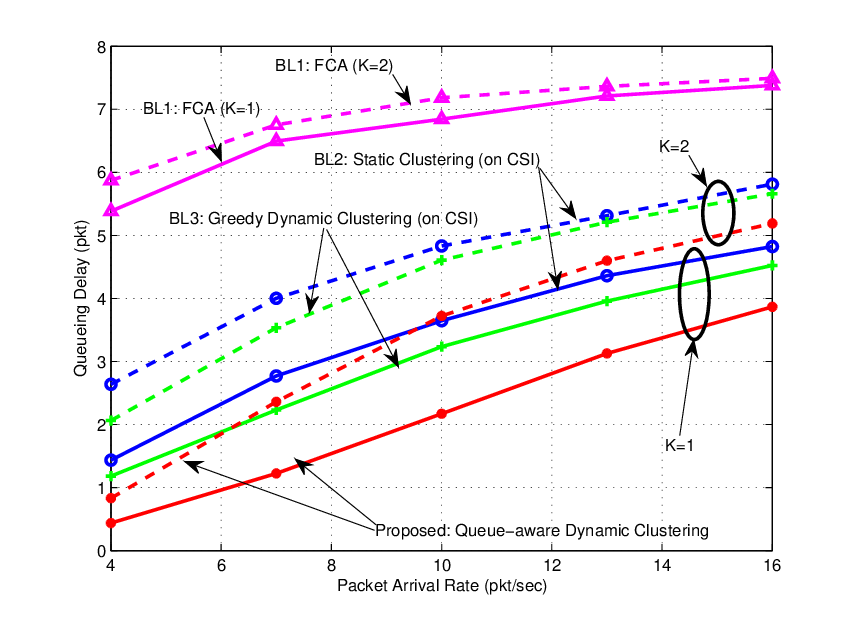
In this section, we shall compare the proposed two-timescale delay-optimal dynamic clustering and power allocation design with three baselines. Baseline 1 refers to the Fixed Channel Assignment (FCA) without cooperation among BSs in standard cellular systems with frequency reuse factor (FRF) 7. Baseline 2 and Baseline 3 refer to static clustering and greedy dynamic clustering [1, 2, 3, 4]. For any given clustering pattern, optimal power allocation is performed at each BS (Baseline 1) or CM (Baseline 2 and Baseline 3) based on available instantaneous CSI to maximize sum throughput of the cluster. In the simulation, we consider a cellular system with 19 BSs, each has a coverage of 500m. We apply the Urban Macrocell Model in 3GPP with path loss model given by P​L=34.5+35​log10⁡(r)PL=34.5+35\log_{10}(r), where rr (in m) is the distance from the transmitter to the receiver. Each element of the small scale fading channel matrix is 𝒞​𝒩​(0,1)\mathcal{CN}(0,1) distributed. The total BW is 10MHz. We consider Poisson arrival with average arrival rate λb,k\lambda_{b,k} (pck/slot). The scheduling slot duration τ\tau is 5ms. The maximum buffer size NQN_{Q} is 9 and the mean packet size N¯b,k=264\overline{N}_{b,k}=264 Kbyte.

Fig. 5 (a) illustrates the average delay per user versus transmit power with Nt=4N_{t}=4 and Nt=2N_{t}=2 and the maximum cluster size NB=3N_{B}=3. The average delay of all the schemes decreases as the transmit power or the number transmit antenna increases. Observe that the performance of Baseline 1 is inferior to that of Baseline 2 and 3, and this illustrates the gain behind base station cooperations in network MIMO systems. Furthermore, Baseline 3 outperforms Baseline 2, illustrating the benefit of dynamic clustering in network MIMO. Finally, there is significant performance gain of the proposed scheme compared to all baselines. This gain is contributed by the QSI-aware dynamic clustering as well as the QSIWFA for power control. Fig. 5 (b) illustrates the average delay versus average transmit power under different maximum cluster size NB=3N_{B}=3 and NB=2N_{B}=2. Similar observations about the performance gain could be made. Table II illustrates the complexity in terms of the CPU time of the baselines and the proposed scheme. It can be seen that the the proposed scheme can achieve significant performance gain with reasonable complexity compared with the complexity of the baselines.

Fig. 6 illustrates the average delay versus per user loading (average arrival rate λb,k\lambda_{b,k}) at transmit power of P¯b=30\overline{P}_{b}=30 dbm and number of MS per BS K=1,2K=1,2. The proposed scheme achieved significant gain over all the baselines across a wide range of input loading.

Fig. 7 illustrates the convergence property of the proposed online learning algorithm for estimating the Compact Per-cluster Per-user Potential Functions {V~n,(b,k)t}\{\widetilde{V}^{t}_{n,(b,k)}\}. We plot the transient of potential function versus slot index at a transmit power P¯b=30\overline{P}_{b}=30 dbm. It can be observed that the proposed distributive learning algorithm converges quite fast. The average delay corresponding to the the 500-th scheduling slot is 2.4069 pck, which is quite close to the optimal delay and is much smaller than the other baselines.

VII Summary

In this paper, we propose a two-timescale delay-optimal dynamic clustering and power allocation design for the downlink network MIMO systems. We show that the delay-optimal control can be formulated as an infinite-horizon average cost CPOMDP and derive an equivalent Bellman equation to solve the CPOMDP. To address the distributive requirement and the issue of exponential memory requirement and computational complexity, we propose a novel distributive online learning algorithm performed to estimate the distributive potential functions as well as the LMs. We also show that the proposed distributive online learning algorithm converges almost surely (with probability 1). We formulate the instantaneous power allocation as a Per-stage QSI-aware Interference Game played among all the CMs and propose a QSI-aware Simultaneous Iterative Water-filling Algorithm (QSIWFA) to achieve the NE. The proposed algorithm achieves significant performance gains over all the baselines due to the QSI-aware dynamic clustering and QSIWFA power control.

Appendix A: Proof of Lemma 1

Given any stationary pattern selection policy Ωc\Omega_{c}, by standard MDP techniques, the optimal power allocation policy Ωp​(𝐇,𝐐)\Omega_{p}(\mathbf{H},\mathbf{Q}) can be obtained by solving the following Bellman equation:

θΩc+VΩc​(𝐇,𝐐)\displaystyle\theta_{\Omega_{c}}+V_{\Omega_{c}}(\mathbf{H},\mathbf{Q}) =minΩp​(𝐇,𝐐){g(γ,𝐇,𝐐,Ωc,Ωp)+∑𝐇′,𝐐′Pr[𝐇′,𝐐′|𝐇′,𝐐′,Ωc,Ωp]VΩc(𝐇′,𝐐′)}\displaystyle=\min_{\Omega_{p}(\mathbf{H},\mathbf{Q})}\{g(\gamma,\mathbf{H},\mathbf{Q},\Omega_{c},\Omega_{p})+\sum_{\mathbf{H}^{\prime},\mathbf{Q}^{\prime}}\Pr[\mathbf{H}^{\prime},\mathbf{Q}^{\prime}|\mathbf{H}^{\prime},\mathbf{Q}^{\prime},\Omega_{c},\Omega_{p}]V_{\Omega_{c}}(\mathbf{H}^{\prime},\mathbf{Q}^{\prime})\}
=(a)minΩp​(𝐇,𝐐){g(γ,𝐇,𝐐,Ωc,Ωp)+∑𝐐′Pr[𝐐′|𝐇,𝐐,Ωc,Ωp]∑𝐇′Pr[𝐇′]VΩc(𝐇′,𝐐′)}\displaystyle\stackrel{{\scriptstyle(a)}}{{=}}\min_{\Omega_{p}(\mathbf{H},\mathbf{Q})}\{g(\gamma,\mathbf{H},\mathbf{Q},\Omega_{c},\Omega_{p})+\sum_{\mathbf{Q}^{\prime}}\Pr[\mathbf{Q}^{\prime}|\mathbf{H},\mathbf{Q},\Omega_{c},\Omega_{p}]\sum_{\mathbf{H}^{\prime}}\Pr[\mathbf{H}^{\prime}]V_{\Omega_{c}}(\mathbf{H}^{\prime},\mathbf{Q}^{\prime})\}
⇒(b)𝔼⁡[θ+V⁡(𝐇,𝐐)|𝐐]\displaystyle\stackrel{{\scriptstyle(b)}}{{\Rightarrow}}\mathbb{E}[\theta+V(\mathbf{H},\mathbf{Q})|\mathbf{Q}] =𝔼[minΩp​(𝐇,𝐐){g(γ,𝐇,𝐐,Ωc,Ωp)+∑𝐐′Pr[𝐐′|𝐇,𝐐,Ωc,Ωp]∑𝐇′Pr[𝐇′]V(𝐇′,𝐐′)|𝐐],∀𝐐\displaystyle=\mathbb{E}\Big[\min_{\Omega_{p}(\mathbf{H},\mathbf{Q})}\{g(\gamma,\mathbf{H},\mathbf{Q},\Omega_{c},\Omega_{p})+\sum_{\mathbf{Q}^{\prime}}\Pr[\mathbf{Q}^{\prime}|\mathbf{H},\mathbf{Q},\Omega_{c},\Omega_{p}]\sum_{\mathbf{H}^{\prime}}\Pr[\mathbf{H}^{\prime}]V(\mathbf{H}^{\prime},\mathbf{Q}^{\prime})\Big|\mathbf{Q}\Big],\forall\mathbf{Q}

where {VΩc​(𝐇,𝐐)}\{V_{\Omega_{c}}(\mathbf{H},\mathbf{Q})\} are the associated potential functions, (a) is due to (6) and (b) is obtained by taking conditional expectation (average over 𝐇\mathbf{H} conditioned on 𝐐\mathbf{Q}) on both sides, due to the i.i.d. assumption on GCSI 𝐇\mathbf{H} in Assumption 1. The optimal Ωc\Omega_{c} can be obtained by solving the following Bellman equation:

𝔼[θ+V(𝐇,𝐐)|𝐐]=minΩc​(𝐐)𝔼[minΩp​(𝐇,𝐐){g(γ,𝐇,𝐐,Ωc,Ωp)+∑𝐐′Pr[𝐐′|𝐇,𝐐,Ωc,Ωp]∑𝐇′Pr[𝐇′]V(𝐇′,𝐐′)|𝐐],∀𝐐\displaystyle\mathbb{E}[\theta+V(\mathbf{H},\mathbf{Q})|\mathbf{Q}]=\min_{\Omega_{c}(\mathbf{Q})}\mathbb{E}\Big[\min_{\Omega_{p}(\mathbf{H},\mathbf{Q})}\{g(\gamma,\mathbf{H},\mathbf{Q},\Omega_{c},\Omega_{p})+\sum_{\mathbf{Q}^{\prime}}\Pr[\mathbf{Q}^{\prime}|\mathbf{H},\mathbf{Q},\Omega_{c},\Omega_{p}]\sum_{\mathbf{H}^{\prime}}\Pr[\mathbf{H}^{\prime}]V(\mathbf{H}^{\prime},\mathbf{Q}^{\prime})\Big|\mathbf{Q}\Big],\forall\mathbf{Q}

where {V⁡(𝐇,𝐐)}\{V(\mathbf{H},\mathbf{Q})\} are the associated potential functions. Define V¯​(𝐐)=𝔼​[V​(𝐇,𝐐)|𝐐]\overline{V}(\mathbf{Q})=\mathbb{E}[V(\mathbf{H},\mathbf{Q})|\mathbf{Q}], we can obtain the equivalent Bellman equation:

θ+V¯​(𝐐)\displaystyle\theta+\overline{V}(\mathbf{Q}) =minΩc​(𝐐)𝔼[minΩp​(𝐇,𝐐){g(γ,𝐇,𝐐,Ωc,Ωp)+∑𝐐′Pr[𝐐′|𝐇,𝐐,Ωc,Ωp]V¯(𝐐′)|𝐐]\displaystyle=\min_{\Omega_{c}(\mathbf{Q})}\mathbb{E}\Big[\min_{\Omega_{p}(\mathbf{H},\mathbf{Q})}\{g(\gamma,\mathbf{H},\mathbf{Q},\Omega_{c},\Omega_{p})+\sum_{\mathbf{Q}^{\prime}}\Pr[\mathbf{Q}^{\prime}|\mathbf{H},\mathbf{Q},\Omega_{c},\Omega_{p}]\overline{V}(\mathbf{Q}^{\prime})\Big|\mathbf{Q}\Big]
=(c)minΩc​(𝐐),Ωp​(𝐐){g¯(γ,𝐐,Ωc,Ωp)+∑𝐐′Pr[𝐐′|𝐐,Ωc,Ωp]V¯(𝐐′)},∀𝐐\displaystyle\stackrel{{\scriptstyle(c)}}{{=}}\min_{\Omega_{c}(\mathbf{Q}),\Omega_{p}(\mathbf{Q})}\{\overline{g}(\gamma,\mathbf{Q},\Omega_{c},\Omega_{p})+\sum_{\mathbf{Q}^{\prime}}\Pr[\mathbf{Q}^{\prime}|\mathbf{Q},\Omega_{c},\Omega_{p}]\overline{V}(\mathbf{Q}^{\prime})\},\ \ \forall\mathbf{Q} (41)

where (c) is due to the definition of “conditional action sets” in Definition 2. Let Ω∗=(Ωc∗,Ωp∗)\Omega^{*}=(\Omega_{c}^{*},\Omega_{p}^{*}) denote the optimal control policy minimizing R.H.S. of (41) at any state 𝐐\mathbf{Q}, and θ=Lβ∗​(𝜸)=infΩLβ​(Ω,𝜸)\theta=L_{\beta}^{*}(\boldsymbol{\gamma})=\inf_{\Omega}L_{\beta}(\Omega,\boldsymbol{\gamma}) is the optimal average cost per stage. By Definition 2, we have the associated original control policy Ω∗​(𝝌)=(Ωc∗​(𝐐),Ωp∗​(𝝌))\Omega^{*}(\boldsymbol{\chi})=(\Omega_{c}^{*}(\mathbf{Q}),\Omega_{p}^{*}(\boldsymbol{\chi})), which solves Problem 1 and hence, θ\theta is also the optimal average cost per stage of Problem 1. Due to the discrete nature of pattern selection, we introduce the Pattern Selection Q-factor ℚ⁡(𝐐,C)\mathbb{Q}(\mathbf{Q},C) (∀C∈𝒞,∀𝐐\forall C\in\mathcal{C},\forall\mathbf{Q}) to facilitate the pattern selection, which is defined as

ℚ⁡(𝐐,C)≜\displaystyle\mathbb{Q}(\mathbf{Q},C)\triangleq minΩp​(𝐐){g¯(𝜸,𝐐,C,Ωp(𝐐))+∑𝐐′Pr[𝐐′|𝐐,C,Ωp(𝐐)]V¯(𝐐′)}−θ\displaystyle\min_{\Omega_{p}(\mathbf{Q})}\Big\{\overline{g}\big(\boldsymbol{\gamma},\mathbf{Q},C,\Omega_{p}(\mathbf{Q})\big)+\sum_{\mathbf{Q}^{\prime}}\Pr[\mathbf{Q}^{\prime}|\mathbf{Q},C,\Omega_{p}(\mathbf{Q})]\overline{V}(\mathbf{Q}^{\prime})\Big\}-\theta (42)
=(d)\displaystyle\stackrel{{\scriptstyle(d)}}{{=}} 𝔼[AminΩp​(𝐇,𝐐){g(𝜸,(𝐇,𝐐),C,Ωp(𝐇,𝐐))+∑𝐐′Pr[𝐐′|(𝐇,𝐐),C,Ωp(𝐇,𝐐)]V¯(𝐐′)}|𝐐]−θ\displaystyle\mathbb{E}\Big[A\min_{\Omega_{p}(\mathbf{H},\mathbf{Q})}\big\{g\big(\boldsymbol{\gamma},(\mathbf{H},\mathbf{Q}),C,\Omega_{p}(\mathbf{H},\mathbf{Q})\big)+\sum_{\mathbf{Q}^{\prime}}\Pr[\mathbf{Q}^{\prime}|(\mathbf{H},\mathbf{Q}),C,\Omega_{p}(\mathbf{H},\mathbf{Q})]\overline{V}(\mathbf{Q}^{\prime})\big\}\Big|\mathbf{Q}\Big]-\theta
=\displaystyle= R.H.S. of (11)

where (d) is due to Definition 2. Therefore, V¯​(𝐐)=minC⁡ℚ⁡(𝐐,C)\overline{V}(\mathbf{Q})=\min_{C}\mathbb{Q}(\mathbf{Q},C), Ωc∗​(𝐐)=arg⁡minC⁡ℚ⁡(𝐐,C)\Omega_{c}^{*}(\mathbf{Q})=\arg\min_{C}\mathbb{Q}(\mathbf{Q},C) and {ℚ⁡(𝐐,C)}\{\mathbb{Q}(\mathbf{Q},C)\} satisfies (11).

Appendix B: Proof of Lemma 2

Since the per-cluster potential function {V¯nt​(𝐐n)}\{\overline{V}_{n}^{t}(\mathbf{Q}_{n})\} of each queue state 𝐐n\mathbf{Q}_{n} is updated comparably often [Borkarasynchronous:1998], the only difference between the synchronous and asynchronous update is that the resultant ODE of the asynchronous update is a time-scaled version of the synchronous update [Borkarasynchronous:1998], which does not affect the convergence behavior. Therefore, we consider the convergence of related synchronous version in the following. In the following proof, we shall use ii (1≤i≤IQn1\leq i\leq I_{Q_{n}}) instead of 𝐐ni\mathbf{Q}_{n}^{i} for simplicity. since 𝜸n\boldsymbol{\gamma}_{n} is quasi-static over the timescale I, we shall omit 𝜸n\boldsymbol{\gamma}_{n} in the arguments of the function 𝐓n​(⋅)\mathbf{T}_{n}(\cdot).

We shall first show the convergence of the martingale noise in (17). Let 𝔼t\mathbb{E}_{t} and Prt\Pr_{t} denote the expectation and probability conditioned on the σ\sigma-algebra ℱt\mathcal{F}_{t}, generated by {𝐕¯n0,𝐘nk,k≤t}\{\overline{\mathbf{V}}_{n}^{0},\mathbf{Y}_{n}^{k},k\leq t\}. Define OPENSnt​(i)≜𝔼t​(Ynt​(i))=Tn,i​(𝐕¯nt)−V¯t​(i)−Tn,I​(𝐕¯nt)−V¯nt​(I))S_{n}^{t}(i)\triangleq\mathbb{E}_{t}(Y_{n}^{t}(i))=T_{n,i}(\mathbf{\overline{V}}_{n}^{t})-{\overline{V}}^{t}(i)-T_{n,I}(\mathbf{\overline{V}}_{n}^{t})-{\overline{V}_{n}}^{t}(I)), where Ynt​(i)Y_{n}^{t}(i) is the noise corrupted observation of Snt​(i)S_{n}^{t}(i) given in (17). Define δ​Mt​(i)=Ynt​(i)−𝔼t​[Ynt​(i)]\delta M^{t}(i)=Y_{n}^{t}(i)-\mathbb{E}_{t}[Y_{n}^{t}(i)], which is the martingale difference noise with property that 𝔼t​[δ​Mnt​(i)]=0\mathbb{E}_{t}[\delta M_{n}^{t}(i)]=0 and 𝔼⁡[δ​Mnt​(i)​δ​Mnt′​(i)]=0,∀t≠t′\mathbb{E}[\delta M_{n}^{t}(i)\delta M_{n}^{t^{\prime}}(i)]=0,\forall t\neq t^{\prime}. For some kk, define Mnt​(i)=∑l=ktϵlv​δ​Mnl​(i)M_{n}^{t}(i)=\sum_{l=k}^{t}\epsilon^{v}_{l}\delta M_{n}^{l}(i). Thus, from (39), we have

V¯nt+1​(i)=V¯nt​(i)+ϵtv​[St​(i)+δ​Mnt​(i)]=V¯nk​(i)+∑l=ktϵlv​Sl​(i)+Mnt​(i)\displaystyle\overline{V}_{n}^{t+1}(i)=\overline{V}_{n}^{t}(i)+\epsilon^{v}_{t}[S^{t}(i)+\delta M_{n}^{t}(i)]=\overline{V}_{n}^{k}(i)+\sum_{l=k}^{t}\epsilon^{v}_{l}S^{l}(i)+M_{n}^{t}(i) (43)

Since 𝔼t​[Mnt​(i)]=Mnt−1​(i)\mathbb{E}_{t}[M_{n}^{t}(i)]=M_{n}^{t-1}(i), {Mnt​(i)}\{M_{n}^{t}(i)\} is a martingale sequence. By Kolmogorov’s inequality, we have Prk{supk≤l≤t|Mnl(i)|≥λ}≤𝔼k​[|δ​Mnt​(i)|2]λ2≤δ​Mn¯\Pr_{k}\{\sup_{k\leq l\leq t}|M_{n}^{l}(i)|\geq\lambda\}\leq\frac{\mathbb{E}_{k}[|\delta M_{n}^{t}(i)|^{2}]}{\lambda^{2}}\leq\overline{\delta M_{n}}. By the boundedness assumption of δ​Mnt​(i)​(∀t,i)\delta M_{n}^{t}(i)\ (\forall t,i) and the property of the martingale difference noise as well as the condition on the stepsize sequence in (19), we have 𝔼k​[|Mnt​(i)|2]=𝔼k​[|∑l=ktϵlv​δ​Mnl​(i)|2]=∑l=kt𝔼k​[(ϵlv)2​(δ​Mnl​(i))2]≤δ​M¯n​∑l=kt(ϵlv)2⇒limk→∞P​rk​supk≤l≤t|Mnl​(i)|≥λ=0\mathbb{E}_{k}[|M_{n}^{t}(i)|^{2}]=\mathbb{E}_{k}[|\sum_{l=k}^{t}\epsilon^{v}_{l}\delta M_{n}^{l}(i)|^{2}]=\sum_{l=k}^{t}\mathbb{E}_{k}[(\epsilon^{v}_{l})^{2}(\delta M_{n}^{l}(i))^{2}]\leq\delta\overline{M}_{n}\sum_{l=k}^{t}(\epsilon^{v}_{l})^{2}\Rightarrow\lim_{k\to\infty}Pr_{k}{\sup_{k\leq l\leq t}|M_{n}^{l}(i)|\geq\lambda}=0. Thus, as k→∞k\to\infty, (43) goes to V¯nt+1​(i)=V¯nk​(i)+∑l=ktϵlv​Snl​(i)\overline{V}_{n}^{t+1}(i)=\overline{V}_{n}^{k}(i)+\sum_{l=k}^{t}\epsilon^{v}_{l}S_{n}^{l}(i) with probability 1. The vector form of update is given by:

𝐕¯nt+1=𝐕¯nk+∑l=ktϵlv​[𝐓⁡(𝐕¯nl)−𝐕¯nl−(Tn,I​(𝐕¯nl)−V¯nl​(I))​𝐞]\displaystyle\mathbf{\overline{V}}_{n}^{t+1}=\mathbf{\overline{V}}_{n}^{k}+\sum_{l=k}^{t}\epsilon^{v}_{l}\big[\mathbf{T}(\mathbf{\overline{V}}_{n}^{l})-\mathbf{\overline{V}}_{n}^{l}-(T_{n,I}(\mathbf{\overline{V}}_{n}^{l})-{\overline{V}}_{n}^{l}(I))\mathbf{e}\big] (44)

Next, we shall show the convergence of (44) after the Martingale noise are averaged out. Let Ωt∗\Omega_{t}^{*} denote the optimal control action attaining the minimum in 𝐓n​(𝐕nt)\mathbf{T}_{n}(\mathbf{V}_{n}^{t}). Let 𝐠¯nt\mathbf{\overline{g}}_{n}^{t} and 𝐏nt\mathbf{P}_{n}^{t} denote the conditional per-stage reward vector and conditional average transition probability matrix under Ωt∗\Omega_{t}^{*}. Denote wt=Tn,I​(𝐕¯nt)−V¯nt​(I)w^{t}=T_{n,I}(\mathbf{\overline{V}}_{n}^{t})-{\overline{V}}_{n}^{t}(I), we have

Snt\displaystyle S_{n}^{t} =𝐠¯nt+𝐏nt​𝐕¯nt−𝐕¯nt−wt​𝐞≤𝐠¯nt−1+𝐏nt−1​𝐕¯nt−𝐕¯nt−wt​𝐞\displaystyle=\mathbf{\overline{g}}_{n}^{t}+\mathbf{P}_{n}^{t}\mathbf{\overline{V}}_{n}^{t}-\mathbf{\overline{V}}_{n}^{t}-w^{t}\mathbf{e}\leq\mathbf{\overline{g}}_{n}^{t-1}+\mathbf{P}_{n}^{t-1}\mathbf{\overline{V}}_{n}^{t}-\mathbf{\overline{V}}_{n}^{t}-w^{t}\mathbf{e}
Snt−1\displaystyle S_{n}^{t-1} =𝐠¯nt−1+𝐏nt−1​𝐕¯nt−1−𝐕¯nt−1−wt−1​𝐞≤𝐠¯Ωt+𝐏nt​𝐕¯nt−1−𝐕¯nt−1−wt−1​𝐞\displaystyle=\mathbf{\overline{g}}_{n}^{t-1}+\mathbf{P}_{n}^{t-1}\mathbf{\overline{V}}_{n}^{t-1}-\mathbf{\overline{V}}_{n}^{t-1}-w^{t-1}\mathbf{e}\leq\mathbf{\overline{g}}_{\Omega_{t}}+\mathbf{P}_{n}^{t}\mathbf{\overline{V}}_{n}^{t-1}-\mathbf{\overline{V}}_{n}^{t-1}-w^{t-1}\mathbf{e}
⇒by iterating\displaystyle\stackrel{{\scriptstyle\text{by iterating}}}{{\Rightarrow}} 𝐀nt−1⋯𝐀nt−mSnt−m−C1(wt−wt−m)𝐞≤Snt≤𝐁nt−1⋯𝐁nt−mSnt−m−C1(wt−wt−m)𝐞\displaystyle\mathbf{A}_{n}^{t-1}\cdots\mathbf{A}_{n}^{t-m}S_{n}^{t-m}-C_{1}(w^{t}-w^{t-m})\mathbf{e}\leq S_{n}^{t}\leq\mathbf{B}_{n}^{t-1}\cdots\mathbf{B}_{n}^{t-m}S_{n}^{t-m}-C_{1}(w^{t}-w^{t-m})\mathbf{e}

where C1C_{1} is some constant. Since Snt​(I)=0,∀tS_{n}^{t}(I)=0,\forall t, by the assumption in (21), we have

(1−δ)​mini′​Snt−m​(i′)−C1​(wt−wt−m)≤Snt​(i)≤(1−δ)​maxi′​Snt−m​(i′)−C1​(wt−wt−m)​∀i\displaystyle(1-\delta)\min_{i^{\prime}}S_{n}^{t-m}(i^{\prime})-C_{1}(w^{t}-w^{t-m})\leq S_{n}^{t}(i)\leq(1-\delta)\max_{i^{\prime}}S_{n}^{t-m}(i^{\prime})-C_{1}(w^{t}-w^{t-m})\ \forall i
⇒{mini′⁡Snt​(i′)≥(1−δ)​mini′​Snt−m​(i′)−C1​(wt−wt−m)maxi′⁡Snt​(i′)≤(1−δ)​maxi′​Snt−m​(i′)−C1​(wt−wt−m)\displaystyle\Rightarrow\left\{\begin{array}[]{ll}\min_{i^{\prime}}S_{n}^{t}(i^{\prime})\geq(1-\delta)\min_{i^{\prime}}S_{n}^{t-m}(i^{\prime})-C_{1}(w^{t}-w^{t-m})\\ \max_{i^{\prime}}S_{n}^{t}(i^{\prime})\leq(1-\delta)\max_{i^{\prime}}S_{n}^{t-m}(i^{\prime})-C_{1}(w^{t}-w^{t-m})\end{array}\right.

Therefore maxi′⁡Snt​(i′)−mini′⁡Snt​(i′)≤(1−δ)​(maxi′⁡Snt−m​(i′)−mini′⁡Snt−m​(i′))⇒maxi′⁡Snt​(i′)−mini′⁡Snt​(i′)≤ϕk​∏l=1⌊t−km⌋(1−δk+l​m)\max_{i^{\prime}}S_{n}^{t}(i^{\prime})-\min_{i^{\prime}}S_{n}^{t}(i^{\prime})\leq(1-\delta)\big(\max_{i^{\prime}}S_{n}^{t-m}(i^{\prime})-\min_{i^{\prime}}S_{n}^{t-m}(i^{\prime})\big)\Rightarrow\max_{i^{\prime}}S_{n}^{t}(i^{\prime})-\min_{i^{\prime}}S_{n}^{t}(i^{\prime})\leq\phi_{k}\prod_{l=1}^{\lfloor\frac{t-k}{m}\rfloor}(1-\delta_{k+lm}), where ϕk>0\phi_{k}>0. Since Snt​(I)=0S_{n}^{t}(I)=0, we have maxi′⁡Snt​(i′)≥0\max_{i^{\prime}}S_{n}^{t}(i^{\prime})\geq 0 and mini′⁡Snt​(i′)≤0\min_{i^{\prime}}S_{n}^{t}(i^{\prime})\leq 0. Thus, ∀i\forall i, we have |Snt​(i)|≤maxi′⁡Snt​(i′)−mini′⁡Snt​(i′)≤ϕk​∏l=1⌊t−km⌋(1−δk+l​m)|S_{n}^{t}(i)|\leq\max_{i^{\prime}}S_{n}^{t}(i^{\prime})-\min_{i^{\prime}}S_{n}^{t}(i^{\prime})\leq\phi_{k}\prod_{l=1}^{\lfloor\frac{t-k}{m}\rfloor}(1-\delta_{k+lm}). Therefore, as t→∞t\to\infty, Snt→0S_{n}^{t}\to 0, i.e. 𝐕¯n∞\mathbf{\overline{V}}_{n}^{\infty} satisfies the fixed point equation (22). 𝐕¯n∞\mathbf{\overline{V}}_{n}^{\infty} is the potential vector, which is up to an constant vector[5]. However, due to the property that Snt​(I)=0​∀t⇒V¯nt​(I)=V¯n0​(I)​∀tS_{n}^{t}(I)=0\ \forall t\Rightarrow\overline{V}_{n}^{t}(I)=\overline{V}_{n}^{0}(I)\ \forall t, we have the convergence of the potential vector 𝐕¯n∞=limt→∞𝐕¯nt\mathbf{\overline{V}}_{n}^{\infty}=\lim_{t\to\infty}\mathbf{\overline{V}}_{n}^{t}.

Appendix C: Proof of Lemma 3

Due to the two time scale separation, the primal update of the per-cluster per-user potential can be regarded as converged to V¯n∞\overline{V}_{n}^{\infty} w.r.t the LMs {γbt}\{\gamma_{b}^{t}\} at tt-th slot. [16]. Using standard stochastic approximation theorem[15], the dynamics of the LM γb\gamma_{b} for BS b⁡(∀b∈ℬ)b\ (\forall b\in\mathcal{B}) update equation in (18) can be represented by the following ODE:

γb˙​(t)=𝔼(Ωc∗​(𝜸⁡(t)),Ωp∗​(𝜸⁡(t)))​[Pb​(t)−P¯b],∀b∈ℬ\displaystyle\dot{\gamma_{b}}(t)=\mathbb{E}^{\big(\Omega_{c}^{*}(\boldsymbol{\gamma}(t)),\Omega_{p}^{*}(\boldsymbol{\gamma}(t))\big)}[P_{b}(t)-\overline{P}_{b}],\ \forall b\in\mathcal{B} (45)

where Ωc∗​(𝜸⁡(t))\Omega_{c}^{*}(\boldsymbol{\gamma}(t)) is the converged policy in (16), Ωp∗​(𝜸⁡(t))\Omega_{p}^{*}(\boldsymbol{\gamma}(t)) is the converged policy minimizing the R.H.S. of (13) for each cluster nn, and 𝔼(Ωc∗​(𝜸⁡(t)),Ωp∗​(𝜸⁡(t)))​[⋅]\mathbb{E}^{\big(\Omega_{c}^{*}(\boldsymbol{\gamma}(t)),\Omega_{p}^{*}(\boldsymbol{\gamma}(t))\big)}[\cdot] denotes the expectation w.r.t the measure induced by (Ωc∗​(𝜸⁡(t)),Ωp∗​(𝜸⁡(t)))\big(\Omega_{c}^{*}(\boldsymbol{\gamma}(t)),\Omega_{p}^{*}(\boldsymbol{\gamma}(t))\big). Define G⁡(𝜸)=𝔼(Ωc∗​(𝜸),Ωp∗​(𝜸))​[∑ωn∈Cg¯n​(𝜸n,𝐐ni,Ω𝐩n∗​(𝐐ni))]G(\boldsymbol{\gamma})=\mathbb{E}^{\big(\Omega_{c}^{*}(\boldsymbol{\gamma}),\Omega_{p}^{*}(\boldsymbol{\gamma})\big)}[\sum_{\omega_{n}\in C}\overline{g}_{n}(\boldsymbol{\gamma}_{n},\mathbf{Q}_{n}^{i},\Omega_{\mathbf{p}_{n}}^{*}(\mathbf{Q}_{n}^{i}))], where Ωp∗​(𝜸)=arg⁡minΩp​(𝜸)​𝔼(Ωc∗​(𝜸),Ωp​(𝜸))​[∑ωn∈Cg¯n​(𝜸n,𝐐ni,Ω𝐩n​(𝐐ni))]\Omega_{p}^{*}(\boldsymbol{\gamma})=\arg\min_{\Omega_{p}(\boldsymbol{\gamma})}\mathbb{E}^{\big(\Omega_{c}^{*}(\boldsymbol{\gamma}),\Omega_{p}(\boldsymbol{\gamma})\big)}[\sum_{\omega_{n}\in C}\overline{g}_{n}(\boldsymbol{\gamma}_{n},\mathbf{Q}_{n}^{i},\Omega_{\mathbf{p}_{n}}(\mathbf{Q}_{n}^{i}))]. Since clustering pattern selection policy is discrete, we have Ωc∗​(𝜸)=Ωc∗​(𝜸+𝜹γ)\Omega_{c}^{*}(\boldsymbol{\gamma})=\Omega_{c}^{*}(\boldsymbol{\gamma}+\boldsymbol{\delta}_{\gamma}). Hence, by chain rule, we have ∂G∂γb=∑b′,k∂G∂pb′,k​∂pb′,k∂γb+𝔼(Ωc∗​(𝜸),Ωp∗​(𝜸))​[Pb​(t)−P¯b]\frac{\partial G}{\partial\gamma_{b}}=\sum_{b^{\prime},k}\frac{\partial G}{\partial p_{b^{\prime},k}}\frac{\partial p_{b^{\prime},k}}{\partial\gamma_{b}}+\mathbb{E}^{\big(\Omega_{c}^{*}(\boldsymbol{\gamma}),\Omega_{p}^{*}(\boldsymbol{\gamma})\big)}[P_{b}(t)-\overline{P}_{b}]. Since Ωp∗​(𝜸)=arg⁡minΩp​(𝜸)​𝔼(Ωc∗​(𝜸),Ωp​(𝜸))​[∑ωn∈Cg¯n​(𝜸n,𝐐ni,Ω𝐩n​(𝐐ni))]\Omega_{p}^{*}(\boldsymbol{\gamma})=\arg\min_{\Omega_{p}(\boldsymbol{\gamma})}\mathbb{E}^{\big(\Omega_{c}^{*}(\boldsymbol{\gamma}),\Omega_{p}(\boldsymbol{\gamma})\big)}[\sum_{\omega_{n}\in C}\overline{g}_{n}(\boldsymbol{\gamma}_{n},\mathbf{Q}_{n}^{i},\Omega_{\mathbf{p}_{n}}(\mathbf{Q}_{n}^{i}))], we have ∂G∂γb=0+𝔼(Ωc∗​(𝜸),Ωp∗​(𝜸))​[Pb−P¯b]=γb˙​(t)\frac{\partial G}{\partial\gamma_{b}}=0+\mathbb{E}^{\big(\Omega_{c}^{*}(\boldsymbol{\gamma}),\Omega_{p}^{*}(\boldsymbol{\gamma})\big)}[P_{b}-\overline{P}_{b}]=\dot{\gamma_{b}}(t). Therefore, we show that the ODE in (45) can be expressed as 𝜸˙​(t)=▽​G​(𝜸​(t))\dot{\boldsymbol{\gamma}}(t)=\triangledown G(\boldsymbol{\gamma}(t)). As a result, the ODE in (45) will converge to ▽​G​(𝜸)=0\triangledown G(\boldsymbol{\gamma})=0, which corresponds to the per-BS average power constraints in (5).

Appendix D: Proof of Lemma 4

Substitute the transition probability in (V-A) into (13) and then apply standard optimization techniques to minimize the R.H.S. of (13), we can obtain the closed-form optimal power control policy for given CQSI and CCSI: pb,k​(𝐇n,𝐐n)=(τN¯b,k​Δb,k​V¯n​(𝐐n)∑b′∈ωnγb′∥𝐰(b,k),b′∥2−(1+I^n,(b,k)))+p_{b,k}(\mathbf{H}_{n},\mathbf{Q}_{n})=\Big(\frac{\frac{\tau}{\overline{N}_{b,k}}\Delta_{b,k}\overline{V}_{n}(\mathbf{Q}_{n})}{\sum_{b^{\prime}\in\omega_{n}}\gamma^{b^{\prime}}\parallel\mathbf{w}_{(b,k),b^{\prime}}\parallel^{2}}-(1+\hat{I}_{n,(b,k)})\Big)^{+}, where Δb,k​V¯n​(𝐐n)=V¯n​(𝐐n)−V¯n​([𝐐n−𝐞b,k]+)\Delta_{b,k}\overline{V}_{n}(\mathbf{Q}_{n})=\overline{V}_{n}(\mathbf{Q}_{n})-\overline{V}_{n}([\mathbf{Q}_{n}-\mathbf{e}_{b,k}]^{+}). Similarly, substitute the transition probability in (28) into (27) and then apply standard optimization techniques to minimize the R.H.S. of (13), we can obtain the closed-form optimal power control policy for given LQSI and CCSI: pb,k​(𝐇n,Q)=(τN¯b,k​Δ​V¯n,(b,k)​(Q)∑b′∈ωnγb′∥𝐰(b,k),b′∥2−(1+I^n,(b,k)))+p_{b,k}(\mathbf{H}_{n},Q)=\Big(\frac{\frac{\tau}{\overline{N}_{b,k}}\Delta\overline{V}_{n,(b,k)}(Q)}{\sum_{b^{\prime}\in\omega_{n}}\gamma^{b^{\prime}}\parallel\mathbf{w}_{(b,k),b^{\prime}}\parallel^{2}}-(1+\hat{I}_{n,(b,k)})\Big)^{+}, where Δ​V¯n,(b,k)​(Q)=V¯n,(b,k)​(Q)−V¯n,(b,k)​([Q−1]+)\Delta\overline{V}_{n,(b,k)}(Q)=\overline{V}_{n,(b,k)}(Q)-\overline{V}_{n,(b,k)}([Q-1]^{+}).

Solution of Bellman equation in (13) can be obtained by offline relative value iteration[5]. Without loss of generality, we set 𝐐nI=𝟎\mathbf{Q}_{n}^{I}=\mathbf{0} as the reference state. Hence, we have normalizing equation V¯nl​(𝐐nI)=0,∀l\overline{V}_{n}^{l}(\mathbf{Q}_{n}^{I})=0,\forall l. Assume V¯nl​(𝐐n)=∑b∈ωn∑k∈𝒦V¯n,(b,k)l​(Qb,k),∀l\overline{V}_{n}^{l}(\mathbf{Q}_{n})=\sum_{b\in\omega_{n}}\sum_{k\in\mathcal{K}}\overline{V}_{n,(b,k)}^{l}(Q_{b,k}),\forall l.

At the (l−1)(l-1)-th iteration, updating policy by minimizing the R.H.S of (13) is given by p^b,kl​(𝐇n,Qb,k)=(τN¯b,k​Δ​V¯n,(b,k)l−1​(Qb,k)∑b′∈ωnγb′∥𝐰(b,k),b′∥2−1)+\hat{p}_{b,k}^{l}(\mathbf{H}_{n},Q_{b,k})=\Big(\frac{\frac{\tau}{\overline{N}_{b,k}}\Delta\overline{V}^{l-1}_{n,(b,k)}(Q_{b,k})}{\sum_{b^{\prime}\in\omega_{n}}\gamma_{b^{\prime}}\parallel\mathbf{w}_{(b,k),b^{\prime}}\parallel^{2}}-1\Big)^{+}⇒μ^b,kl(𝐇n,Qb,k)=𝔼[log(1+p^b,kl)|𝐇n,Qb,k]/N¯b,k\Rightarrow\hat{\mu}_{b,k}^{l}(\mathbf{H}_{n},Q_{b,k})=\mathbb{E}[\log(1+\hat{p}_{b,k}^{l})|\mathbf{H}_{n},Q_{b,k}]/\overline{N}_{b,k}, where μ^b,kl​(𝐇n,Qb,k)\hat{\mu}_{b,k}^{l}(\mathbf{H}_{n},Q_{b,k}) is the mean departure rate, and Δ​V¯n,(b,k)l​(Qb,k)=Vn,(b,k)l​(Qb,k)−Vn,(b,k)l​([Qb,k−1]+)\Delta\overline{V}^{l}_{n,(b,k)}(Q_{b,k})=V^{l}_{n,(b,k)}(Q_{b,k})-V^{l}_{n,(b,k)}([Q_{b,k}-1]^{+}) is the potential increment for the MS (b,k)(b,k)’s queue.

At the ll-th iteration, we determine the potential V¯nl​(𝐐n)\overline{V}_{n}^{l}(\mathbf{Q}_{n}) and θnl\theta_{n}^{l} by solving the normalizing equation V¯nl​(𝐐nI)=0\overline{V}_{n}^{l}(\mathbf{Q}_{n}^{I})=0 together with IQn=(NQ+1)K​|ωn|I_{Q_{n}}=(N_{Q}+1)^{K|\omega_{n}|} fixed point equations in (13), which is given by θn,(b,k)l=∑b∈ωn∑k∈𝒦θn,(b,k)l\theta_{n,(b,k)}^{l}=\sum_{b\in\omega_{n}}\sum_{k\in\mathcal{K}}{\theta_{n,(b,k)}^{l}} with

θn,(b,k)l=(g¯n,(b,k)​(𝜸n,Qb,k,p^b,kl​(Qb,k))+λb,k​τ​Δ​V¯n,(b,k)l​(min⁡{Qb,k+1,NQ})−μ^¯b,kl​(Qb,k)​τ​Δ​V¯n,(b,k)l​(Qb,k))\displaystyle{\theta_{n,(b,k)}^{l}}=\Big(\overline{g}_{n,(b,k)}(\boldsymbol{\gamma}_{n},Q_{b,k},\hat{p}_{b,k}^{l}(Q_{b,k}))+\lambda_{b,k}\tau\Delta\overline{V}^{l}_{n,(b,k)}(\min\{Q_{b,k}+1,N_{Q}\})-\overline{\hat{\mu}}_{b,k}^{l}(Q_{b,k})\tau\Delta\overline{V}^{l}_{n,(b,k)}(Q_{b,k})\Big) (46)

where g¯n,(b,k)\overline{g}_{n,(b,k)} is obtained by applying interchange order of double summation over bb and b′b^{\prime} of g¯n\overline{g}_{n} in (14) and decompose it into per-cluster per-user g¯n,(b,k)\overline{g}_{n,(b,k)}. μ^¯b,kl​(Qb,ki)=E⁡[μ^b,kl​(𝐇n,Qb,ki)|Qb,ki]\overline{\hat{\mu}}_{b,k}^{l}(Q_{b,k}^{i})=E[\hat{\mu}_{b,k}^{l}(\mathbf{H}_{n},Q_{b,k}^{i})|Q_{b,k}^{i}]. There are IQnI_{Q_{n}} joint 𝐐n=(Q(b,k))b∈ωn,k∈𝒦\mathbf{Q}_{n}=(Q_{(b,k)})_{b\in\omega_{n},k\in\mathcal{K}} states, but there are only NQ+1N_{Q}+1 states for Qb,k​∀b∈ωn,kQ_{b,k}\forall b\in\omega_{n},k. Hence, in the original IQnI_{Q_{n}} fixed-point equations (46), there are only NQ+1N_{Q}+1 independent fixed-point equations for each MS (b,k)(b,k) in (46). In addition, set V¯n,(b,k)l​(0)=0,∀b,k\overline{V}_{n,(b,k)}^{l}(0)=0,\forall b,k as the individual normalizing equation, which also satisfies V¯nl​(𝐐nI)=∑b∈ωn∑kV¯n,(b,k)l​(0)=0\overline{V}_{n}^{l}(\mathbf{Q}_{n}^{I})=\sum_{b\in\omega_{n}}\sum_{k}\overline{V}_{n,(b,k)}^{l}(0)=0. Hence, in the ll-th iteration, we can obtain {V¯n,(b,k)l​(Qb,k),θn,(b,k)l}\{\overline{V}_{n,(b,k)}^{l}(Q_{b,k}),\theta_{n,(b,k)}^{l}\} by solving each MS’s equivalent Bellman equation in (46). Accordingly, {V¯nl​(𝐐n),θnl}\{\overline{V}_{n}^{l}(\mathbf{Q}_{n}),\theta_{n}^{l}\} is the solution for the original IQnI_{Q_{n}} fixed-point equations (46), where V¯nl​(𝐐n)=∑b∈ωn∑kV¯n,(b,k)l​(Qb,k)\overline{V}_{n}^{l}(\mathbf{Q}_{n})=\sum_{b\in\omega_{n}}\sum_{k}\overline{V}_{n,(b,k)}^{l}(Q_{b,k}) and θnl=∑b∈ωn∑kθn,(b,k)l\theta_{n}^{l}=\sum_{b\in\omega_{n}}\sum_{k}\theta_{n,(b,k)}^{l}.

Continue the iteration until the optimal policy converges. We obtain {V¯n,(b,k)​(Qb,k),θn,(b,k)}\{\overline{V}_{n,(b,k)}(Q_{b,k}),\theta_{n,(b,k)}\}, and {V¯n​(𝐐n),θn}\{\overline{V}_{n}(\mathbf{Q}_{n}),\theta_{n}\} as a solution of (27) and (13), respectively.

Appendix E: Proof of Lemma 5

The inter-cell interference power In,(b,k)I_{n,(b,k)} is given as In,(b,k)=∑b′∈ωn′n′≠n∑b′′∈ωn′,k′′∈𝒦|𝐡(b,k),b′​𝐰(b′′,k′′),b′|2​pb′′,k′′I_{n,(b,k)}=\sum_{\begin{subarray}{c}b^{\prime}\in\omega_{n^{\prime}}\\ n^{\prime}\neq n\end{subarray}}\sum_{b^{\prime\prime}\in\omega_{n^{\prime}},k^{\prime\prime}\in\mathcal{K}}\big|\mathbf{h}_{(b,k),b^{\prime}}\mathbf{w}_{(b^{\prime\prime},k^{\prime\prime}),b^{\prime}}\big|^{2}p_{b^{\prime\prime},k^{\prime\prime}}. since the projection of (⋅)+(\cdot)^{+} is non-expansive [Bertsekasbookparalleldistributed:1989], for any two power allocation vector 𝐩(1),𝐩(2)∈ℝ+B​K\mathbf{p}_{(1)},\mathbf{p}_{(2)}\in\mathbb{R}_{+}^{BK},

|W​Fn,(b,k)​(𝐩(1))−W​Fn,(b,k)​(𝐩(2))|≤∑b′∈ωn′n′≠n∑b′′∈ωn′k′′∈𝒦|𝐡(b,k),b′​𝐰(b′′,k′′),b′|2⋅|pb′′,k′′​(1)−pb′′,k′′​(2)|,∀b∈ℬ,k∈𝒦\displaystyle|WF_{n,(b,k)}(\mathbf{p}_{(1)})-WF_{n,(b,k)}(\mathbf{p}_{(2)})|\leq\sum_{\begin{subarray}{c}b^{\prime}\in\omega_{n^{\prime}}\\ n^{\prime}\neq n\end{subarray}}\sum_{\begin{subarray}{c}b^{\prime\prime}\in\omega_{n^{\prime}}\\ k^{\prime\prime}\in\mathcal{K}\end{subarray}}\big|\mathbf{h}_{(b,k),b^{\prime}}\mathbf{w}_{(b^{\prime\prime},k^{\prime\prime}),b^{\prime}}\big|^{2}\cdot|p_{b^{\prime\prime},k^{\prime\prime}(1)}-p_{b^{\prime\prime},k^{\prime\prime}(2)}|,\ \forall b\in\mathcal{B},k\in\mathcal{K}

put the above inequality in vector form we have ‖𝐖𝐅⁡(𝐩(1))−𝐖𝐅⁡(𝐩(2))‖≤‖𝐒⋅(𝐩(1)−𝐩(2))‖\|\mathbf{WF}(\mathbf{p}_{(1)})-\mathbf{WF}(\mathbf{p}_{(2)})\|\leq\|\mathbf{S}\cdot(\mathbf{p}_{(1)}-\mathbf{p}_{(2)})\|, with the matrix 𝐒\mathbf{S} defined in (V-C). With the weighted maximum norm ∥⋅∥𝐮∞,vec\|\cdot\|^{\mathbf{u}}_{\infty,\text{vec}} and ∥⋅∥𝐮∞,mat\|\cdot\|^{\mathbf{u}}_{\infty,\text{mat}} defined above, ∀𝐩(1),𝐩(2)∈ℝ+B​K\forall\mathbf{p}_{(1)},\mathbf{p}_{(2)}\in\mathbb{R}_{+}^{BK} and ∀𝐮∈ℝ+B​K\forall\mathbf{u}\in\mathbb{R}_{+}^{BK} we have ‖𝐖𝐅⁡(𝐩(1))−𝐖𝐅⁡(𝐩(2))‖∞,vec𝐮≤‖𝐒⋅(𝐩(1)−𝐩(2))‖∞,vec𝐮≤‖𝐒‖∞,mat𝐮​‖(𝐩(1)−𝐩(2))‖∞,vec𝐮\|\mathbf{WF}(\mathbf{p}_{(1)})-\mathbf{WF}(\mathbf{p}_{(2)})\|^{\mathbf{u}}_{\infty,\text{vec}}\leq\|\mathbf{S}\cdot(\mathbf{p}_{(1)}-\mathbf{p}_{(2)})\|^{\mathbf{u}}_{\infty,\text{vec}}\leq\|\mathbf{S}\|^{\mathbf{u}}_{\infty,\text{mat}}\|(\mathbf{p}_{(1)}-\mathbf{p}_{(2)})\|^{\mathbf{u}}_{\infty,\text{vec}}, which is a contraction of the mapping 𝐖𝐅\mathbf{WF}, if ‖𝐒‖∞,mat𝐮<1\|\mathbf{S}\|^{\mathbf{u}}_{\infty,\text{mat}}<1 is satisfied. By the theorem on convergence of contracting iterations [Bertsekasbookparalleldistributed:1989], we can prove the existence and uniqueness of NE.

References

  • [1] F. Boccardi and H. Huang, “Limited downlink network coordination in cellular networks,” in IEEE International Symposium on Personal, Indoor and Mobile Radio Communications (PIMRC), Athens, Greece, Sep. 2007, pp. 1–5.
  • [2] J. Zhang, R. Chen, J. G. Andrews, A. Ghosh, and R. W. Heath, “Networked MIMO with clustered linear precoding,” IEEE.J.TCOM, vol. 8, no. 4, pp. 1910–1921, Apr. 2009.
  • [3] F. Boccardi, H. Huang, and A. Alexiou, “Network MIMO with reduced backhaul requirements by mac coordination,” in Asilomar Conference on Signals, Systems and Computers (ACSSC), California, USA, Oct. 2008, pp. 1125–1129.
  • [4] A. Papadogiannis, D. Gesbert, and E. Hardouin, “A dynamic clustering approach in wireless networks with multi-cell cooperative processing,” in IEEE Int. Conf. on Commun. (ICC), Beijing, China, May 2008, pp. 4033–4037.
  • [5] D. P. Bertsekas, Dynamic Programming and Optimal Control, 3rd ed. Massachusetts: Athena Scientific, 2007.
  • [6] W. B. Powell, Approximate dynamic programming: solving the curses of dimensionality, 1st ed. United Kingdom: Wiley-Interscience, 2007.
  • [7] D. P. Palomar and M. Chiang, “A tutorial on decomposition methods for network utillity maximization,” IEEE J. Sel. Areas Commun., vol. 24, no. 8, pp. 1439 – 1451, Aug. 2006.
  • [8] J. Tsitsiklis, “Np-hardness of checking the unichain condition in average cost mdps,” Operations Research Letters, vol. 35, no. 3, pp. 319–323, May 2007.
  • [9] V.S.Borkar, “An actor-critic algorithm for constrained markov decision processes,” in Systems Control Lett. 54, 2005, pp. 207–213.
  • [10] S. Boyd and L. Vandenberghe, Convex Optimization. Cambrige UK: Cambrige Univ. Press, 2004.
  • [11] Y. Cui, Q. Huang, and V. K. N. Lau, Queue-Aware Dynamic Clustering and Power Allocation for Network MIMO Systems via Distributive Stochastic Learning, full version. [Online]. Available: http://arxiv.org/abs/1006.3919
  • [12] D. Bertsekas and J. Tsitsiklis, Neuro-dynamic programming: an overview, 2002.
  • [13] X. R. Cao, Stochastic Learning and Optimization: A Sensitivity-Based Approach, 1st ed. New York: Springer, 2007.
  • [14] J. Abounadi, D. Bertsekas, and V. S. Borkar, “Learning algorithms for markov decision processes with average cost,” SIAM Journal on Control and Optimization, vol. 40, no. 3, pp. 681–698, 2001.
  • [15] V. S. Borkar, Stochastic Approximation: A Dynamical Systems Viewpoints, 1st ed. United Kingdom: Cambridge University Press, 2008, ch. 6.
  • [16] V.S.Borkar, “Stochastic approximation with two time scales,” in Systems Control Lett. 29, 1997, pp. 291–294.
  • [17] G. Scutari, D. P. Palomar, and S. Barbarossa, “Competitive design of multiuser MIMO systems based on game theory: A unified view,” IEEE J. Sel. Areas Commun., vol. 26, no. 7, Sep. 2008.
  • [18] J. N. Tsitsiklis and B. V. Roy, “Feature-based methods for large scale dynamic programming,” Machine Learning, vol. 22, Mar. 1996.
Refer to caption
Fig. 1: Motivating Example of the advantage of QSI-based Clustering versus traditional CSI-based Clustering in Network MIMO Systems. For example, CSI-based clustering will always choose Clustering Pattern 1 (Red). This will create an interference profile in favor of MS2 and MS4 regardless of the queue state in MS2 and MS4. When the queues of MS2 and MS4 are empty, Clustering Pattern 1 will no longer be a good choice. On the contrary, the QSI-based clustering method will choose between Clustering Pattern 1 (red) and Clustering Pattern 2 (Blue) based on the queue states of the mobiles. As a result, it could dynamically creates a favorable interference profile to selected mobiles based on their queue states.
Refer to caption
(a) System Model
Refer to caption
(b) Control Architecture
Fig. 2: System model and control architecture of network MIMO systems. The dotted lines and solid lines on Fig 2. (b) denote the control path and data path, respectively.
Refer to caption
Fig. 3: Algorithm Flow of the Proposed Online Distributive Primal-Dual Learning Algorithm with Per-stage QSI-aware Interference Game and Simultaneous Updates on Potential Functions and LMs.
Scheme CPU Time (s)
BL1: FCA 0.2218e-004
BL2: Static Clustering (on CSI) 1.9098e-004
BL3: Greedy Dynamic Clustering (on CSI) 0.0012
Proposed Queue-aware Dynamic Clustering 0.0094
TABLE II: Running time complexity of the baselines and the proposed scheme. The number of cells B=19B=19, the maximum cluster size NB=3N_{B}=3, the number of MSs per BS K=1K=1, the number of antenna per-BS Nt=4N_{t}=4, the average arrival rate λb,k=10\lambda_{b,k}=10 pck/slot and the resolution level d=3d=3.
Refer to caption
Fig. 4: Probability that condition ‖𝐒‖∞,mat𝐮<1\|\mathbf{S}\|^{\mathbf{u}}_{\infty,\text{mat}}<1 is satisfied versus user location. The number of cells B=19B=19, the number of MSs per cell K=1K=1, the maximum cluster size NB=3N_{B}=3, the number of transmit antennas Nt=4N_{t}=4.
Refer to caption
(a) Average delay per user versus transmit power at the number of antenna per-BS Nt=4,2N_{t}=4,2 and the maximum cluster size NB=3N_{B}=3.
Refer to caption
(b) Average delay per user versus transmit power at the maximum cluster size NB=3,4N_{B}=3,4 and the number of antenna per-BS Nt=4N_{t}=4.
Fig. 5: Average delay per user versus transmit power. The number of MSs per BS K=1K=1, the average arrival rate λb,k=10\lambda_{b,k}=10 pck/slot and the resolution level d=3d=3.
Refer to caption
Fig. 6: Average delay per user versus per-user loading (average arrival rate λb,k\lambda_{b,k}) at the number of MSs per BS K=1K=1 and K=2K=2 at the transmit power P¯b=35\bar{P}_{b}=35 dbm. The maximum cluster size NB=3N_{B}=3, the number of transmit antenna at each BS Nt=4N_{t}=4, and the resolution level d=3d=3.
Refer to caption
Fig. 7: Convergence property of the proposed distributive stochastic learning algorithm via stochastic approximation. The transmit power P¯b=35\bar{P}_{b}=35 dbm, the maximum cluster size NB=3N_{B}=3, the number of transmit antenna at each BS Nt=4N_{t}=4, the number of MSs per BS K=1K=1 and the resolution level d=3d=3. The figure illustrates instantaneous per-cluster potential function values versus instantaneous slot index. The boxes indicated the mean delay of various schemes at three selected slot indices.