Influence of vortices and phase fluctuations on thermoelectric transport properties of superconductors in a magnetic field

Andreas Andersson Email: anan02@kth.se Affiliation: Theoretical Physics, Royal Institute of Technology, AlbaNova, SE-106 91 Stockholm, Sweden Jack Lidmar Email: jlidmar@kth.se Affiliation: Theoretical Physics, Royal Institute of Technology, AlbaNova, SE-106 91 Stockholm, Sweden

August 24, 2026

Abstract

We study heat transport and thermoelectric effects in two-dimensional superconductors in a magnetic field. These are modeled as granular Josephson-junction arrays, forming either regular or random lattices. We employ two different models for the dynamics, relaxational model-A dynamics or resistively and capacitively shunted Josephson junction (RCSJ) dynamics. We derive expressions for the heat current in these models, which are then used in numerical simulations to calculate the heat conductivity and the Nernst coefficient for different temperatures and magnetic fields. At low temperatures and zero magnetic field the heat conductivity in the RCSJ model is calculated analytically from a spin wave approximation, and is seen to have an anomalous logarithmic dependence on the system size, and also to diverge in the completely overdamped limit $C\to 0$ . From our simulations we find at low magnetic fields that the Nernst signal displays a characteristic “tilted hill” profile similar to experiments and a nonmonotonic temperature dependence of the heat conductivity. We also investigate the effects of granularity and randomness, which become important for higher magnetic fields. In this regime geometric frustration strongly influences the results in both regular and random systems and leads to highly nontrivial magnetic field dependencies of the studied transport coefficients.

pacs

74.81.-g, 74.25.F-, 74.25.fg, 74.25.Uv, 74.78.-w

I Introduction

Thermoelectric effects in superconductors are of considerable interest, since they provide an important probe of fluctuations and correlations in these materials. Such effects have gained an increasing amount of attention since the recent measurements of the Nernst effect in the pseudogap phase of underdoped high- $T_{c}$ cuprates, where a remarkably large effect was observed [1, *WangOng2006]. The Nernst effect has since then been measured in many other materials, e.g., in superconducting thin films [3, *PourretBehnia_NJP2009] and in the iron-pnictides [5]. The Nernst effect is usually very small for conventional metals, making it a particularly sensitive probe of superconducting fluctuations. Theoretical and numerical studies have described the large Nernst effect either in terms of superconducting fluctuations of Gaussian nature [6, 7, 8, 9, *Michaeli2009a], or as fluctuations of the phase of the order parameter, i.e., as a result of vortices [2, 11, 12]. Other explanations of nonsuperconducting origin have also been put forward, e.g., proximity to a quantum critical point [13, *Bhaseen2009, 15], quasiparticles [16, 17], stripe order [18], etc. Here we will focus exclusively on the effects of phase fluctuations and vortices on heat and charge transport. Phase fluctuations were early on proposed to play a key role in the pseudogap phase of underdoped cuprates [19]. In quasi-two-dimensional superconducting films and Josephson-junction arrays they are known to be the dominant fluctuations [20, *Berezinskii2, *KT].

In this paper we study the heat transport and the thermoelectric response in two-dimensional granular superconductors or Josephson- junction arrays, using two widely employed models for the dynamics, (i) relaxational model-A dynamics, described by a Langevin equation, or (ii) resistively and capacitively shunted Josephson junction (RCSJ) dynamics. These are well suited for numerical simulation studies, and have been used extensively to calculate electric and magnetic static and dynamic properties, and to study vortex dynamics under influence of electric currents [23, 24, 25, 26]. The calculation of thermoelectric properties is, however, less straightforward. Previous simulation studies have used time-dependent Ginzburg-Landau theory [7], phase-only XY models [11] with Langevin dynamics, or vortex dynamics [12]. They have been limited to rather narrow parameter regimes with a focus on explaining the large Nernst effect seen in the pseudogap phase of underdoped cuprates. Here we present a comprehensive study of heat conductivity, thermoelectric effects, and resistivity for a broad range of parameters. We also investigate the effects of a granular structure. The models are defined on a discrete lattice and can be experimentally realized in granular superconductors and artificially fabricated Josephson-junction arrays. At low magnetic fields discreteness effects become less important so that our results in this regime are relevant also for homogenous bulk superconductors. On the other hand, in granular superconductors transport properties are strongly affected by discreteness and geometric frustration effects [27]. This is particularly true at high magnetic fields when the inter-vortex distance becomes comparable to the granularity. This leads to a rich structure in, e.g., the Nernst signal as the magnetic field is varied, with anomalous sign changes occurring in the vicinity of special commensurate fillings [28].

To start with, let us first recall that the heat current density ${\bf J}^{Q}$ and electric current density ${\bf J}$ are related to the thermodynamic forces, the electric field ${\bf E}$ and the temperature gradient $-\nabla T$ , by the standard phenomenological linear relations

\begin{pmatrix}{\bf J}^{Q}\\ {\bf J}\end{pmatrix}=\begin{pmatrix}\tilde{\kappa}&\tilde{\alpha}\\ \alpha&\sigma\end{pmatrix}\begin{pmatrix}-\nabla T\\ {\bf E}\end{pmatrix},

(1)

where the thermoelectric and electrothermal tensors obey the Onsager relation $\tilde{\alpha}=T\alpha$ . The Nernst coefficient $\nu$ is defined as the off-diagonal response of the electric field $E_{y}$ to an applied temperature gradient $\nabla_{x}T$ in a transverse magnetic field $B_{z}$ ,

\nu=\frac{e_{N}}{B_{z}}=\frac{1}{B_{z}}\frac{E_{y}}{(-\nabla_{x}T)},

(2)

where $e_{N}$ is the so called Nernst signal. Both the Nernst effect and the heat conductivity are measured under the condition of zero electric current, such that

	$\displaystyle e_{N}$	$\displaystyle=\frac{\alpha_{xy}\sigma_{xx}-\alpha_{xx}\sigma_{xy}}{\sigma_{xx}^{2}+\sigma_{xy}^{2}},$		(3)
	$\displaystyle\kappa$	$\displaystyle=\tilde{\kappa}-\tilde{\alpha}\sigma^{-1}\alpha.$		(4)

In a system with no Hall effect ( $\sigma_{xy}=0$ ), which is the case for the models studied below, Eq. (3) reduces to $e_{N}=\alpha_{xy}/\sigma_{xx}$ .

In a phase-fluctuating superconductor, mobile vortices, either thermally excited or induced by an applied magnetic field, may significantly affect transport properties. An applied electric current ${\bf J}$ will exert a perpendicular force on the vortices and their motion will generate a transverse electric field ${\bf E}=-{\bf v}\times{\bf B}$ parallel to ${\bf J}$ , thus causing a finite flux-flow resistivity. Vortex motion can also be caused by a temperature gradient, thereby generating an electric field perpendicular to both the magnetic field and the temperature gradient. The Nernst coefficient defined in Eq. (2) can be seen simply as the diagonal response ${\bf v}=-\nu\nabla T$ of the vortex velocity to the temperature gradient. For this reason it is plausible that a large Nernst signal is expected in the vortex liquid phase.

Via an Onsager relation a heat current can then be generated from an applied electric current. The vortices therefore also contribute to the heat conductivity, although other heat carriers, e.g., phonons or quasiparticles, probably dominate. From the vortex point of view it is natural to consider the applied current as the driving force and the electric field, which is proportional (but perpendicular) to the vortex current, as the response. This yields an alternative, but equivalent formulation of the linear relations in Eq. (1)

\begin{pmatrix}{\bf J}^{Q}\\ {\bf E}\end{pmatrix}=\begin{pmatrix}\kappa&\tilde{\beta}\\ \beta&\rho\end{pmatrix}\begin{pmatrix}-\nabla T\\ {\bf J}\end{pmatrix},

(5)

where $\beta=-\tilde{\beta}/T=-\sigma^{-1}\alpha$ . This is the approach employed in our simulations. Instead of calculating $e_{N}$ through other transport coefficients, i.e., using Eq. (3), we obtain the Nernst signal directly as $e_{N}=\beta_{yx}=\tilde{\beta}_{xy}/T$ for ${\bf J}=0$ . The longitudinal heat conductivity is just the diagonal components of the tensor $\kappa$ in Eq. (5), and $\rho=\sigma^{-1}$ is the resistivity.

The picture described above applies when the vortices are free to move in response to the driving forces. Pinning of vortices to material defects, grain boundaries, etc., can lead to dramatic changes of the transport properties.

The paper is organized as follows. In Sec. II we introduce the models and their dynamics, Langevin or RCSJ, on general two-dimensional (2D) lattices. In Sec. III we derive an expression for the heat current for the models studied. This has over the years proven to be a subtle task, especially in the presence of a magnetic field. We present two separate routes to finding the explicit form of the heat current for Langevin and RCSJ dynamics. In addition we show, using a functional integral approach, that the Nernst signal indeed can be calculated from a Kubo formula involving the heat current. Section IV discusses the thermal conductivity at zero magnetic field in the low temperature limit, where a spin wave approximation is applicable. Our analytic calculations reveal a logarithmic system size dependence of $\kappa$ in this regime for the RCSJ case. In Sec. V we give some technical details of our numerical simulations, and in the last part, Sec. VI, the results of our numerical simulations on square and irregular lattices are presented. We consider the case of zero and weak magnetic fields as well as the high field limit, where the transport coefficients are severely affected by geometric frustration. In the weak magnetic field limit the results are discussed in relation to previous theoretical works and experiments.

II Models

We model a 2D granular superconductor (of size $L\times L$ ) as an array of superconducting grains connected by Josephson junctions. These grains may or may not be ordered and connected in a regular fashion. The supercurrent flowing between two superconducting grains $i$ and $j$ is given by the Josephson current-phase relation

	$\displaystyle I_{ij}^{s}$	$\displaystyle=I^{c}_{ij}\sin\gamma_{ij},$		(6)
	$\displaystyle\gamma_{ij}$	$\displaystyle=\theta_{i}-\theta_{j}-\frac{2\pi}{\Phi_{0}}A_{ij},\qquad A_{ij}=\int_{{\bf r}_{i}}^{{\bf r}_{j}}{\bf A}\cdot d{\bf r},$		(7)

where $I_{ij}^{c}$ is the critical current of the junction, $\Phi_{0}=h/2e$ is the superconducting flux quantum, and $\theta_{i}$ is the superconducting phase of grain $i$ . The grains are assumed to be small enough ( $\lesssim$ the coherence length) that the phase is constant over each grain. Further, ${\bf A}$ is the vector potential, which we here separate into two parts

{\bf A}({\bf r},t)={\bf A}_{\text{ext}}({\bf r})+\frac{\Phi_{0}}{2\pi}\bm{\Delta}(t),

(8)

where ${\bf A}_{\text{ext}}({\bf r})$ is constant in time and corresponds to a uniform magnetic field ${\bf B}=\nabla\times{\bf A}$ perpendicular to the array, and $\bm{\Delta}(t)=(\Delta_{x}(t),\Delta_{y}(t))$ is spatially uniform, but time dependent and is necessary to include in order to describe temporal fluctuations in the average electric field $\bar{\bf E}=-\frac{\Phi_{0}}{2\pi}\dot{\bm{\Delta}}$ , when periodic boundary conditions are used [25, 26]. Local fluctuations in the magnetic field ${\bf B}$ and hence ${\bf A}$ are ignored.

II.1 Langevin dynamics

The Langevin dynamics represents a phase-only description of the time-dependent Ginzburg-Landau dynamics (TDGL) in uniform magnetic field. The phenomenological equations of motion for $\{\theta\}$ and $\bm{\Delta}$ are of local relaxation type

$\displaystyle\gamma\dot{\theta}_{i}$	$\displaystyle=-\frac{1}{\hbar}\frac{\partial H}{\partial\theta_{i}}+\eta_{i}$	(9)
$\displaystyle\gamma_{\Delta}\dot{\bm{\Delta}}$	$\displaystyle=-\frac{1}{\hbar}\frac{\partial H}{\partial\bm{\Delta}}+\bm{\zeta}$	(10)
$\displaystyle H$	$\displaystyle=-\sum_{\left<{ij}\right>}J_{ij}\cos\gamma_{ij},$	(11)

where the time constant $\gamma$ is dimensionless and $\gamma_{\Delta}=\gamma L^{2}$ , $H$ is the XY model Hamiltonian, and $\eta_{i}$ and $\bm{\zeta}$ are Gaussian stochastic white noise processes.

Refer to caption — Figure 1: Equivalent circuit model for Langevin dynamics. The cross denotes the Josephson junction with critical current $I_{ij}^{C}$ .

These equations can be cast in the form of circuit equations for an electric circuit built up using the elements displayed in Fig. 1, where each site $i$ is connected via a resistor $R_{0}=\hbar/4e^{2}\gamma$ to ground:

	$\displaystyle\gamma\dot{\theta}_{i}$	$\displaystyle=\frac{V_{i}}{2eR_{0}}=-\frac{1}{2e}\sum_{j\in\mathcal{N}_{i}}I_{ij}^{s}+\eta_{i},$		(12)
	$\displaystyle\gamma_{\Delta}\dot{\bm{\Delta}}$	$\displaystyle=\frac{1}{2e}\bigg(\sum_{\left<{ij}\right>}I_{ij}^{s}\mathbf{r_{ji}}-L^{2}\bar{\mathbf{J}}^{\text{ext}}\bigg)+\bm{\zeta}.$		(13)

The sum in the first equation is taken over the set $\mathcal{N}_{i}$ of superconducting grains connected to $i$ and is equivalent to a lattice divergence. In the second equation $\left<{ij}\right>$ denotes a sum over all links in the system. The vector $\mathbf{r}_{ji}=\mathbf{r}_{j}-\mathbf{r}_{i}$ goes from site $i$ to site $j$ and $\bar{\mathbf{J}}^{\text{ext}}$ is a fixed external current density. The Gaussian white noise terms $\eta_{i}$ and $\bm{\zeta}$ , which now can be interpreted as Johnson-Nyquist noise in the resistors $R_{0}$ , have the correlations

	$\displaystyle\left<{\eta_{i}(t)}\right>=0,$	$\displaystyle\quad\left<{\eta_{i}(t)\eta_{j}(t^{\prime})}\right>=\frac{2k_{B}T\gamma}{\hbar}\delta_{ij}\delta(t-t^{\prime}),$		(14)
	$\displaystyle\left<{\bm{\zeta}(t)}\right>=0,$	$\displaystyle\quad\left<{\zeta_{\mu}(t)\zeta_{\nu}(t^{\prime})}\right>=\frac{2k_{B}T\gamma_{\Delta}}{\hbar}\delta_{\mu\nu}\delta(t-t^{\prime}).$		(15)

II.2 RCSJ dynamics

In the RCSJ model each Josephson junction with critical current $I^{c}_{ij}$ is shunted by both a resistor $R_{ij}$ and a capacitor $C_{ij}$ , see Fig. 2. The RSJ model is obtained as a special case when setting $C_{ij}=0$ . We write the total current from site $i$ to site $j$ as a sum of the super-, resistive, capacitative, and noise currents

	$\displaystyle I_{ij}^{\text{tot}}$	$\displaystyle=I_{ij}^{s}+I_{ij}^{R}+I_{ij}^{C}+I_{ij}^{n}$
		$\displaystyle=I_{ij}^{c}\sin\gamma_{ij}+\frac{V_{ij}}{R_{ij}}+C_{ij}\dot{V}_{ij}+I_{ij}^{n},$		(16)

where the voltage between grain $i$ and $j$ is

V_{ij}\equiv V_{i}-V_{j}-\dot{A}_{ij}=\frac{\hbar}{2e}\dot{\gamma}_{ij},

(17)

and the Johnson-Nyquist noise in the resistors has zero mean $\left<{I_{ij}^{n}}\right>=0$ and covariance

\left<{I_{ij}^{n}(t)I_{kl}^{n}(t^{\prime})}\right>=\frac{2k_{B}T}{R_{ij}}(\delta_{ik}\delta_{jl}-\delta_{il}\delta_{jk})\delta(t-t^{\prime}).

(18)

The equations of motion for the phases $\{\theta_{i}\}$ and the twists $\bm{\Delta}$ are obtained from local current conservation at each grain

\displaystyle\sum_{j\in\mathcal{N}_{i}}(I_{ij}^{\text{tot}}-I_{ij}^{\text{tr}})=0.

(19)

Here we introduced a “transport current” $I_{ij}^{\text{tr}}$ , which is a static, divergence free current distribution, satisfying any external boundary conditions, but is otherwise arbitrary. One may, for instance, connect some nodes to fixed external current sources or sinks. In the present work we will usually use periodic boundary conditions instead, together with the condition of a fixed average current density $\bar{\bf J}^{\text{ext}}$ in the system,

\displaystyle\sum_{\left<{ij}\right>}I_{ij}^{\text{tot}}\mathbf{r}_{ji}

\displaystyle=\sum_{\left<{ij}\right>}I_{ij}^{\text{tr}}\mathbf{r}_{ji}=L^{2}\bar{\mathbf{J}}^{\text{ext}}.

(20)

For model purposes we may define a local current density on the links of the lattice as

\mathbf{J}(\mathbf{r})=\sum_{\left<{ij}\right>}\int_{\mathbf{r}_{i}}^{\mathbf{r}_{j}}I^{\text{tot}}_{ij}\delta(\mathbf{r}-\mathbf{r^{\prime}})d\mathbf{r^{\prime}},

(21)

which directly leads to Eq. (20) when averaged over the system.

II.3 Lattice structure

We are interested in modeling both regular and random granular superconductors. At low magnetic fields the vortex separation is large compared to the granules and the lattice structure does not matter much. In this regime the models approximate bulk superconductors. In the opposite limit of high magnetic fields the lattice structure is important as frustration effects strongly influence the transport properties. Note that the formulation of the models defined above is independent of lattice structure. We will limit ourselves to two dimensions in the present work. In our simulations presented below in Sec. VI we consider not only square lattices, but also random lattices appropriate as models of random granular superconductors. These irregular lattices are constructed by generating a set of randomly distributed points ${\bf r}_{i}=(x_{i},y_{i})$ with unit density on a square and connecting nearest neighbors by Delaunay triangulation. To control the randomness we use the parameter $d_{\text{min}}$ , which is the shortest allowed distance between any two points in the system. Large values of $d_{\text{min}}$ will thus create a relatively ordered lattice structure, whereas lattices with small $d_{\text{min}}$ values are more disordered. For example, a given value of $d_{\text{min}}=\{0.0,0.4,0.6,0.8\}$ corresponds to a distribution of grain size diameters with standard deviation $\{0.30,0.23,0.15,0.08\}$ , respectively. Examples can be seen in Fig. 15. For the random lattices we use two different models, one where the critical current of every junction is set to a constant $I^{c}_{ij}=I^{c}$ and one where the critical current is proportional to the contact length $d^{\perp}_{ij}$ between the grains, $I^{c}_{ij}\sim d^{\perp}_{ij}$ (in the RCSJ case we also take $R^{-1}_{ij}\sim d^{\perp}_{ij}$ and $C_{ij}\sim d^{\perp}_{ij}$ ). This length is simply the distance between the points in the dual Voronoi lattice, see Fig. 3.

II.4 Transport coefficients

In the models defined above the only nonzero transport coefficients are the Nernst signal $e_{N}$ , the diagonal thermal conductivity $\kappa$ and the electrical resistivity $\rho$ . These may be obtained from equilibrium correlation functions using Kubo formulas [29, 30]. While $\rho$ relates ${\bf E}$ to a mechanical perturbation, $e_{N}$ and $\kappa$ give the response to a nonmechanical property, namely a temperature gradient, and the applicability of a standard Kubo formula is not evident. Nevertheless, we show in the next section that the transport coefficients can be expressed in standard form as

$\displaystyle e_{N}$	$\displaystyle=\frac{\Omega}{k_{B}T^{2}}\int^{\infty}_{0}\big<{\bar{E}_{y}(t)\bar{J}^{Q}_{x}(0)}\big>dt,$	(22)
$\displaystyle\kappa$	$\displaystyle=\frac{\Omega}{k_{B}T^{2}}\int^{\infty}_{0}\big<{\bar{J}^{Q}_{x}(t)\bar{J}^{Q}_{x}(0)}\big>dt,$	(23)
$\displaystyle\rho$	$\displaystyle=\frac{\Omega}{k_{B}T}\int^{\infty}_{0}\big<{\bar{E}_{y}(t)\bar{E}_{y}(0)}\big>dt,$	(24)

where $\Omega=L_{x}L_{y}$ is the area of the system. In these equations $\bar{E}_{y}=-(\Phi_{0}/2\pi)\dot{\Delta}_{y}$ is the average electric field in the $y$ -direction and

\bar{J}^{Q}_{x}=\frac{1}{\Omega}\sum_{\left<{ij}\right>}\left(x_{ji}\frac{1}{2}(V_{i}+V_{j})-x_{ij}^{c}\dot{A}_{ij}\right)(I_{ij}^{\text{tot}}-I_{ij}^{\text{tr}})

(25)

is the average heat current in the $x$ -direction, with $x_{ji}=x_{j}-x_{i}$ and $x_{ij}^{c}=(x_{i}+x_{j})/2$ . This form of the heat current, which is one of our main results, will be explicitly derived in the next section for the specific models under consideration.

III Heat current

In order to calculate thermoelectric effects and the heat conductivity an expression for the heat current is needed. Several microscopic derivations of the heat current in superconductors has been given in the literature [31, 32, 33, 34]. The presence of a magnetic field yields a complication in that the total energy and charge currents consist of magnetization currents in addition to the transport currents [35, 36].

Rather than relying on these microscopic expressions we derive here, within the framework of the models defined in Sec. II, an expression for the heat current that can be used consistently in our calculations. Below we will first derive the energy current by considering the continuity equation for the energy density. This gives the heat current after subtracting the nondissipative energy transport, except for a magnetization contribution, which is calculated separately in Sec. III.1.3.

Since we are interested in the response of the system to an applied temperature gradient, which is a nonmechanical thermodynamic force, the standard derivation of a Kubo formula does not hold. One approach is to follow Luttinger [30], and introduce a “gravitational” field, which couples to the energy density, and then proceed with the calculation of the response to perturbations in that field. For the present models, however, there is an alternative route. With the dynamics governed by stochastic equations, Eqs. (12-13) or (19-20), in which the temperature enters via the strength of the stochastic noise, it is possible to introduce local temperature variations, such as a temperature gradient, and calculate the resulting response. This calculation, done in Sec. III.2 gives us both the Kubo formula Eq. (22) and the heat current Eq. (25). Note that in this setting, each point in the model, or more precisely, each resistor in the circuit, is in contact with a local heat bath. For finite gradients one cannot expect the heat current to be automatically conserved, since the resistors act as sinks and sources. For an infinitesimal thermal gradient the heat current will, however, be conserved on average. Alternatively, one could adjust the local temperatures to make sure that heat is conserved on average also for finite temperature gradients. Such self-consistent temperatures have been employed in studies of heat conductivity in harmonic lattices [37]. For the problem at hand, however, the temperature profile is determined by the total heat transport, including phonons, etc, so an externally imposed temperature gradient is probably more realistic. For the linear response the form of the profile should not matter as long as it is smooth. We will use a linear temperature profile below.

III.1 Heat current from continuity equations

In this section we will derive the heat current expressions for granular superconductors described by Langevin and RCSJ dynamics, as used in our simulations. First, however, it is useful to discuss briefly the continuum formulation. Starting from the thermodynamic relation

Tds=de-\mu dn-{\bf H}\cdot d{\bf B}-{\bf E}\cdot d{\bf D}

(26)

for a superconductor in a magnetic field ${\bf H}$ and electric field ${\bf E}$ , where $s$ and $e$ are the entropy and energy densities, $\mu$ the chemical potential, and $n$ the density of charge carriers (with charge $q$ ), one obtains for the heat current density

{\bf J}^{Q}={\bf J}_{\text{tot}}^{E}-\frac{\mu}{q}{\bf J}-{\bf E}\times{\bf H},

(27)

where ${\bf J}$ is the electric transport current density. The total energy current density is the sum of two parts, a nonmagnetic part and Poynting’s vector,

\displaystyle{\bf J}^{E}_{\text{tot}}={\bf J}^{E}+\frac{1}{\mu_{0}}{\bf E}\times{\bf B},

(28)

and the transport heat current density therefore also has two contributions [38, 6, 7, 34]

\displaystyle{\bf J}^{Q}={\bf J}^{E}-\frac{\mu}{q}{\bf J}+{\bf E}\times{\bf M},

(29)

where ${\bf M}={\bf B}/\mu_{0}-{\bf H}$ is the magnetization. The latter part can be rewritten as

	$\displaystyle{\bf E}\times{\bf M}$	$\displaystyle=(-\nabla\phi-\dot{\bf A})\times{\bf M}$
		$\displaystyle=-\nabla\times\phi{\bf M}+\phi{\bf J}_{M}-\dot{\bf A}\times{\bf M},$		(30)

where ${\bf J}_{M}={\bf J}_{\text{tot}}-{\bf J}=\nabla\times{\bf M}$ is the magnetization current, and $\phi$ the electric potential. The first term on the second line is purely rotational and will not contribute to the heat transport when integrated over the system. The second term $\phi({\bf J}_{\text{tot}}-{\bf J})$ combined with the nonelectromagnetic part is the standard expression ${\bf J}^{E}_{\text{tot}}-(\xi/q){\bf J}$ , where $\xi=\mu+q\phi$ is the electrochemical potential. The last piece $-\dot{\bf A}\times{\bf M}$ is with our gauge choice [Eq. (8)] spatially constant. Therefore it cannot be uniquely determined via the continuity equations below, but will have to be added separately later.

Note the dual role played by the subtraction ${\bf E}\times{\bf H}$ in Eq. (27). It contains the subtraction $\phi{\bf J}$ (but in a gauge invariant way). At the same time it subtracts the magnetic field energy transported by the vortex current, since $H_{z}\Phi_{0}$ can be viewed as a magnetic contribution to the vortex chemical potential, while the electric field ${\bf E}$ is proportional (but transverse) to the vortex current ${\bf J}_{v}={\bf E}\times\hat{\mathbf{z}}/\Phi_{0}$ . In principle one should also subtract the nonelectromagnetic energy transported by vortices $\mu_{v}{\bf J}_{v}$ . In the present models, however, $\mu_{v}=0$ . In fact, the chemical potential $\mu$ for the charge carriers is also zero. We will now derive the analogous expressions for the discrete models.

III.1.1 Langevin dynamics

It is instructive to study a slightly more general model which includes the charging energy of the grains, described by a circuit model with capacitors $C_{0}$ added in parallel with the resistors $R_{0}$ to ground. This modification, besides being more general, makes the derivation more physically transparent, while leaving the final results unchanged. The total energy for this model can be written

E=-\sum_{\left<{ij}\right>}J_{ij}\cos\gamma_{ij}+\sum_{i}\frac{1}{2}C_{0}V_{i}^{2},

(31)

with $\gamma_{ij}=\theta_{i}-\theta_{j}-\frac{2\pi}{\Phi_{0}}A_{ij}$ being the gauge invariant phase difference between site $i$ and $j$ and $V_{i}=\hbar\dot{\theta}_{i}/2e$ the voltage at site $i$ to ground. With the site $i$ we associate a local energy

e_{i}=-\frac{1}{2}\sum_{j\in\mathcal{N}_{i}}J_{ij}\cos\gamma_{ij}+\frac{1}{2}C_{0}V_{i}^{2}.

(32)

The time derivative of this is

\dot{e}_{i}=\frac{1}{2}\sum_{j\in\mathcal{N}_{i}}J_{ij}\dot{\gamma}_{ij}\sin\gamma_{ij}+C_{0}V_{i}\dot{V}_{i}.

(33)

In the first term we may identify $J_{ij}\dot{\gamma}_{ij}\sin\gamma_{ij}=V_{ij}I_{ij}^{s}$ . The last term contains the current through the capacitor $I_{i}^{C_{0}}=C_{0}\dot{V}_{i}$ , which is eliminated using Kirchhoff’s law

\sum_{j\in\mathcal{N}_{i}}I^{s}_{ij}+I^{C_{0}}_{i}+I^{R_{0}+n}_{i}=0,

(34)

where $I^{R_{0}+n}_{i}$ is the current through the resistor to ground, including the noise current. This results in

	$\displaystyle\dot{e}_{i}$	$\displaystyle=\sum_{j\in\mathcal{N}_{i}}\frac{1}{2}(V_{i}-V_{j}-\dot{A}_{ij})I^{s}_{ij}+V_{i}(-\sum_{j\in\mathcal{N}_{i}}I^{s}_{ij}-I^{R_{0}+n}_{i})$
		$\displaystyle=-\sum_{j\in\mathcal{N}_{i}}\frac{1}{2}(V_{i}+V_{j})I^{s}_{ij}-\sum_{j\in\mathcal{N}_{i}}\frac{1}{2}\dot{A}_{ij}I^{s}_{ij}-V_{i}I^{R_{0}+n}_{i}.$		(35)

This is on the form of a continuity equation for the local energy, since the sum over neighbors $j\in\mathcal{N}_{i}$ is the lattice analogue of a divergence, and the source term $V_{i}I^{R_{0}+n}_{i}$ represents the dissipated work done by the system on the environment. The term involving the vector potential $A_{ij}$ will be cancelled when the magnetization contribution is dealt with in Sec. III.1.3. The energy current is identified as

I^{E}_{ij}=\frac{1}{2}(V_{i}+V_{j})I^{s}_{ij},

(36)

and by subtracting the transport current we obtain the heat current

I^{Q}_{ij}=\frac{1}{2}(V_{i}+V_{j})(I_{ij}^{s}-I_{ij}^{\text{tr}})

(37)

for Langevin dynamics (excluding the magnetization contribution).

III.1.2 RCSJ dynamics

As in the Langevin case it is convenient to add a capacitance $C_{0}$ to ground to the usual RCSJ model. The energy for such a model is

E=-\sum_{\left<{ij}\right>}J_{ij}\cos\gamma_{ij}+\sum_{\left<{ij}\right>}\frac{1}{2}C_{ij}V_{ij}^{2}+\sum_{i}\frac{1}{2}C_{0}V_{i}^{2},

(38)

where $V_{ij}=\hbar\dot{\gamma}_{ij}/2e=V_{i}-V_{j}-\dot{A}_{ij}$ is the voltage across the junction between site $i$ and $j$ . This implies a local energy of the form

e_{i}=\frac{1}{2}\sum_{j\in\mathcal{N}_{i}}\left(-J_{ij}\cos\gamma_{ij}+\frac{1}{2}C_{ij}V_{ij}^{2}\right)+\frac{1}{2}C_{0}V_{i}^{2},

(39)

with a time derivative

\dot{e}_{i}=\frac{1}{2}\sum_{j\in\mathcal{N}_{i}}\left(J_{ij}\dot{\gamma}_{ij}\sin\gamma_{ij}+C_{ij}V_{ij}\dot{V}_{ij}\right)+C_{0}V_{i}\dot{V}_{i}.

(40)

The last term is, as in the Langevin case, eliminated using current conservation

\sum_{j\in\mathcal{N}_{i}}(I^{s}_{ij}+I^{R+n}_{ij}+I^{C}_{ij})+I^{C_{0}}_{i}=0,

(41)

where the supercurrent $I^{s}_{ij}=I^{c}_{ij}\sin\gamma_{ij}$ , the current through the shunting resistor (including the noise) is $I_{ij}^{R+n}$ , the parallel capacitance current $I^{C}_{ij}=C_{ij}\dot{V}_{ij}$ , and the current through the capacitance to ground $I^{C_{0}}_{i}=C_{0}\dot{V}_{i}$ . We get

\displaystyle\dot{e}_{i}=\sum_{j\in\mathcal{N}_{i}}(\frac{1}{2}V_{ij}-V_{i})(I_{ij}^{s}+I_{ij}^{C}+I_{ij}^{R+n})-\frac{1}{2}\sum_{j\in\mathcal{N}_{i}}V_{ij}I^{R}_{ij},

(42)

and by introducing the total current $I_{ij}^{\text{tot}}=I^{s}_{ij}+I_{ij}^{R+n}+I^{C}_{ij}$ flowing from $i$ to $j$ , and rearranging

\dot{e}_{i}+\sum_{j\in\mathcal{N}_{i}}\frac{1}{2}(V_{i}+V_{j})I^{\text{tot}}_{ij}=-\sum_{j\in\mathcal{N}_{i}}\frac{1}{2}\dot{A}_{ij}I^{\text{tot}}_{ij}-\frac{1}{2}\sum_{j\in\mathcal{N}_{i}}V_{ij}I_{ij}^{R+n}.

(43)

These terms have interpretations similar to the Langevin case. The second term on the left hand side is the lattice divergence of the energy current, the first term on the right hand side will be cancelled by the magnetization contribution, and the last one represents the work done on the environment. The energy current is thus

I^{E}_{ij}=\frac{1}{2}(V_{i}+V_{j})I^{\text{tot}}_{ij},

(44)

and the heat current

I^{Q}_{ij}=\frac{1}{2}(V_{i}+V_{j})(I_{ij}^{\text{tot}}-I_{ij}^{\text{tr}})

(45)

for RCSJ dynamics (again excluding the magnetization contribution). The result is very similar to the Langevin case, except that the total current appears instead of just the supercurrent.

III.1.3 Magnetization contribution to the heat current

The models defined in Sec. II are formulated in the limit where fluctuations in the vector potential are completely suppressed, except for the uniform part $\sim\mathbf{\Delta}$ . Even so, the latter will, perhaps surprisingly, contribute to the heat current. We will derive this contribution in a more general setting where local fluctuations in the vector potential ${\bf A}$ are allowed. To write down the magnetic energy, we first split the total current flowing between sites $i$ and $j$ into transverse and longitudinal parts

I_{ij}^{\text{tot}}=I_{ij}^{\text{tr}}+\mu_{I}-\mu_{J}+\lambda_{i}-\lambda_{j}

(46)

(this is the lattice analogue of writing a vector field as the sum of a gradient and a curl). The variables $\mu_{I}$ are defined on the plaquettes of the lattice, i.e., on the dual lattice, and are often referred to as loop currents, see Fig. 4. The remaining part $\lambda_{i}-\lambda_{j}$ is the loop current of the loop $i\to j\to\text{ground}\to i$ , which can be nonzero in the presence of resistors $R_{0}$ and/or capacitors $C_{0}$ to ground. Without loss of generality we set $I_{ij}^{\text{tr}}=0$ , so that the heat and energy currents coincide. The loop currents can be used to express the magnetic fluxes through the corresponding loops, via the self- and mutual inductances of the equivalent circuit diagrams (Fig. 1–2),

		$\displaystyle\Phi_{I}\equiv\sum_{J\in\mathcal{N}_{I}}A_{ij}=\sum_{J}\mathcal{L}_{IJ}\mu_{J}+\Phi_{I}^{\text{ext}},$		(47)
		$\displaystyle\Phi_{ij0}\equiv A_{ij}=\mathcal{L}_{ij}(\lambda_{i}-\lambda_{j}),$		(48)

where we have chosen our gauge such that $A_{k0}=0$ , where $0$ denotes the ground, and $\Phi_{I}^{\text{ext}}$ is the applied flux. The sum over $J\in\mathcal{N}_{I}$ is a sum over adjacent plaquettes separated by the link $(ij)$ , with $i$ and $j$ defined by Fig. 4. With this the magnetization energy is

E_{M}=\frac{1}{2}\sum_{I}\Phi_{I}\mu_{I}+\frac{1}{2}\sum_{\left<{ij}\right>}\Phi_{ij0}(\lambda_{i}-\lambda_{j}).

(49)

To simplify the argument we only included the self inductances $\mathcal{L}_{ij}$ of the loops connecting the ground in the last term.

We may associate a local energy $e_{I}$ with the plaquette $I$ , whose time derivative is

$\displaystyle\dot{e}_{I}$	$\displaystyle=\dot{\Phi}_{I}\mu_{I}+\frac{1}{2}\sum_{J\in\mathcal{N}_{I}}\dot{\Phi}_{ij0}(\lambda_{i}-\lambda_{j})$
	$\displaystyle=\frac{1}{2}\sum_{J\in\mathcal{N}_{I}}\dot{A}_{ij}(\mu_{I}-\mu_{J}+\lambda_{i}-\lambda_{j})+\dot{A}_{ij}(\mu_{I}+\mu_{J})$
	$\displaystyle=\sum_{J\in\mathcal{N}_{I}}\frac{1}{2}\dot{A}_{ij}I_{ij}^{\text{tot}}+\sum_{J\in\mathcal{N}_{I}}\frac{1}{2}\dot{A}_{ij}(\mu_{I}+\mu_{J}).$	(50)

The first term in the last line cancels exactly the corresponding contribution in Eqs. (35) and (43). The summation in the last term represents the energy flowing into the plaquette $I$ from the adjacent plaquettes, and we can therefore identify the magnetization contribution to the energy current and hence the heat current

I_{IJ}^{Q}=-\frac{1}{2}\dot{A}_{ij}(\mu_{I}+\mu_{J}).

(51)

It is not hard to see that this result holds also in presence of an electric transport current, if the $\mu_{I}$ :s are defined as in Eq. (46). Equation (51) is the discrete analogue of the last term of Eq. (30).

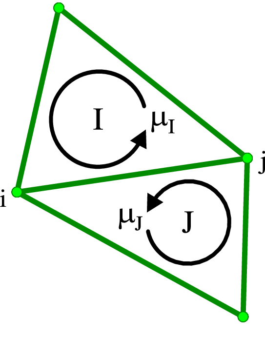
III.1.4 Full heat current

Averaging Eq. (37) or (45) over the system and adding the magnetization contribution Eq. (51) gives the full average heat current density in the $x$ -direction

	$\displaystyle\bar{J}^{Q}_{x}=$	$\displaystyle\frac{1}{\Omega}\sum_{\left<{ij}\right>}x_{ji}\frac{1}{2}(V_{i}+V_{j})(I_{ij}^{\text{tot}}-I_{ij}^{\text{tr}})$
	$\displaystyle-$	$\displaystyle\frac{1}{\Omega}\sum_{\left<{IJ}\right>}\left[\left(x_{ij}^{c}-x_{I}\right)\mu_{I}-\left(x_{ij}^{c}-x_{J}\right)\mu_{J}\right]\dot{A}_{ij},$		(52)

where $x_{ji}=x_{j}-x_{i}$ is the $x$ -component of the difference vector from site $i$ to $j$ , $x_{ij}^{c}=(x_{i}+x_{j})/2$ , and $x_{I}$ the plaquette centers (the vertices of the Voronoi graph). In the limit where $\dot{\bf A}$ is spatially uniform the last term simplifies to $-\dot{A}_{y}M_{z}$ , where $M_{z}=\sum_{I}\mu_{I}\Omega_{I}/\Omega$ is the average magnetization density [ $\Omega_{I}$ is the area of the (Voronoi) cell $I$ ], in agreement with Eq. (30). A more practically useful form is obtained below in Sec. III.2.4 by expressing the loop currents $\mu_{I}$ in terms of the total currents $I_{ij}^{\text{tot}}$ , which results in the expression Eq. (25).

III.2 Heat current from Kubo formula

It is useful to see how the heat current enters the linear response arising from an applied temperature gradient via a Kubo formula. We will do this starting from the stochastic equations of motion of either Langevin [Eq. (12)] or RCSJ [Eq. (19)] dynamics. The temperature enters these equations only via the strength of the Gaussian noise correlation function, which now gets a spatial dependence $T(x)=T_{0}-T^{\prime}x$ . ¹¹ 1 In reality the parameters of the model, e.g., $I_{ij}^{C}$ , are going to be temperature dependent and therefore also spatially dependent in a temperature gradient. However, this dependence only changes the equilibrium distribution of the model and does not give rise to a thermodynamic force. We can therefore ignore this temperature dependence in the derivation of the heat current. $T^{\prime}$ is considered a weak perturbation, and we are interested in calculating the response of some dynamical variable $A$ to such a perturbation. We assume open boundary conditions in the $x$ -direction, i.e., in the direction of the applied temperature gradient, while in the transverse $y$ -direction they can be arbitrary. With no net electric current flowing through the sample the heat current is equal to the energy current.

For concreteness we consider the response of the electric field $E_{y}$ perpendicular to the temperature gradient and the magnetic field, which gives the Nernst signal $e_{N}=\delta\left<{E_{y}}\right>/\delta T^{\prime}$ . Our goal is to express this linear response using a Kubo formula

e_{N}=\frac{\Omega}{T^{2}}\int_{0}^{\infty}\left<{\bar{E}_{y}(t)\bar{J}_{x}^{Q}(0)}\right>dt,

(53)

where $\bar{J}_{x}^{Q}$ then can be identified with the heat current (the overbar denotes a spatial average), and $\Omega=L_{x}L_{y}$ is the system size.

To this end is convenient to reformulate the problem using functional integrals [40] and write ensemble averages as

\left<{A(t)}\right>=\frac{1}{Z}\int A(\theta(t))e^{-S[\theta]}J[\theta][d\theta],

(54)

where $e^{-S}$ is the statistical weight of a given realization of the stochastic process $\theta(t)$ . The Jacobian $J[\theta]$ in Eq. (54) comes from the transformation from the Gaussian noise $\zeta$ to $\theta$ [40], but since it plays no role in the following it will be dropped henceforth. The linear response of $A$ to a temperature gradient can now be expressed (assuming time translation invariance) as

R(t-t^{\prime})=\frac{\delta\left<{A(t)}\right>}{\delta T^{\prime}(t^{\prime})}=\left<{A(t)Q(t^{\prime})}\right>,

(55)

where

Q(t^{\prime})=-\left.\frac{\delta S[\theta]}{\delta T^{\prime}(t^{\prime})}\right|_{T^{\prime}=0}.

(56)

We are interested in the response to a static perturbation in a stationary state given by

R=\int_{-\infty}^{\infty}\left<{A(t)Q(0)}\right>dt.

(57)

Despite the similarity with Eq. (53), we cannot immediately identify $2T^{2}Q(t)/\Omega$ with $J^{Q}(t)$ at this stage, because of their different symmetry properties, an issue we now digress into.

III.2.1 Symmetry relations of transport coefficients and correlation functions

Before continuing the derivation of the heat current from the Kubo formula we discuss some general properties of linear response in classical statistical systems. It is well known that time reversal symmetry implies symmetry relations among the transport coefficients and among correlation functions. In the presence of a magnetic field $H$ the time reversal operation should reverse also that. Consider now the correlation function $C_{E_{y}Q}(t,H)=\left<{E_{y}(t)Q(0)}\right>$ entering Eq. (55), which in general also depends on the magnetic field $H$ . The electric field $E_{y}$ is even under time reversal, while $Q$ is neither even nor odd. Instead we may split $Q=Q_{e}+Q_{o}$ into even and odd parts. By parity symmetry the correlation functions $C_{E_{y}Q_{e,o}}$ are odd in $H$ , so that

	$\displaystyle\!\!C_{E_{y}Q_{e}}(t,H)$	$\displaystyle=C_{E_{y}Q_{e}}(-t,-H)=-C_{E_{y}Q_{e}}(-t,H),$		(58)
	$\displaystyle\!\!C_{E_{y}Q_{o}}(t,H)$	$\displaystyle=-C_{E_{y}Q_{o}}(-t,-H)=C_{E_{y}Q_{o}}(-t,H).$		(59)

This leads to the following symmetry of the response

	$\displaystyle R(t,H)$	$\displaystyle=C_{E_{y}Q_{e}}(t,H)+C_{E_{y}Q_{o}}(t,H)$
		$\displaystyle=-C_{E_{y}Q_{e}}(-t,H)+C_{E_{y}Q_{o}}(-t,H).$		(60)

For $t<0$ causality implies that $R(t,H)=0$ , hence $C_{E_{y}Q_{o}}(-t,H)=C_{E_{y}Q_{e}}(-t,H)$ , so that the response can be written solely in terms of the odd part of $Q$ as

R(t,H)=2\Theta(t)C_{E_{y}Q_{o}}(t,H),

(61)

where $\Theta(t)$ is the Heaviside step function. For the Nernst signal we then get

e_{N}=\int_{0}^{\infty}2C_{E_{y}Q_{o}}(t)dt=\int_{-\infty}^{\infty}\left<{E_{y}(t)Q_{o}(0)}\right>dt.

(62)

Thus, in order to evaluate the response it is enough to consider the odd part of $Q(t)$ .

Let us also make the following observation: At finite times the response will contain transients, which we will not be interested in and which do not contribute to the stationary response. Indeed, any contribution to $Q_{o}(t)$ of the form of a total time derivative $df/dt$ will contribute a term

\int_{-\infty}^{\infty}\langle E_{y}(0)\frac{df(t)}{dt}\rangle dt=\left<{E_{y}(0)f(\infty)}\right>-\left<{E_{y}(0)f(-\infty)}\right>

(63)

to $e_{N}$ , which vanishes provided $f(t)$ is stationary in equilibrium. We will now treat the Langevin and RCSJ case separately.

III.2.2 Langevin dynamics

For the case of Langevin dynamics the dynamical action $S$ obtains from substituting $\eta$ using Eq. (12) in the Gaussian noise probability distribution

P[\eta]\propto\exp\big(-\int\sum_{i}\frac{\hbar}{4\gamma T_{i}}\eta_{i}^{2}(t)dt\big)

(64)

resulting in

S_{\text{Lang.}}=\int\sum_{i}\frac{\hbar}{4\gamma T_{i}}\left(\gamma\dot{\theta}_{i}-F_{i}\right)^{2}dt,

(65)

where

F_{i}=-\frac{1}{\hbar}\frac{\partial H}{\partial\theta_{i}}=-\frac{1}{2e}\sum_{j\in\mathcal{N}_{i}}I_{ij}^{s},

(66)

and correspondingly

Q(t)=-\sum_{i}\frac{\hbar x_{i}}{4\gamma T^{2}}\left(\gamma\dot{\theta}_{i}(t)-F_{i}(t)\right)^{2}.

(67)

Since $\dot{\theta}_{i}=2eV_{i}/\hbar$ is even and $I_{ij}^{s}$ is odd under time reversal ²² 2 $\theta$ changes sign under time reversal, the odd part of $Q$ is

$\displaystyle Q_{o}(t)$	$\displaystyle=\frac{1}{2T^{2}}\sum_{i}x_{i}\hbar\dot{\theta}_{i}F_{i}$
	$\displaystyle=-\frac{1}{2T^{2}}\frac{\hbar}{2e}\sum_{i}x_{i}\dot{\theta}_{i}\sum_{j\in\mathcal{N}_{i}}I_{ij}^{s}$
	$\displaystyle=-\frac{1}{2T^{2}}\frac{\hbar}{2e}\sum_{\left<{ij}\right>}(x_{i}\dot{\theta}_{i}-x_{j}\dot{\theta}_{j})I_{ij}^{s}.$	(68)

Putting $x_{ij}^{c}=(x_{i}+x_{j})/2$ we may rewrite this as

	$\displaystyle 2T^{2}Q_{o}(t)=$	$\displaystyle-\sum_{\left<{ij}\right>}x_{ij}^{c}(V_{i}-V_{j}-\dot{A}_{ij})I_{ij}^{s}$
		$\displaystyle+\sum_{\left<{ij}\right>}\left(\frac{1}{2}x_{ji}(V_{i}+V_{j})-x_{ij}^{c}\dot{A}_{ij}\right)I_{ij}^{s}.$		(69)

The first term is a total time derivative of $x_{ij}^{c}$ times a local energy $e_{ij}$

\frac{d}{dt}\sum_{\left<{ij}\right>}x_{ij}^{c}e_{ij}=-\sum_{\left<{ij}\right>}x_{ij}^{c}\frac{d}{dt}J_{ij}\cos\gamma_{ij},

(70)

and will therefore not contribute to static response functions. The remaining part can be identified with the heat current in the Langevin model,

\bar{J}^{Q}_{x}=\frac{1}{\Omega}\sum_{\left<{ij}\right>}\left(\frac{1}{2}x_{ji}(V_{i}+V_{j})-x_{ij}^{c}\dot{A}_{ij}\right)I_{ij}^{s}.

(71)

This form of the heat current is directly formulated using the currents and potentials, and therefore simpler to use than Eq. (52). To show the equivalence of Eqs. (71) and (52) it is necessary to go through some further steps. Before doing that, however, we consider the RCSJ case.

III.2.3 RCSJ dynamics

It is convenient to reformulate the equations of motions for RCSJ dynamics Eq. (19) as

		$\displaystyle I_{ij}^{\text{tot}}=I_{ij}^{C}+I_{ij}^{s}+I_{ij}^{R}+I_{ij}^{n}=I_{ij}^{\text{tr}}+\lambda_{i}-\lambda_{j}+\mu_{ij},$		(72)
		$\displaystyle\sum_{j\in\mathcal{N}_{i}}\lambda_{i}-\lambda_{j}=C_{0}\dot{V}_{i},$		(73)

where $\lambda_{i}-\lambda_{j}$ is the longitudinal part of the total current flowing through the links of the lattice, and $\mu_{ij}=\mu_{I}-\mu_{J}$ is the transverse part, with the $\mu_{I}$ defined on the dual lattice sites, i.e., on the plaquettes, adjacent to the bond $ij$ as in Fig. 4. The $\mu_{I}$ :s are often referred to as loop currents. Neither of these contribute to the transport current $I_{ij}^{\text{tr}}$ . As in the Langevin case we set $I_{ij}^{\text{tr}}=0$ , whereby the heat current equals the energy current.

The dynamical action corresponding to Eqs. (72–73) can be expressed as

S^{\prime}_{\text{RCSJ}}=\int\sum_{\left<{ij}\right>}\Big\{\frac{R_{ij}}{4T_{ij}}(I_{ij}^{n})^{2}+i\eta_{ij}(I_{ij}^{\text{tot}}-\lambda_{i}+\lambda_{j}-\mu_{ij})\Big\}dt.

(74)

The first term represents the Gaussian distribution of the white noise current $I_{ij}^{n}$ , and $\eta_{ij}$ is a Lagrange multiplier to enforce the constraints Eq. (72). In a temperature gradient the local temperatures are position dependent, $T_{ij}=T-T^{\prime}x_{ij}^{c}$ .

The functional integration is over the variables $\theta$ , $I_{ij}^{n}$ , $\eta_{ij}$ , $\lambda_{i}$ , and $\mu_{I}$ . Integrating over $I_{ij}^{n}$ and $\eta_{ij}$ we get

S_{\text{RCSJ}}=\int\sum_{\left<{ij}\right>}\frac{R_{ij}}{4T_{ij}}(I_{ij}^{C}+I_{ij}^{s}+I_{ij}^{R}-\lambda_{i}+\lambda_{j}-\mu_{ij})^{2}dt,

(75)

and

Q(t)=-\frac{1}{4T^{2}}\sum_{\left<{ij}\right>}x_{ij}^{c}R_{ij}(I_{ij}^{C}+I_{ij}^{s}+I_{ij}^{R}-\lambda_{i}+\lambda_{j}-\mu_{ij})^{2}.

(76)

Again only the part which is odd under time reversal contributes to the heat current,

2T^{2}Q_{o}=-\sum_{\left<{ij}\right>}x_{ij}^{c}V_{ij}\left(I_{ij}^{C}+I_{ij}^{s}-\lambda_{i}+\lambda_{j}-\mu_{ij}\right),

(77)

since $I_{ij}^{R}=V_{ij}/R_{ij}$ is even, while the other currents are odd. In this expression we may identify a contribution

\sum_{\left<{ij}\right>}x_{ij}^{c}V_{ij}(I_{ij}^{C}+I_{ij}^{s})=\frac{d}{dt}\sum_{\left<{ij}\right>}x_{ij}^{c}e_{ij},

(78)

where

e_{ij}=\frac{1}{2}C_{ij}V_{ij}^{2}-J_{ij}\cos(\theta_{i}-\theta_{j}-\frac{2\pi}{\Phi_{0}}A_{ij})

(79)

is the local energy defined on the links of the lattice. Being a total time derivative this does not contribute in a stationary state. The remaining part can be rearranged into

		$\displaystyle\sum_{\left<{ij}\right>}x_{ij}^{c}V_{ij}\left(\lambda_{i}-\lambda_{j}+\mu_{ij}\right)$
		$\displaystyle=\sum_{i}x_{i}V_{i}\sum_{j\in\mathcal{N}_{i}}\left(\lambda_{i}-\lambda_{j}+\mu_{ij}\right)$
		$\displaystyle+\sum_{\left<{ij}\right>}\left[x_{ji}\frac{1}{2}(V_{i}+V_{j})-x_{ij}^{c}\dot{A}_{ij}\right]\left(\lambda_{i}-\lambda_{j}+\mu_{ij}\right).$

The second line equals $\sum_{i}x_{i}C_{0}V_{i}\dot{V}_{i}=\frac{d}{dt}\sum_{i}x_{i}\frac{1}{2}C_{0}V_{i}^{2}$ , again a total time derivative which does not contribute. Finally, $\lambda_{i}-\lambda_{j}+\mu_{ij}=I_{ij}^{\text{tot}}$ , so that the heat current for the RCSJ model becomes

\bar{J}^{Q}_{x}=\frac{1}{\Omega}\sum_{\left<{ij}\right>}\left(x_{ji}\frac{1}{2}(V_{i}+V_{j})-x_{ij}^{c}\dot{A}_{ij}\right)I_{ij}^{\text{tot}}.

(80)

III.2.4 Magnetization contribution

Equations (52) and (71), (80) apparently differ. We will now show the equivalence of these formulations. We split the current into transverse and longitudinal parts as in Eq. (46), with the $\mu_{I}$ defined on the dual lattice, whose sites are denoted by ${\bf r}_{I}=(x_{I},y_{I})$ . With this it is possible to rewrite the last term in Eqs. (71), (80), as

	$\displaystyle-\sum_{\left<{ij}\right>}x_{ij}^{c}\dot{A}_{ij}I_{ij}^{\text{tot}}=-\sum_{\left<{ij}\right>}x_{ij}^{c}\dot{A}_{ij}(\lambda_{i}-\lambda_{j}+\mu_{ij})$
	$\displaystyle=-\sum_{\left<{ij}\right>}x_{ij}^{c}\dot{A}_{ij}(\lambda_{i}-\lambda_{j})-\sum_{I}x_{I}\mu_{I}\sum_{J\in\mathcal{N}_{I}}\dot{A}_{ij}$
	$\displaystyle-\sum_{\left<{IJ}\right>}\left[\left(x_{ij}^{c}-x_{I}\right)\mu_{I}-\left(x_{ij}^{c}-x_{J}\right)\mu_{J}\right]\dot{A}_{ij}.$

The first term is a total time derivative of $\sum_{\left<{ij}\right>}x_{ij}^{c}e_{ij}^{M}$ , where $e_{ij}^{M}=\frac{1}{2}A_{ij}(\lambda_{i}-\lambda_{j})$ is the local magnetization energy of the loops to ground [cf. Eq. (49)]. The second term is a total time derivative of $\sum_{I}x_{I}e_{I}^{M}$ , involving the magnetization energy $e_{I}^{M}=\frac{1}{2}\mu_{I}\Phi_{I}$ of the loops of the lattice. The remaining part corresponds exactly to the last term of Eq. (52). Note that for the models discussed initially $\dot{\bf A}=(\Phi_{0}/2\pi)\dot{\mathbf{\Delta}}$ , i.e., only spatially uniform fluctuations are included in the vector potential. Then $\dot{e}_{ij}^{M}=\dot{e}_{I}=0$ exactly, and Eqs. (52) and (71), (80) become identical (for open boundary conditions). In the more general case where local fluctuations are allowed they differ only by a total time derivative, which does not contribute to the transport coefficients.

III.3 Additional remarks

The two derivations of the heat current given in Sec. III.1 and III.2 above agree. The latter one shows, in addition, the validity of the standard Kubo formula Eq. (22) for calculating the Nernst response of the transverse electric field to an applied temperature gradient (in absence of an electric transport current). The resulting expression should also give, via an Onsager relation, the response of the heat current to an applied transverse electric current. This holds provided the electric transport current $I_{ij}^{\text{tr}}$ is subtracted from the current in Eqs. (71), (80), showing that Eq. (25) is indeed the correct form.

In both the Langevin and the RCSJ case the heat current is given by similar expressions, but in the RCSJ case the current $I_{ij}^{\text{tot}}$ includes also capacitative, resistive, and noise currents in addition to the supercurrent.

As mentioned, Eq. (25), being directly formulated in the currents and phases, have a clear advantage over (52). They are equivalent for systems with open boundary conditions along the temperature gradient. In simulations periodic boundary conditions are convenient to use in order to eliminate surface effects. This, however, makes things more subtle as then the magnetization is not uniquely determined by the currents: Adding a constant to every $\mu_{I}$ does not change $I_{ij}^{\text{tot}}$ in Eq. (46). One logical possibility seems to be to impose an extra condition on the average magnetization, e.g., define it to be zero at any moment, or $\sum_{I}\mu_{I}=0$ , so that no magnetization contribution should be added in this case. Another option is to fix one particular $\mu_{I}$ , and in effect use Eq. (25) also for periodic boundary conditions. We opt for this latter condition, since it stays closer to the experimental open system situation, while getting rid of surface effects. This choice can be further justified by comparing analytic results for open and periodic boundary conditions obtained in a spin wave approximation, to be discussed next.

IV Heat conductivity at low temperature and zero magnetic field

At low enough temperatures and zero magnetic field the fluctuations will be small so that it is sufficient to consider linearized versions of the models introduced earlier. The only nonlinear circuit element is the Josephson junction, and by linearizing the Josephson relation $I_{ij}^{s}=I_{ij}^{c}\sin\gamma_{ij}\approx I_{ij}^{c}\gamma_{ij}$ , the models are reduced to a network of capacitors, resistors and inductors, with effective inductances $\mathcal{L}_{ij}=(\hbar/2eI_{ij}^{c})$ . In this spin wave approximation vortices are absent, hence there will be no Nernst effect, but the thermal conductivity will still be nonzero. For the Langevin case the resulting model can be mapped to one of heat conduction by phonons in a harmonic crystal coupled to local heat baths, which has an analytic solution [37]. For a 2D infinite square lattice the spin wave heat conductivity is independent of temperature and given by

	$\displaystyle\kappa_{\text{sw}}$	$\displaystyle=\frac{k_{B}I_{c}}{2e\gamma}\int_{0}^{1}\int_{0}^{1}\frac{\sin^{2}(\pi x)}{4\sin^{2}(\frac{\pi x}{2})+4\sin^{2}(\frac{\pi y}{2})}dxdy$
		$\displaystyle=(\frac{1}{2}-\frac{1}{\pi})\frac{k_{B}I_{c}}{2e\gamma}\approx 0.1817\frac{k_{B}I_{c}}{2e\gamma}.$		(81)

We now turn to the heat conductivity of the linearized RCSJ model on a 2D square array of size $\Omega=L_{x}L_{y}$ and unit lattice constant. In this case, the heat current [Eq. (80)] includes the total current $I_{ij}^{\text{tot}}=I_{ij}^{C}+I_{ij}^{R}+I_{ij}^{s}+I_{ij}^{n}$ , which is purely transverse due to Eqs. (19) and (20). In this sum, $I_{ij}^{C}$ and $I_{ij}^{R}$ have no transverse component, so that $I_{ij}^{\text{tot}}=I^{s\perp}_{ij}+I^{n\perp}_{ij}$ . The transverse part of the supercurrent $I^{s\perp}_{ij}$ is entirely due to vortices and vanishes in the spin wave approximation, so that the total current only consists of the transverse component of the noise current, $I_{ij}^{\text{tot}}=I^{n\perp}_{ij}$ . More explicitly, this result can be derived from the equations of motion. On a square lattice it is convenient to label the links by the coordinate ${\bf r}$ and direction $\mu=x,y$ , and introduce forward and backward difference operators $\nabla_{\mu}f({\bf r})=\overline{\nabla}_{\mu}f({\bf r}+\hat{\bm{\mu}})=f({\bf r}+\hat{\bm{\mu}})-f({\bf r})$ . Introducing rescaled variables $\phi_{i}=\hbar\theta_{i}/2e$ and $\tilde{\Delta}=\hbar\Delta/2e$ the equations of motion (19), (20) are in this limit

	$\displaystyle\sum_{\mu}\overline{\nabla}_{\mu}\nabla_{\mu}\left(C\ddot{\phi}_{\bf r}+\frac{1}{R}\dot{\phi}_{\bf r}+\frac{1}{\mathcal{L}}\phi_{\bf r}\right)$	$\displaystyle=\sum_{\mu}\overline{\nabla}_{\mu}I^{n}_{{\bf r}\mu},$		(82)
	$\displaystyle C\ddot{\tilde{\Delta}}_{\mu}+\frac{1}{R}\dot{\tilde{\Delta}}_{\mu}+\frac{1}{\mathcal{L}}\tilde{\Delta}_{\mu}$	$\displaystyle=\frac{1}{\Omega}\sum_{{\bf r}}I^{n}_{{\bf r}\mu}.$		(83)

Multiplying Eq. (82) with the lattice Green’s function $G$ (solving $-\overline{\nabla}\nabla G_{{\bf r}{\bf r}^{\prime}}=\delta_{{\bf r},{\bf r}^{\prime}}$ ) gives

C\ddot{\phi}_{\bf r}+\frac{1}{R}\dot{\phi}_{\bf r}+\frac{1}{\mathcal{L}}\phi_{\bf r}=-\sum_{{\bf r}^{\prime}\nu}G_{{\bf r}{\bf r}^{\prime}}\overline{\nabla}_{\nu}I^{n}_{{\bf r}^{\prime}\nu}.

(84)

Using (84) and (83), the total current on a square lattice is

	$\displaystyle I_{{\bf r}\mu}^{\text{tot}}$	$\displaystyle=I_{{\bf r}\mu}^{C}+I_{{\bf r}\mu}^{R}+I_{{\bf r}\mu}^{s}+I_{{\bf r}\mu}^{n}$
		$\displaystyle=I_{{\bf r}\mu}^{n}+\sum_{{\bf r}^{\prime}\nu}\nabla_{\mu}G_{{\bf r}{\bf r}^{\prime}}\overline{\nabla}_{\nu}I^{n}_{{\bf r}^{\prime}\nu}-\frac{1}{\Omega}\sum_{{\bf r}^{\prime}}I^{n}_{{\bf r}^{\prime}\mu}.$		(85)

We can here identify the longitudinal part of the noise current $I^{n\parallel}_{{\bf r}\mu}=-\sum_{{\bf r}^{\prime}\nu}\nabla_{\mu}G_{{\bf r}{\bf r}^{\prime}}\overline{\nabla}_{\nu}I^{n}_{{\bf r}^{\prime}\nu}$ , and the average ( ${\bf k}=0$ component) $I_{\mu}^{n0}=\frac{1}{\Omega}\sum_{{\bf r}}I^{n}_{{\bf r}\mu}$ . The total current is thus just the transverse part of the noise current

I_{{\bf r}\mu}^{\text{tot}}=I^{n}_{{\bf r}\mu}-I^{n\parallel}_{{\bf r}\mu}-I_{\mu}^{n0}=I^{n\perp}_{{\bf r}\mu}.

(86)

The heat current in the $x$ -direction can then be written as

	$\displaystyle\bar{J}^{Q}_{x}$	$\displaystyle=\frac{1}{\Omega}\sum_{{\bf r}\nu}\chi_{{\bf r}\nu}I^{n\perp}_{{\bf r}\nu},$		(87)
	$\displaystyle\chi_{{\bf r}\nu}$	$\displaystyle=\frac{1}{2}(\dot{\phi}_{\bf r}+\dot{\phi}_{{\bf r}+\hat{{\bf x}}})\delta_{\nu x}-(x+\frac{1}{2}\delta_{\nu x})\dot{\tilde{\Delta}}_{\nu}.$		(88)

This result is intriguing because the dynamics of the system is completely independent of $I^{n\perp}_{{\bf r}\mu}$ , as seen from the equations of motion. Correspondingly, the correlation function which enters the Kubo formula Eq. (23) factorizes:

		$\displaystyle\left<{\bar{J}^{Q}_{x}(t)\bar{J}^{Q}_{x}(0)}\right>=\frac{1}{\Omega^{2}}\sum_{{\bf r}\mu,{\bf r}^{\prime}\nu}\left<{\chi_{{\bf r}\mu}(t)I^{n\perp}_{{\bf r}\mu}(t)\chi_{{\bf r}^{\prime}\nu}(0)I^{n\perp}_{{\bf r}^{\prime}\nu}(0)}\right>$
		$\displaystyle\qquad=\frac{1}{\Omega^{2}}\sum_{{\bf r}\mu,{\bf r}^{\prime}\nu}\left<{\chi_{{\bf r}\mu}(t)\chi_{{\bf r}^{\prime}\nu}(0)}\right>\left<{I^{n\perp}_{{\bf r}\mu}(t)I^{n\perp}_{{\bf r}^{\prime}\nu}(0)}\right>.$		(89)

Furthermore, the transverse noise current correlation function

\big<I^{n\perp}_{{\bf r}\mu}(t)I^{n\perp}_{{\bf r}^{\prime}\nu}(0)\big>\\ =\frac{2k_{B}T}{R}\delta(t)\frac{1}{\Omega}\sum_{{\bf k}\neq 0}\left(\delta_{\mu\nu}-\frac{K_{\mu}K_{\nu}}{K^{2}}\right)e^{i{\bf k}\cdot({\bf r}-{\bf r}^{\prime})},

(90)

where $K_{\mu}=2\sin(k_{\mu}/2)$ , $K^{2}=\sum_{\mu}K_{\mu}^{2}$ , $k_{\mu}=2\pi n_{\mu}/L_{\mu}$ , and $n_{\mu}=0,\ldots,L_{\mu}-1$ . Since this is proportional to $\delta(t)$ , the correlation function $\left<{\chi(t)\chi(0)}\right>$ has to be evaluated at $t=0$ when inserted into the Kubo formula, i.e., it is given by an equilibrium correlation function.

In the more general case the total current contains also the transverse part of the supercurrent, which is determined by the vortices. Clearly the vortex contribution appears on top of the spin wave background calculated in this section. We may evaluate the correlation function $\left<{\chi_{{\bf r}\mu}\chi_{{\bf r}^{\prime}\nu}}\right>$ for the full model, including a capacitance $C_{0}$ to ground and cosine interaction. On a square lattice the RCSJ Hamiltonian Eq. (38) is

H=\sum_{\bf r}\frac{1}{2}C_{0}V_{\bf r}^{2}+\sum_{{\bf r},\mu}\frac{1}{2}C(V_{\bf r}-V_{{\bf r}+\hat{\mu}}-\dot{\tilde{\Delta}}_{\mu})^{2}+f(\phi,\tilde{\bm{\Delta}}),

(91)

where $V_{\bf r}=\dot{\phi}_{\bf r}$ and $f(\phi,\tilde{\bm{\Delta}})$ is the “potential energy” involving the cosine interaction. Switching to Fourier space

H=\frac{1}{\Omega}\sum_{\bf k}\frac{1}{2}(C_{0}+CK^{2})V_{-{\bf k}}V_{{\bf k}}+\frac{1}{2}C\Omega(\dot{\tilde{\Delta}}_{x}^{2}+\dot{\tilde{\Delta}}_{y}^{2})+f(\phi,\tilde{\bm{\Delta}}).

(92)

From here it is easy to calculate the required averages, since the partition function factorizes at the classical level and the averages are just Gaussian integrals. We get

\left<{V_{-{\bf k}}V_{{\bf k}}}\right>=\frac{k_{B}T}{C_{0}+CK^{2}},\qquad\big<\dot{\Delta}_{\mu}\dot{\Delta}_{\nu}\big>=\frac{k_{B}T}{C\Omega}\delta_{\mu\nu},

(93)

independent of $f(\phi,\tilde{\bm{\Delta}})$ , so that

$\displaystyle\left<{\chi_{{\bf r}x}\chi_{{\bf r}^{\prime}x}}\right>$	$\displaystyle=\frac{1}{\Omega}\sum_{\bf k}e^{i{\bf k}\cdot({\bf r}-{\bf r}^{\prime})}\frac{1}{4}\left\|1+e^{ik_{x}}\right\|^{2}\left<{V_{\bf k}V_{-{\bf k}}}\right>$
	$\displaystyle+\Big(x+\frac{1}{2}\Big)\Big(x^{\prime}+\frac{1}{2}\Big)\left<{\dot{\tilde{\Delta}}_{x}\dot{\tilde{\Delta}}_{x}}\right>,$	(94)
$\displaystyle\left<{\chi_{{\bf r}y}\chi_{{\bf r}^{\prime}y}}\right>$	$\displaystyle=xx^{\prime}\left<{\dot{\tilde{\Delta}}_{y}\dot{\tilde{\Delta}}_{y}}\right>,$	(95)
$\displaystyle\left<{\chi_{{\bf r}x}\chi_{{\bf r}^{\prime}y}}\right>$	$\displaystyle=\left<{\chi_{{\bf r}y}\chi_{{\bf r}^{\prime}x}}\right>=0.$	(96)

Performing the sum over ${\bf r},{\bf r}^{\prime}$ in (89) and using (90), (93)–(96) the heat conductivity becomes

$\displaystyle\kappa_{\text{sw}}$	$\displaystyle=\kappa^{\prime}+\kappa^{\prime\prime},$	(97)
$\displaystyle\kappa^{\prime}$	$\displaystyle=\frac{k_{B}}{RC}\frac{1}{\Omega}\sum_{{\bf k}\neq 0}\frac{\left(1+\frac{1}{4}K_{x}^{2}\right)\left(1-\frac{K_{x}^{2}}{K^{2}}\right)}{C_{0}/C+K^{2}},$	(98)
$\displaystyle\kappa^{\prime\prime}$	$\displaystyle=\frac{k_{B}}{RC}\frac{L_{x}^{2}-1}{12\Omega}.$	(99)

The second term $\kappa^{\prime\prime}$ originates from $\langle\dot{\tilde{\Delta}}_{y}\dot{\tilde{\Delta}}_{y}\rangle$ and corresponds to the magnetization contribution.

The resulting heat conductivity Eq. (97) has some notable properties. Firstly, it is proportional to $1/RC$ so that it is well defined only for finite $C$ . In this respect the RSJ model, without shunting capacitors, i.e., with $C\to 0$ is pathological. Secondly, when $C_{0}=0$ the sum over ${\bf k}$ in (98) is logarithmically divergent in the infinite system $L\to\infty$ (in 2D). For finite large $L$ the heat conductivity has a logarithmic size dependence

\kappa_{\text{sw}}\sim\frac{1}{4\pi RC}\ln\frac{L}{a},

(100)

where $a$ is the lattice spacing. $\kappa$ is thus not a bulk property of the RCSJ model in 2D. It is interesting to note that several other low dimensional models of heat conduction display an anomalous size dependence, often tied to momentum conservation [42, 43]. In the present case the diverging behavior is most likely due to the long range Coulomb interaction. A finite $C_{0}$ makes the charge-charge interaction exponentially small on distances larger than the screening length $\lambda=a\sqrt{C/C_{0}}$ , and also yields a system size independent $\kappa_{\text{sw}}$ when $L\gg\lambda$ . The calculation above was done for periodic boundary conditions. We have repeated it for open boundary conditions in the $x$ -direction. The difference is very small and tends to zero as $1/L_{x}$ when $L_{x}$ increases.

As discussed above, the vortex contribution appears on top of the temperature independent spin wave background just calculated. Computationally it is often convenient to project out the spin wave contribution by excluding the transverse noise current $I^{n\perp}$ in Eq. (52) before the averaging in Eq. (23).

V Simulation methods

The equations of motion for Langevin dynamics [Eq. (12) and Eq. (13)] are solved numerically using a simple forward Euler discretization with a time step of $\Delta t=0.02$ . The RCSJ dynamical equations [Eq. (19) and Eq. (20)] have a more complicated structure and are also second order in time, which makes the solution numerically more intensive. To solve these we use a leap-frog type discretization scheme, with time step $\Delta t=0.04$ . For a system of $N$ grains one then generally has to solve a system of $N+1$ coupled equations in each time step ( $N-1$ for the phases $\{\theta_{i}\}$ and 2 for the twists $\bm{\Delta}$ ). Note, however, that the equation system is sparse, so an effective way to solve them is to employ an LU factorization algorithm, since the complexity of such a scheme goes as the number of nonzero entries, which are of the order of $N$ here. This is far better than the direct method [23, 24] of multiplying with the lattice Green’s function, which is here a dense matrix with $\sim N^{2}$ nonzero entries. In both the Langevin and the RCSJ case the sampling is performed during $4\cdot 10^{5}$ units of time, after an equilibration time of 10% of this.

We have simulated systems of sizes up to $120\times 120$ , but except the case of $\kappa$ for RCSJ dynamics, finite size effects are unimportant for systems larger than $L\gtrsim 20$ , and thus only systems of size $20\times 20$ are considered.

The transport coefficients are calculated from the Kubo formulas Eqs. (22)-(24), where the upper limit in the time integrals is replaced by a large enough time ( $\gtrsim$ the correlation time), such that the cumulative value of the integral has stabilized its value. The Nernst signal $e_{N}$ obtained from the Kubo formula in Eq. (22) is also compared with the value of $e_{N}$ calculated in two other ways. The first is simply to apply a small temperature gradient in the $x$ -direction and measure the resulting electric field $E_{y}$ , and the second is through the Onsager relation $e_{N}=\tilde{\beta}_{xy}/T$ , where $\tilde{\beta}$ is the response of the heat current in the $x$ -direction to an applied electric current in the $y$ -direction, as defined in Eq. (5). This gives an important consistency check of our calculations. A similar check is performed for the heat conductivity $\kappa$ . The Kubo formula turns out to be the most efficient way to calculate the response, since one does not have to worry about nonlinear effects.

V.1 Units

In the simulations we redefine time and temperature to make them dimensionless (we also measure length in units of a lattice constant $a$ ). For both Langevin and RCSJ dynamics, temperature is rescaled according to

T\to T\frac{2ek_{B}}{\hbar I^{c}}.

(101)

The dimensionless time is obtained from the transformation

t\to t\frac{I^{c}}{2e\gamma},

(102)

for Langevin dynamics. In the RCSJ case the rescaling is

t\to t\frac{2eRI^{c}}{\hbar}.

(103)

(In the case where the junction parameters vary from link to link $I^{c}$ , $R$ and $C$ denote a characteristic magnitude.) From this follows that for Langevin dynamics, the Nernst signal $e_{N}$ is given in units of $k_{B}/2e\gamma$ , the thermal conductivity $\kappa$ in units of $k_{B}I^{c}/2e\gamma$ , and the resistivity $\rho$ in units of $\hbar/(2e)^{2}\gamma$ . For RCSJ dynamics the Nernst signal $e_{N}$ is measured in units of $2ek_{B}R/\hbar$ , the thermal conductivity $\kappa$ in units of $2ek_{B}RI^{c}/\hbar$ , and the resistivity $\rho$ in units of the shunt resistance $R$ . The dimensionless parameter $Q^{2}=2eR^{2}I^{c}C/\hbar$ (the ratio of the two times scales $RC$ and $\hbar/2eRI^{c}$ ) controls the damping. For $Q\gg 1$ the system is underdamped and for $Q\ll 1$ it is overdamped.

V.2 Time discretization of the heat current

It is crucial to use a symmetric time discretization of the heat current, Eq. (25), in the numerics. For Langevin dynamics, while it is sufficient to use a forward Euler discretization for the integration of the equations of motion, the voltage $V_{i}=\hbar\dot{\theta}_{i}/2e$ appearing in Eq. (25) has to be approximated by a centered difference $\dot{\theta}(t)\approx\{\theta(t+\Delta t)-\theta(t-\Delta t)\}/2\Delta t$ . In the RCSJ case the total electric current is (after rescaling time)

I_{ij}^{\text{tot}}(t)=I_{ij}^{c}\left(\sin\gamma_{ij}(t)+\dot{\gamma}_{ij}(t)+Q^{2}\ddot{\gamma}_{ij}(t)\right)+I_{ij}^{n}(t).

(104)

In the symmetric leap-frog scheme we use, $\theta$ is defined on integer time steps $t=n\Delta t$ , while the first order time derivative $\dot{\theta}$ is defined only on half-integer time steps $t=(n+1/2)\Delta t$ , so $\dot{\theta}(t)$ has to be calculated as the average of $\dot{\theta}$ at the two adjacent time steps

\displaystyle\dot{\theta}(t)\approx\frac{1}{2}\big\{\dot{\theta}(t+\Delta t/2)+\dot{\theta}(t-\Delta t/2)\big\}.

(105)

The second order time derivative $\ddot{\theta}(t)$ is symmetrically defined as

\displaystyle\ddot{\theta}(t)\approx\frac{1}{\Delta t}\big\{\dot{\theta}(t+\Delta t/2)-\dot{\theta}(t-\Delta t/2)\big\}.

(106)

The same applies for the twist variables $\mathbf{\Delta}$ . These definitions make the heat current $\bar{J}^{Q}_{x}(t)$ as defined above naturally symmetric around $t$ . An interesting aspect here is that by choosing the time step as $\Delta t=2Q^{2}$ , the RCSJ equations of motion discretized by the symmetric leap-frog scheme actually reduce exactly to the RSJ equations of motion discretized using an asymmetric forward Euler scheme. Moreover $I_{ij}^{\text{tot}}(t)$ becomes the sum of the super-, resistive, and noise currents discretized by a forward Euler scheme as it should for the RSJ model, while the voltages in Eq. (25) are kept symmetric due to the definition Eq. (105). The RSJ model is therefore best thought of as a special case of an overdamped RCSJ model with $Q^{2}=\Delta t/2$ (with our choice of $\Delta t=0.04$ this corresponds to $Q^{2}=0.02$ ).

We find that the heat current $\bar{J}^{Q}_{x}(t)$ is very sensitive to the discretization used. In fact, it is critical to use the symmetric way of defining $\bar{J}^{Q}_{x}(t)$ to obtain consistent results when calculating the heat conductivity $\kappa$ either using a Kubo formula or by applying a small temperature gradient.

VI Results and discussion

VI.1 Zero field thermal conductivity

Figure 5 shows the thermal conductivity $\kappa$ in zero magnetic field for fairly underdamped RCSJ dynamics ( $Q=10$ ) for different system sizes $L$ . At low $T$ it tends to the spin wave value given by Eq. (100), which in dimensionless units becomes $\kappa\sim(1/4\pi Q^{2})\ln(L/a)$ . For large $Q$ this background value is quite small. For smaller values of $Q$ the background increases and soon overwhelms the vortex contribution. In the following it will therefore be subtracted.

The dependence on system size $L$ for low temperatures can be seen in the inset of Fig. 5. The dependence is logarithmic and follows very well the form in Eq. (100), shown as the red curve in the inset. In Fig. 6 we can see $\kappa$ as a function of temperature in the strongly overdamped limit $C\to 0$ (corresponding to RSJ dynamics), but now with the harmonic spin wave background subtracted. In RSJ dynamics where $C=0$ , the spin wave contribution is formally proportional to $\delta(0)$ , which translates to $1/\Delta t$ in the numerics, where $\Delta t$ is the time step used in the discretization (remember that RSJ dynamics with finite timestep $\Delta t$ can be viewed as a special case of RCSJ dynamics with $Q^{2}=\Delta t/2$ ). What is left after subtracting this part can be interpreted as coming mainly from the motion of vortices. The curves of $\kappa$ start out very small for low temperatures, but increase rapidly on approaching the Berezinskii-Kosterlitz-Thouless [20, *Berezinskii2, *KT] temperature $T_{\text{BKT}}\simeq 0.9$ , where the unbinding of thermally induced vortex-antivortex pairs makes a large contribution to the thermal conductivity. At around $T=1.4$ $\kappa$ reaches its maximum value, followed by a slow decrease for higher temperatures. Note that $\kappa$ , even after subtracting the background, shows a logarithmic dependence on the system size. The inset of Fig. 6 displays the curves for different system sizes divided by the factor $\ln(L/a)$ , with $a=0.7$ . The collapse of the curves onto a single one is very good over the entire temperature range (except from very close to $T_{\text{BKT}}\simeq 0.9$ , where small deviations are expectedly seen).

In the spin wave approximation the logarithmic size dependence seems to be related to the long range Coulomb interation. Screening can be introduced by adding capacitances to ground on every grain, which removes the divergent behavior on length scales larger than the screening length $\sqrt{C/C_{0}}$ . In a similar spirit, it seems likely that the logaritmic size dependence of the vortex contribution is tied to the unscreened Coulomb interaction in the RCSJ model.

For Langevin dynamics, on the other hand, $\kappa$ is only weakly dependent on system size and quickly converge to a size independent bulk value (for $L\gtrsim 20$ ). Moreover, the finite size effects of $e_{N}$ and $\rho$ are also negligible for $L\gtrsim 20$ , for both Langevin and RCSJ dynamics. We will therefore stick to lattices of size $20\times 20$ in the remainder of this paper.

At low $T$ for Langevin dynamics (see the lowest curve in the middle panel of Fig. 7) $\kappa$ goes to the spin wave value Eq. (81), but decreases slightly upon increasing the temperature until temperature induced vortices become plentiful near the BKT transition, where $\kappa$ increases again reaching a maximum around $T\approx 1.25$ and then starts to decrease.

VI.2 Low fields

We now turn to the case of a relatively weak applied transverse magnetic field. In Fig. 7 and 8 we see a collection of simulation results for fillings $f=0$ to $0.05$ on a $20\times 20$ square lattice for Langevin and RCSJ dynamics (Q = 0.5) respectively. The filling $f=B\left<{A_{\text{pl}}}\right>/\Phi_{0}$ , where $\left<{A_{\text{pl}}}\right>$ is the average plaquette area, represents the average number of magnetic field induced vortices per plaquette in the system. The lowest nonzero filling $f=0.0025=1/20^{2}$ corresponds to one field induced vortex in the system. Increasing the filling, i.e., raising the magnetic field will cause the vortex density to increase, but as long as the typical vortex separation is much larger than the coherence length $\xi$ ( $\xi$ can be thought of as the short distance cut-off or lattice spacing $a$ in our model) the effects of discreteness are negligible and the model should describe a continuous two-dimensional (or quasi-two-dimensional) type-II superconductor. The case of strong magnetic fields are discussed in Section VI.3.

Focusing on the Nernst signal $e_{N}$ in Fig. 7 and 8, we notice a very steep increase of $e_{N}$ at low temperatures to a maximum between $T=0.10$ and $0.15$ . At higher temperatures $e_{N}$ slowly decreases and the tail persists up to about $T=2$ , which is roughly twice the BKT transition temperature $T_{\text{BKT}}\approx 0.9$ . These features are qualitatively similar for both Langevin and RCSJ dynamics. The main difference between the models in the shape of $e_{N}$ is the plateau-like part of the curves present in the RCSJ case around $T=0.7$ for low fillings. The peak height increases rapidly with filling, before it starts to decrease for higher fillings. The position of the Nernst signal peak depends slightly on the filling $f$ and moves towards higher temperatures for larger fillings.

The qualitative features of the Nernst signal are in agreement with experiments on several superconductors [44, 2, 45, 4]. A detailed comparison is, however, possible only if the temperature and magnetic field dependences of the parameters $\gamma$ , $R$ , $I^{c}$ are taken into account. For Josephson-junction arrays made up of tunnel junctions the Ambegaokar-Baratoff formula [46, *AmbegaokarBaratoff1963b] $I^{c}=(\pi\Delta(T)/2eR)\tanh(\Delta(T)/2k_{B}T)$ can be used. In bulk superconductors $I^{c}$ is proportional to absolute square of the superconducting order parameter $|\psi|^{2}$ , which goes as $\sim(T_{c}^{\text{MF}}-T)$ , near $T_{c}^{\text{MF}}$ . The situation in the high- $T_{c}$ cuprates is more complicated, since a model for the relaxation rate, $\gamma(T)^{-1}$ in the Langevin case, or $R(T)$ in the RCSJ case, is also required. The thermoelectric coefficient $\alpha_{xy}=e_{N}/\rho$ may have an advantage here, since both $e_{N}$ and $\rho$ are proportional to the relaxation rate, which therefore drops out [7, 11]. We will return to $\alpha_{xy}$ in the next subsection.

In the second row of Fig. 7 and 8 the heat conductivity $\kappa$ is plotted as a function of temperature at different fillings $f$ (in the RCSJ case the spin wave background has been subtracted). Note first how similar the low temperature part of the curves of $\kappa$ are to the Nernst signal. The onset and the peak positions of the two quantities agree to a high degree. For Langevin dynamics (Fig. 7) $\kappa$ is finite in the limit $T\to 0$ . For the two lowest fillings $f=0.0025$ and $0.005$ , $\kappa$ increases quickly as a function of $T$ and then falls off slowly below the $T\to 0$ value of $\sim 0.20$ to suddenly increase again around $T_{\text{BKT}}$ and reach a second maximum followed by slow a decrease at higher temperatures. At fillings above $f=0.005$ the thermal conductivity follows the same pattern, but does not fall below the $T\to 0$ value until temperatures above $T_{\text{BKT}}$ . In the high temperature regime $T\gtrsim 1.5$ all curves, regardless of filling $f$ , fall onto a single curve. The curves for overdamped RCSJ dynamics with $Q=0.5$ (Fig. 8) share this feature of two maxima. In this case, however, the falloff after the first maximum is even more pronounced and persists up to higher fillings, at least $f=0.05$ . Note that the temperature independent background contribution to $\kappa$ has been subtracted in this figure.

The double-peak behavior seems to indicate two separate contributions to the thermal conductivity at high and low temperatures. The first maximum at low $T$ is probably caused by the increased mobility of the field induced vortices, which also gives the sharp rise of $e_{N}$ . This contribution diminishes with increasing $T$ , until the unbinding of temperature induced vortex-antivortex pairs around $T_{\text{BKT}}\simeq 0.9$ makes $\kappa$ large again. This latter contribution totally dominates the previous one at higher temperatures, causing curves for different fillings to converge.

Looking at the resistivity $\rho$ , it displays, not the same but a qualitatively similar $T$ dependence, for Langevin and RCSJ dynamics. For Langevin dynamics the effect of varying filling $f$ is somewhat more apparent, and the rise at $T_{\text{BKT}}$ is also a bit steeper than for RCSJ dynamics.

The results for the RCSJ model discussed previously have been for the overdamped case $Q=0.5$ . Upon reducing the damping and moving into the underdamped regime, $e_{N}$ is effectively unchanged in the low temperature region (apart from a trivial change of scale). However, $\kappa$ and $\rho$ change slightly at high temperatures $T\gtrsim 1.5$ , in that $\kappa$ decays somewhat faster and the falloff starts at a lower temperature, while $\rho$ increases more quickly as function of $T$ , than in the underdamped case.

VI.2.1 Vortex heat transport

In our models there is no Hall effect ( $\sigma_{xy}=0$ ), leading to $e_{N}=\alpha_{xy}/\sigma_{xx}=\alpha_{xy}\rho_{xx}$ , and so we can obtain yet another transport coefficient, the off-diagonal component of the thermoelectric tensor $\alpha_{xy}$ from $e_{N}$ and $\rho$ . As mentioned one advantage with $\alpha_{xy}$ is that, unlike $e_{N}$ and $\kappa$ , it does not depend on the time constants $\gamma$ and $R$ [7, 11]. This makes comparison with experimental data easier. Furthermore, from phenomenological theories of vortex motion $\alpha_{xy}$ has the interesting interpretation of the entropy per vortex [48], suggesting that $\alpha_{xy}T$ can be identified with the transported heat per vortex. This can also be seen from the Onsager relation $\tilde{\alpha}_{xy}=\alpha_{xy}T$ together with the definition of the transverse electrothermal conductivity $\tilde{\alpha}_{xy}=J^{Q}_{x}/E_{y}$ , which is measured under conditions with no applied temperature gradient. Now, since $E_{y}$ is proportional to the transverse vortex current $J^{v}_{x}$ through the relation $E_{y}=\Phi_{0}J^{v}_{x}$ , the quantity $J^{Q}_{x}/E_{y}$ is just the ratio between the heat current and the vortex current, i.e., a measure of the average transported heat per vortex.

Another way of calculating the heat transported per vortex, or more precisely the ratio between the heat current and the vortex current, is to simply divide the vortex contribution $\kappa$ of the longitudinal heat conductivity (i.e., with the spin wave background subtracted) with the Nernst signal, $\kappa/e_{N}=(\frac{J^{Q}_{x}}{-\nabla_{x}T})/(\frac{E_{y}}{-\nabla_{x}T})=J^{Q}_{x}/E_{y}$ . Note, however, that in this context the ratio $J^{Q}_{x}/E_{y}$ measures the transported heat per vortex in a system driven by a temperature gradient $\nabla_{x}T$ , as opposed to the case of $\alpha_{xy}T=J^{Q}_{x}/E_{y}$ , where the driving force is a transverse electric current $J_{y}$ . An equality of $\kappa/e_{N}$ and $\alpha_{xy}T$ would imply a strict proportionality of the heat current $J^{Q}_{x}$ on the vortex current $J^{v}_{x}$ .

In Fig. 9 $\kappa/e_{N}$ and $\alpha_{xy}T$ from our simulations are plotted as functions of temperature $T$ . While they are not equal, they do agree very well at low $T$ (and for low fillings $f$ ), so here one can approximately speak about transported heat per vortex. $\kappa/e_{N}$ is consistently larger than $\alpha_{xy}T$ , and the difference grows with increasing $T$ (and increasing $f$ ). A clue to why this happens can be found considering the difference in what drives the vortex motion in the two cases, as mentioned above. When applying a temperature gradient, heat can be transported even without a net flow of vortices, being mediated solely through the interactions between vortices at different temperatures. This is not possible when the driving force is the transverse electric current, and naturally explains why $\kappa/e_{N}$ is always greater than $\alpha_{xy}T$ . The magnetic field (or filling $f$ ) dependence of $\kappa/e_{N}$ and $\alpha_{xy}T$ at a low fixed temperature is shown in the inset of Fig. 9. The plot is in lin-log scale and clearly shows a logarithmic dependence at low fillings, which is quite similar for both quantities. Such a logarithmic dependence obtains from an ideal gas treatment of the vortices, the Sackur-Tetrode entropy per vortex being $\sim-\ln f$ . The vortices are, however, strongly interacting. A crude way to estimate the interaction effects on the transport entropy would be to assume that the available volume per vortex is reduced by a factor of $N$ , the number of vortices. This then gives a contribution $\ln\Omega/N=-\ln f$ to the configurational entropy, i.e., also a logarithmic dependence.

Also notice that in the low temperature region of Fig. 9, up to about $T\simeq 0.5$ , $\kappa/e_{N}$ and $\alpha_{xy}T$ are only weakly temperature dependent. This means that $\alpha_{xy}$ roughly falls of as $\sim 1/T$ for low temperatures. A fit to $\sim 1/T$ of $\alpha_{xy}$ for RCSJ dynamics ( $Q=0.5$ ) at $f=0.01$ is displayed in Fig. 10. The inset in log-log scale reveals that for temperatures above $T\simeq 0.8$ , $\alpha_{xy}$ falls off much faster, somewhere close to $\sim 1/T^{8}$ . These features are valid also for Langevin and RSJ dynamics, as well as for other types of lattices.

VI.3 Intermediate and high fields - effects of granularity

Going to higher magnetic fields the type of lattice structure starts to play an important role, as geometric frustration will affect vortex transport in this regime. The models at hand are then more valid as descriptions of granular superconductors.

VI.3.1 Square lattices

Figures 11 and 12 show simulation results as a function of filling $f$ for Langevin and RSJ dynamics (corresponds to RCSJ dynamics with $Q=\sqrt{0.02}$ ) on a $20\times 20$ square lattice. At low fillings the Nernst signal $e_{N}$ and the heat conductivity $\kappa$ both show a sharp increase culminating in a maximum around $f=0.05-0.15$ , depending on temperature, followed by a decrease up to half-filling. This “tilted-hill” profile of the Nernst signal seems to be generic and is found in a number of experiments on cuprates and ordinary type-II superconductors [1, *WangOng2006, 49]. Note how $e_{N}$ is always zero at $f=0$ and $1/2$ , due to vortex - vacancy symmetry. The heat conductivity $\kappa$ on the other hand stays finite at $f=1/2$ . On a perfectly periodic lattice all physical quantities are, because of the symmetry of the XY model Hamiltonian [Eq. (11)], periodic in filling $f$ , with period one, and also mirror symmetric (for $\rho$ , $\kappa$ ) or antisymmetric ( $e_{N}$ ) around $f=1/2$ . Thus, all information is contained in the region $f=0\to 0.5$ , which is displayed here.

Now, lowering the temperature the curves have significant structure due to geometric frustration as the filling is varied through different commensurate values. At fillings such as $f$ = 1/8, 1/5, 1/3, 2/5, all three transport coefficients $e_{N}$ , $\kappa$ and $\rho$ are reduced due to vortex pinning to the underlying lattice. This is particularly apparent at the 2nd lowest temperature $T=0.2$ (cyan colored curves) at f = 1/3 and 2/5. The observant reader may also have noticed that the Nernst signal actually goes negative in a region below half-filling. In fact a small region of negative Nernst signal appear also right below $f=1/3$ , and it is plausible that this occurs below other commensurate fillings as well, over certain temperature intervals. This sign reversal of $e_{N}$ is a new effect [28] seen in all our simulations independent of the type of dynamics used (Langevin or over-/underdamped RCSJ) and persists also for lattices with moderate geometric disorder (see e.g. Fig. 15). As discussed in a previously published paper of ours [28], a negative vortex Nernst signal [given the definition in Eq. (2)] implies vortex transport in the direction opposite of heat transport. We argue that this is possible, since around these special fillings there is a temperature regime, where mobile vortex vacancies can exist on top of a pinned vortex lattice. The vortex vacancies then diffuse down the applied temperature gradient, creating a net vortex flow in the opposite direction and thus a negative Nernst signal.

Comparing the Nernst signal versus $f$ for Langevin and RSJ dynamics in Fig. 11 and 12 respectively, one sees an almost exact agreement (as opposed to $e_{N}$ versus $T$ at low fillings, where Langevin and RSJ dynamics are less similar). Also increasing the damping parameter $Q$ for RCSJ dynamics, i.e., going from the overdamped to the underdamped limit results in hardly any changes in the qualitative filling dependence of $e_{N}$ , $\kappa$ and $\rho$ . This should indicate that these quantities in this regime are governed by geometric frustration effects and are rather insensitive to model specific details.

As a summary of the Nernst effect on a square lattice (for Langevin dynamics) we provide in Fig. 13 a contour plot of $e_{N}$ in the temperature - filling plane. The red regions indicate a large Nernst signal and the blue ones a signal which is close to zero, or even negative (the dark blue blob in the upper left corner).

VI.3.2 Random lattices

In order to model random granular superconductors we have carried out simulations on randomly connected networks as defined in Sec. II.3. In Fig. 14 we compare $e_{N}$ , $\kappa$ and $\rho$ as functions of filling at $T=1$ for two different models with Langevin dynamics on a random lattice with $d_{\text{min}}=0.8$ . In the first model (red curve) we set the critical currents of every junction to a constant $I^{c}_{ij}=I^{c}$ . The second model (black curve) has the critical currents proportional to the contact area (or strictly contact length $d^{\perp}_{ij}$ in 2D) between the grains, $I^{c}_{ij}\sim d^{\perp}_{ij}$ , see Fig. 3.

In a geometrically disordered system without perfect periodicity the Nernst signal and the resistivity are no longer periodic as a function of filling. We have therefore extended the curves up to $f=B\left<{A_{\text{pl}}}\right>/\Phi_{0}=2$ ( $\left<{A_{\text{pl}}}\right>=1/2$ for the random lattices). The Nernst signal shows an even steeper increase at low $f$ and peaks even earlier than in the square lattice case. We also see that $e_{N}$ is somewhat reduced in the model with $I^{c}_{ij}\sim d^{\perp}_{ij}$ . The negative region is narrower but above $f=1$ the curves are essentially the same. Looking at the heat conductivity the two models display quite similar behavior as a function of temperature, although in the second model the amplitude of $\kappa$ is effectively halved. A more dramatic difference can be seen in $\rho$ though, where the model with added disorder of the critical currents seems almost like a smoothed-out version of the first one, for which $\rho$ has more dramatic features at high fillings. At very high fillings $f\gg 1$ the flux through each plaquette modulo $\Phi_{0}$ becomes approximately random in $[0,\Phi_{0}]$ making the Nernst signal vanish and $\kappa$ and $\rho$ constant. The results for RCSJ dynamics show a qualitatively similar behavior, with some minor quantitative differences.

Results for different strengths of randomness (different values of $d_{\text{min}}$ , see Sec. II.3) are shown in Fig. 15. From this figure it is also apparent that much of the structure in $e_{N}$ , $\kappa$ and $\rho$ as a function of filling is reduced as we move from less towards more disordered lattices. (The apparent lack of visible geometric frustration effects at specific fillings are, however, in the case of these random lattices due to the fact that we average over many (8 or 16) different disorder realizations.)

Fig. 16 summarizes the Nernst effect in our random lattices. It displays a contour map of the Nernst signal in the filling - grain size standard deviation plane. The large blue region at the bottom corresponds to a negative $e_{N}$ , whereas the red region to the left represents a large positive Nernst signal.

VII Conclusions

We have modeled heat and charge transport in two-dimensional granular superconductors. We have considered regular square arrays and randomly connected networks. Square arrays can be artificially fabricated using lithography, while random arrays of varying degrees of disorder may occur naturally in inhomogeneous thin-film superconductors. We consider two models for the dynamics of the superconductors, relaxational Langevin dynamics and RCSJ dynamics. An expression for the heat current is derived from these models. For the Langevin dynamics the heat current expression (25) is consistent with previous expressions derived microscopically or from time-dependent Ginzburg-Landau theory [31, 33, 34]. For the RCSJ model, however, it differs in that it contains the total current, including the capacitative and resistive currents, which shunt the supercurrent through the junction. The expressions are used in numerical simulations to calculate the heat conductivity, the resistivity, and the Nernst signal. We find an anomalous logarithmic size dependence in the heat conductivity for the RCSJ model in zero magnetic field. This type of dependence is present also in the spin wave approximation valid at low $T$ . We also find $\kappa$ to be divergent in the limit when the shunting capacitor goes to zero, showing that the RSJ model without capacitors is pathological from the point of view of heat conduction. The Nernst signal and the resistivity are still well behaved in this limit.

From our numerical simulations, we further find a highly nontrivial nonmonotonous temperature dependence in $\kappa$ at low magnetic fields in both models. In this regime granularity appears to have a negligible influence on the transport properties, and our results should apply also to two-dimensional phase-fluctuating bulk superconductors. For low temperature $T\ll T_{\text{BKT}}\approx 0.9$ and magnetic fields it is possible to define the transported heat per vortex, which is found to depend logarithmically on filling $f$ , while being approximately temperature independent. Note, however, that in our phase-only models the vortices are coreless. At higher $T$ thermally excited vortices and antivortices start to influnce the results and dominate the response.

At higher fields, granularity becomes important and geometric frustration strongly influences the Nernst signal, heat conductivity, and resistivity, leading to a highly intricate magnetic field dependence as shown in Figs. 11 –16. These signatures should be possible to obtain directly in experiments on regular Josephson- junction arrays, similar to those carried out for the resistivity in Ref. 50, or in patterned thin film superconductors.

Acknowledgements.

Support from the Swedish Research Council (VR) and Parallelldatorcentrum (PDC) is gratefully acknowledged.

References

[1] Z. Xu, N. Ong, Y. Wang, T. Kakeshita, and S. Uchida, Nature 406, 486 (2000)
[2] Y. Wang, L. Li, and N. P. Ong, Phys. Rev. B 73, 024510 (2006)
[3] A. Pourret, H. Aubin, J. Lesueur, C. A. Marrache-Kikuchi, L. Bergé, L. Dumoulin, and K. Behnia, Nature Physics 2, 683 (2006)
[4] A. Pourret, P. Spathis, H. Aubin, and K. Behnia, New Journal of Physics 11, 055071 (2009)
[5] Z. W. Zhu, Z. a. Xu, X. Lin, G. H. Cao, C. M. Feng, G. F. Chen, Z. Li, J. L. Luo, and N. L. Wang, New Journal of Physics 10, 063021 (2008)
[6] I. Ussishkin, S. L. Sondhi, and D. A. Huse, Phys. Rev. Lett. 89, 287001 (2002)
[7] S. Mukerjee and D. A. Huse, Phys. Rev. B 70, 014506 (2004)
[8] M. N. Serbyn, M. Skvortsov, A. Varlamov, and V. Galitski, Physical Review Letters 102, 067001 (2009)
[9] K. Michaeli and A. M. Finkel’stein, Europhys. Lett. 86, 27007 (2009)
[10] K. Michaeli and A. M. Finkel’stein, Physical Review B 80, 214516 (2009)
[11] D. Podolsky, S. Raghu, and A. Vishwanath, Phys. Rev. Lett. 99, 117004 (2007)
[12] S. Raghu, D. Podolsky, a. Vishwanath, and D. Huse, Physical Review B 78, 184520 (2008)
[13] M. Bhaseen, A. Green, and S. Sondhi, Physical Review Letters 98, 166801 (2007)
[14] M. Bhaseen, A. Green, and S. Sondhi, Physical Review B 79, 094502 (2009)
[15] S. A. Hartnoll, P. K. Kovtun, M. Müller, and S. Sachdev, Phys. Rev. B 76, 144502 (2007)
[16] V. Oganesyan and I. Ussishkin, Physical Review B 70, 054503 (2004)
[17] C. Zhang, S. Tewari, and S. Chakravarty, Physical Review B 81, 104517 (2010)
[18] A. Hackl, M. Vojta, and S. Sachdev, Physical Review B 81, 045102 (2010)
[19] V. J. Emery and S. A. Kivelson, Nature 374, 434 (1995)
[20] V. S. Berezinskii, Sov. Phys. JETP 32, 493 (1971)
[21] V. S. Berezinskii, Sov. Phys. JETP 34, 610 (1972)
[22] J. M. Kosterlitz and D. J. Thouless, J. Phys. C 6, 1181 (1973)
[23] K. K. Mon and S. Teitel, Phys. Rev. Lett. 62, 673 (1989)
[24] J. S. Chung, K. H. Lee, and D. Stroud, Phys. Rev. B 40, 6570 (1989)
[25] B. J. Kim, P. Minnhagen, and P. Olsson, Phys. Rev. B 59, 11506 (1999)
[26] V. I. Marconi and D. Domínguez, Phys. Rev. B 63, 174509 (2001)
[27] I. Beloborodov, A. Lopatin, V. Vinokur, and K. Efetov, Reviews of Modern Physics 79, 469 (2007)
[28] A. Andersson and J. Lidmar, Phys. Rev. B 81, 060508 (2010)
[29] M. Toda, R. Kubo, N. Saitō, and N. Hashitsume, Statistical Physics: Nonequilibrium statistical mechanics, Springer series in solid-state sciences (Springer-Verlag, 1992) ISBN 9783540538332
[30] J. Luttinger, Physical Review 135, A1505 (1964)
[31] A. Schmid, Phys. Kondens. Materie 5, 302 (1966)
[32] K. Maki, Phys. Rev. Lett. 21, 1755 (1968)
[33] C. Caroli and K. Maki, Phys. Rev. 164, 591 (1967)
[34] C.-R. Hu, Phys. Rev. B 13, 4780 (1976)
[35] Y. N. Obraztsov, Sov. Phys. Solid State 7, 455 (1965)
[36] N. R. Cooper, B. I. Halperin, and I. M. Ruzin, Phys. Rev. B 55, 2344 (1997)
[37] F. Bonetto, J. Lebowitz, and J. Lukkarinen, Journal of Statistical Physics 116, 783 (2004)
[38] A. Larkin and A. Varlamov, Theory of Fluctuations in Superconductors (Oxford University Press, New York, 2009)
[39] In reality the parameters of the model, e.g., $I_{ij}^{C}$ , are going to be temperature dependent and therefore also spatially dependent in a temperature gradient. However, this dependence only changes the equilibrium distribution of the model and does not give rise to a thermodynamic force. We can therefore ignore this temperature dependence in the derivation of the heat current.
[40] H.-K. Janssen, Zeitschrift für Physik B Condensed Matter 23, 377 (1976)
[41] $\theta$ changes sign under time reversal
[42] S. Lepri, R. Livi, and A. Politi, Physics Reports 377, 1 (2003)
[43] A. Dhar, Advances in Physics 57, 457 (2008)
[44] H.-C. Ri, R. Gross, F. Gollnik, A. Beck, R. P. Huebener, P. Wagner, and H. Adrian, Phys. Rev. B 50, 3312 (1994)
[45] I. Kokanović, J. R. Cooper, and M. Matusiak, Phys. Rev. Lett. 102, 187002 (2009)
[46] V. Ambegaokar and A. Baratoff, Phys. Rev. Lett. 10, 486 (1963)
[47] V. Ambegaokar and A. Baratoff, Phys. Rev. Lett. 11, 104 (1963)
[48] R. P. Huebener and A. Seher, Phys. Rev. 181, 701 (1969)
[49] A. Pourret, H. Aubin, J. Lesueur, C. A. Marrache-Kikuchi, L. Bergé, L. Dumoulin, and K. Behnia, Phys. Rev. B 76, 214504 (2007)
[50] I.-C. Baek, Y.-J. Yun, J.-I. Lee, and M.-Y. Choi, Phys. Rev. B 72, 144507 (2005)