On the Geometry of the Nodal Lines of Eigenfunctions of the Two-Dimensional Torus

Jean Bourgain and Zeév Rudnick Address: School of Mathematics, Institute for Advanced Study, Princeton, NJ 08540 Email address: bourgain@ias.edu Address: Raymond and Beverly Sackler School of Mathematical Sciences, Tel Aviv University, Tel Aviv 69978, Israel Email address: rudnick@post.tau.ac.il

Date: August 24, 2026

Abstract.

The width of a convex curve in the plane is the minimal distance between a pair of parallel supporting lines of the curve. In this paper we study the width of nodal lines of eigenfunctions of the Laplacian on the standard flat torus. We prove a variety of results on the width, some having stronger versions assuming a conjecture of Cilleruelo and Granville asserting a uniform bound for the number of lattice points on the circle lying in short arcs.

1. Introduction

In this paper, we study the geometry of nodal lines of eigenfunctions of the Laplacian on the standard flat torus $\mathbb{T}^{2}=\mathbb{R}^{2}/\mathbb{Z}^{2}$ . The eigenvalues of the Laplacian on $\mathbb{T}^{2}$ are of the form $4\pi^{2}E$ , where $E=n_{1}^{2}+n_{2}^{2}$ is an integer which is a sum of two squares (in the sequel we will abuse notation and refer to $E$ as the eigenvalue), the corresponding eigenspace being trigonometric polynomials of the form

(1.1)

\varphi(x)=\sum_{\xi\in\mathbb{Z}^{2},|\xi|^{2}=E}a_{\xi}e(x\cdot\xi)

where we abbreviate $e(t):=\exp(2\pi it)$ . In order for $\varphi$ to be real-valued, the Fourier coefficients must satisfy $\overline{a_{\xi}}=a_{-\xi}$ .

Given the eigenfunction $\varphi$ , we may consider its nodal set

(1.2)

\mathcal{N}_{\varphi}=\{\varphi=0\}\;.

According to Courant’s theorem, the complement of $\mathcal{N}_{\varphi}$ has at most $O(E)$ connected components, the “nodal domains”. Their boundary are the “nodal lines”.

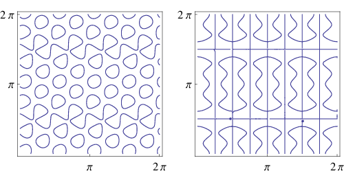
For any two-dimensional surface, it is known [Ch] that the nodal lines are a union of $C^{2}$ -immersed circles, with at most finitely many singular points and the nodal lines through a singular point form an equiangular system, see Figure 1. Thus, with the exception of the singular set, the nodal set of an eigenfunction is rectifiable and we can speak about its length. In the real-analytic case, such as in our case of the flat torus, Donnelly-Fefferman [D-F] showed that the length of the nodal set of an eigenfunction with eigenvalue $E=\lambda^{2}$ is commensurable to $\lambda$ :

(1.3)

\operatorname{length}(\mathcal{N}_{\varphi})\approx\sqrt{E}=\lambda\;.

Refer to caption — Figure 1. Nodal lines for the eigenfunction $\cos(4x-7y)+\sin(8x-y)+\sin(4x+7y)$ (left) and $\sin(4x+7y)+\sin(4x-7y)+\sin(8x+y)+\sin(8x-y)=2\sin 4x\cos y(-1+2\cos 4x+2\cos 2y-2\cos 4y+2\cos 6y)$ (right).

Our goal in this paper is to better understand the local geometry of nodal lines. In this respect, M. Berry argued [Be] that for random plane waves, the nodal lines typically have curvature of order $E$ . If one tries to make a statement for nodal lines of individual eigenfunctions, say in the case of $\mathbb{T}^{2}$ , it is clear that ‘pointwise curvature’ is not the appropriate concept. Indeed, nodal lines (for arbitrary large $E$ ) may have zero curvature or, as is also easily seen, develop arbitrary large pointwise curvature (for a fixed $E$ ).

1.1. The width of nodal lines

In order to formulate an alternative to curvature, we first introduce some terminology.

Definition 1.

An arc $C\subset\mathbb{T}^{2}$ is called ‘regular’ if $C$ admits an arc-length parametrization $\gamma:[0,\ell]\to C$ , $0<\ell<1$ , which is $C^{2}$ and such that for some $\kappa>0$ , the curvature $|\ddot{\gamma}|$ satisfies a pointwise pinching condition

(1.4)

\kappa<|\overset{..}{\gamma}|<2\kappa

and the total curvature is bounded:

(1.5)

2\kappa\ell<1\;.

For a convex curve $C$ the width $w(C)$ is defined as the minimal distance between a pair of parallel supporting lines of the curve (Figure 2).

In the case of regular arcs, we shall see that

(1.6)

w(C)\approx\ell^{2}\kappa

An examination of numerical plots of some nodal sets (see Figure 1) leads one to realize that $\mathcal{N}_{\varphi}$ does not contain “large” curved arcs, specifically that as $E\to\infty$ , for regular arcs $C\subset\mathcal{N}_{\varphi}$ , either their length $\ell\to 0$ shrinks or the curvature pinching $\kappa\to 0$ .

We make the following conjecture:

Conjecture 1.

For all $\varepsilon>0$ , there is $c_{\varepsilon}>0$ such that if $\varphi$ is an eigenfunction of $\mathbb{T}^{2}$ of eigenvalue $E=\lambda^{2}$ and $C$ any regular arc contained in $\mathcal{N}_{\varphi}$ , then

(1.7)

w(C)<c_{\varepsilon}\lambda^{-1+\varepsilon}.

This is our substitute for the phenomenon M. Berry pointed out for random plane waves. The above conjecture seems to be consistent with numerics and we will moreover prove its validity for ‘most’ eigenvalues $E$ .

In generality, we prove

Theorem 1.

If $C\subset\mathcal{N}_{\varphi}$ is a regular arc, then

(1.8)

w(C)<C_{\varepsilon}\lambda^{-\frac{1}{3}+\varepsilon}.

The argument makes crucial use of the structure of lattice points on the circle $\{|\xi|=\lambda\}$ . Relevant results will be presented in § 2.

In § 6 we will show that the exponent $1/3$ of Theorem 1 can be improved to $1/2$ for almost all of the nodal line, in the following sense:

Theorem 2.

Given $\varepsilon>0$ , there is $\delta>0$ such that the following holds. Let $\{C_{\alpha}\}$ be a collection of disjoint regular arcs of $\mathcal{N}_{\varphi}$ satisfying

(1.9)

w(C_{\alpha})>\lambda^{-\frac{1}{2}+\varepsilon}\text{ for each }\alpha.

Then for $\lambda>\lambda(\epsilon)$ ,

(1.10)

\sum_{\alpha}\operatorname{length}(C_{\alpha})<\lambda^{1-\delta}

Recall that $\operatorname{length}(\mathcal{N}_{\varphi})\approx\lambda$ , by (1.3), so that Theorem 2 asserts that arcs of large width form a negligible part of the nodal set.

As we will see, the exponent $\frac{1}{2}$ in (1.9) could be replaced by $1$ , assuming the validity of the Cilleruelo-Granville conjecture [C-G], stating that for all $\varepsilon>0$ , there is a constant $B_{\varepsilon}$ such that any arc on a circle $\{|\xi|=\lambda\}$ of size at most $\lambda^{1-\varepsilon}$ contains at most $B_{\varepsilon}$ lattice points (uniformly in $\lambda$ ).

Finally, we also show that Conjecture 1 holds for at least a positive proportion of the nodal set, in the following sense:

Theorem 3.

There is a constant $c_{0}>0$ such that the following holds. Let $\varepsilon>0$ , $\lambda$ large enough and $\{C_{\alpha}\}$ a collection of disjoint regular arcs of $\mathcal{N}_{\varphi}$ satisfying

(1.11)

w(C_{\alpha})>\lambda^{-1+\varepsilon}\text{ for each }\alpha.

Then

(1.12)

\operatorname{length}(\mathcal{N}_{\varphi}\backslash\bigcup_{\alpha}C_{\alpha})>c_{0}\lambda.

The proofs of Theorems 2 and 3 make essential use of the results of Donnelly and Fefferman [D-F].

1.2. Total curvature

Another geometric characteristic of nodal lines that one can investigate is their total curvature.

For $C^{2}$ curves in $\mathbb{R}^{3}$ , if $\gamma:[0,\ell]\to C$ is a $C^{2}$ arc length parametrization then the total curvature is

(1.13)

K(C)=\int_{0}^{\ell}||\ddot{\gamma}(s)||ds\;.

When one varies the curve $C$ , the formula (1.13) is clearly continuous in the $C^{2}$ topology and hence can be used to define the total curvature of any continuous curve as the limit of the total curvature of its smooth perturbations. However, there is definition of total curvature which makes sense for any continuous curve, which starts with defining the total curvature of a polygon as the sum of the angles subtended by the prolongation of any of its sides and the next one, and then for any continuous curve $C$ setting

(1.14)

K(C)=\sup_{P}K(P)

where the supremum ¹¹ 1 Alternatively one can take (1.15) $K(C)=\lim_{P}K(P)$ where the limit is over all polygons $P$ inscribed in $C$ for which the maximal distance between adjacent vertices tends to zero; this definition works for curves in arbitrary Riemannian manifolds [CL]. is over all polygons $P$ inscribed in $C$ . One can show that for $C^{2}$ curves this definition coincides with (1.13) (see [M]).

We claim that the total curvature $K_{\varphi}$ of the nodal set for an eigenfunction $\varphi$ with eigenvalue $E$ is bounded by

(1.16)

K_{\varphi}\ll E

Note that there is no lower bound, since the nodal set of the eigenfunction $\sin nx$ is a union of non-intersecting lines hence has zero total curvature.

To prove (1.16), it suffices to assume that nodal set is smooth, which is easily seen to be a generic condition in the eigenspace on the torus, hence a small perturbation in the eigenspace will bring us to that setting and one then invokes continuity of the total curvature in the $C^{2}$ -topology. In case the nodal set is smooth, one can make the following comment based on the fact that $\mathcal{N}_{\varphi}$ is a semi-algebraic set. First observe that $\varphi$ in (1.1) may be expressed as

(1.17)

\varphi(x_{1},x_{2})=\sum_{\alpha,\beta}a_{\alpha,\beta}(\cos x_{1})^{\alpha_{1}}(\cos x_{2})^{\alpha_{2}}(\sin x_{1})^{\beta_{1}}(\sin x_{2})^{\beta_{2}}

with $\alpha,\beta\in\mathbb{Z}_{+}^{2}$ and $\alpha_{1}+\alpha_{2}+\beta_{1}+\beta_{2}\leq\sqrt{2}\lambda$ .

Introducing variables $u_{1}=\cos x_{1}$ , $u_{2}=\cos x_{2}$ , it follows that $u_{1},u_{2}$ satisfy a polynomial equation

(1.18)

P(u_{1},u_{2})=0

with $P\in\mathbb{R}[u_{1},u_{2}]$ of degree $d<c\lambda$ . According to [R, Theorem 4.1, Proposition 4.2], assuming $\{P=0\}$ is smooth, its total curvature²² 2 Since the total curvature of an arc is the variation of its tangent vector, a bound is obtained by integration in $s$ of the number of solutions in $u=(u_{1},u_{2})$ of $\begin{cases}\partial_{2}P(u)+s\partial_{1}P(u)=0\\ P(u)=0.\end{cases}$ is at most $const.d^{2}\ll E$ . Since $\mathcal{N}_{\varphi}\subset\{P=0\}$ (in the $u_{1},u_{2}$ -parametrization), we may conclude that (1.16) holds.

1.3. Remarks

(1)

In defining regular arcs, one could make further higher derivative assumptions on the parametrization $\gamma$ (as we will show with an example in Appendix A, those do not hold automatically). Involving higher derivatives would allow to improve upon the estimate (1.8). We do not pursue this direction here however partly because Definition 1 would have to be replaced by a more technical one and it is not clear which version would be the most natural.
(2)

We point out that our estimates for the width are specific to the flat torus. For instance, they are not valid on the sphere $S^{2}$ . Indeed, the standard spherical harmonics $Y_{\ell,m}=P_{\ell,m}(\theta)e^{im\varphi}$ are eigenfunctions for which the circles of latitude $\{P_{\ell,m}(\theta)=0\}$ are families of regular arcs with geodesic curvature bounded away from zero.
(3)

One can easily obtain the analogue of (1.16) for the total curvature of the nodal sets on the sphere using similar arguments to those on the torus. At the time of this writing, it is not clear to us if there is an estimate of the type (1.16) for general real-analytic surfaces, or even, more modestly, any explicit bound $K_{\varphi}<K(E)$ for the total curvature.

Acknowledgements: We thank Misha Sodin for his comments. J.B. was supported in part by N.S.F. grant DMS 0808042. Z.R. was supported by the Oswald Veblen Fund during his stay at the Institute for Advanced Study and by the Israel Science Foundation (grant No. 1083/10).

2. Lattice points on circles

In this section, we collect some facts about lattice points on arcs for later use. Let $E=\lambda^{2}\in\mathbb{Z}_{+}$ and

\mathcal{E}=\mathbb{Z}^{2}\cap\{|x|=\lambda\}

Then $|\mathcal{E}|=r_{2}(E)$ is the number of representations of $E$ as a sum of two squares, which is essentially the number of divisors of $E$ in the ring of Gaussian integers. In particular one has an upper bound

(2.1)

r_{2}(E)\ll\exp c\frac{\log E}{\log\log E}\ll E^{\varepsilon}\text{ for all }\varepsilon>0\;.

The next statement is a slight specification of a more general result due to Jarnik [J].

Lemma 1.

Let $P_{0},P_{1},P_{2}\in\mathcal{E}$ be distinct and $|P_{0}-P_{1}|\leq|P_{0}-P_{2}|$ . Then

(2.2)

|P_{0}-P_{2}|^{2}.|P_{0}-P_{1}|>c\lambda

(here and in the sequel, $c,C$ will denote constants).

Proof.

$P_{0},P_{1},P_{2}$ belong to an arc $C\subset\{|x|=\lambda\}$ of size $r$ and we may obviously assume $r<\sqrt{\lambda}$ . Since $P_{0},P_{1},P_{2}$ are distinct, they span a triangle $T$ of area

0<\operatorname{area}(T)=\frac{1}{2}\Big|\det\begin{pmatrix}1&P_{0}\\ 1&P_{1}\\ 1&P_{2}\end{pmatrix}\Big|\in\frac{1}{2}\mathbb{Z}_{+}.

Hence, from geometric considerations

\frac{1}{2}\leq\text{ area }(T)<c\frac{r^{2}}{\lambda}.|P_{0}-P_{1}|

∎

Lemma 2.

Let $P_{0},P_{1},Q_{0},Q_{1}\in\mathcal{E}$ be distinct points on an arc of size $r$ . Then

(2.3)

|P_{0}-Q_{0}|.|P_{1}-Q_{1}|.r>c\lambda.

Proof.

We may assume $r<\frac{1}{100}\lambda$ . For $\alpha=0,1$ , let

	$\displaystyle P_{\alpha}$	$\displaystyle=\lambda e^{i\theta_{\alpha}}$
	$\displaystyle P_{\alpha}-Q_{\alpha}$	$\displaystyle=\Delta_{\alpha}e^{i\psi_{\alpha}}.$

Then (possibly permuting $P_{\alpha},Q_{\alpha}$ )

\Delta^{2}_{\alpha}=|P_{\alpha}-Q_{\alpha}|^{2}=2P_{\alpha}.(P_{\alpha}-Q_{\alpha})=2\lambda\Delta_{\alpha}\cos(\theta_{\alpha}-\psi_{\alpha})\sim 2\lambda\Delta_{\alpha}\Big(\frac{\pi}{2}+\theta_{\alpha}-\psi_{\alpha}\Big)

implying that

(2.4)		$\displaystyle\psi_{\alpha}$	$\displaystyle=\frac{\pi}{2}+\theta_{\alpha}+0\Big(\frac{\Delta_{\alpha}}{\lambda}\Big)$
(2.4)		$\displaystyle\|\psi_{0}-\psi_{1}\|$	$\displaystyle=\|\theta_{0}-\theta_{1}\|+0\Big(\frac{\Delta_{0}+\Delta_{1}}{\lambda}\Big)$

Since the vectors $P_{0}-Q_{0},P_{1}-Q_{1}$ are not parallel,

|\det(P_{0}-Q_{0},P_{1}-Q_{1})|\geq 1

and thus

(2.5)

\Delta_{0}.\Delta_{1}.|\psi_{0}-\psi_{1}|\geq 1

From (2.4) (2.5)

1\leq\Delta_{0}\Delta_{1}|\theta_{0}-\theta_{1}|+0\big(\lambda^{-1}\Delta_{0}\Delta_{1}(\Delta_{0}+\Delta_{1})\big)

and

\lambda<2\Delta_{0}\Delta_{1}|P_{0}-P_{1}|+0\big(\Delta_{0}\Delta_{1}(\Delta_{0}+\Delta_{1})\big)<Cr\Delta_{0}\Delta_{1}\;.

∎

Let us also recall the results from Cilleruelo-Cordoba[C-C] and Cilleruelo-Granville [C-G] on the spacing properties of systems $\{P_{1},\ldots,P_{m}\}$ of distinct elements of $\mathcal{E}$ .

Lemma 3.

([C-C], [C-G])

\prod_{1\leq i<j\leq m}|P_{i}-P_{j}|\geq\begin{cases}\lambda^{\frac{m}{2}(\frac{m}{2}-1)}\text{ if $m$ is even}\\ \lambda^{\frac{1}{4}(m-1)^{2}}\text{ if $m$ is odd.}\end{cases}

The argument in [C-C] is arithmetic and based on factorization of $E=\lambda^{2}$ in Gaussian primes. The following elegant and much simpler argument was given by Ramana [Ra]: We identify the standard lattice $\mathbb{Z}^{2}\subset\mathbb{R}^{2}$ with the Gaussian integers $\mathbb{Z}[\sqrt{-1}]\subset\mathbb{C}$ . If $\overline{P}$ denotes the complex conjugate of $P$ , then our condition on the lattice points being on one circle says that

(2.6)

P_{j}\overline{P_{j}}=\lambda^{2},\quad j=1,\dots,m

Ramana observed that for any $0\leq k\leq m-1$ , we have an identity

(2.7)

\lambda^{k(k+1)}\prod_{1\leq i<j\leq m}(P_{i}-P_{j})=\prod_{i=1}^{m}P_{i}^{k}\cdot\det V_{k,m}

where $V_{k,m}$ is the following Vandermonde type matrix

(2.8)

V_{k,m}=\begin{pmatrix}\overline{P_{1}}^{k}&\overline{P_{2}}^{k}&\dots&\overline{P_{m}}^{k}\\ \overline{P_{1}}^{k-1}&\overline{P_{2}}^{k-1}&\dots&\overline{P_{m}}^{k-1}\\ \vdots\\ 1&1&\dots&1\\ P_{1}&P_{2}&\dots&P_{m}\\ \vdots\\ P_{1}^{m-1-k}&P_{2}^{m-1-k}&\dots&P_{m}^{m-1-k}\\ \end{pmatrix}

To see this, we compute the RHS of (2.7) by noting that $P_{i}^{k}\det V_{k,m}$ is the determinant of the matrix resulting from multiplying the $i$ -th column of $V_{k,m}$ by $P_{i}^{k}$ , and using (2.6) one is reduced to computing an ordinary Vandermonde determinant, yielding the LHS of (2.7).

Once (2.7) is established, we take absolute values and noting that $|\det V_{k,m}|^{2}\geq 1$ since it is a nonzero integer , we get

(2.9)

\lambda^{k(k+1)}\prod_{1\leq i<j\leq m}|P_{i}-P_{j}|\geq\lambda^{km}

Taking $k=\lfloor\frac{m}{2}\rfloor$ gives Lemma 3. ∎

Taking $m=2$ in Lemma 3, it follows that

|P_{0}-P_{1}|\ |P_{1}-P_{2}|\ |P_{2}-P_{0}|\geq\lambda

and we are recovering (2.2).

Lemma 3 implies a uniform bound $B(\varepsilon)$ on the number of elements of $\mathcal{E}$ on an arc $C\subset\{|x|=\lambda\}$ of size $r<\lambda^{\frac{1}{2}-\varepsilon}$ . More precisely

Lemma 4 ([C-C]).

Let $\delta(m)=\frac{1}{4\lfloor\frac{m}{2}\rfloor+2}$ . If $C\subset\{|x|=\lambda\}$ is an arc of length $r<\sqrt{2}\lambda^{\frac{1}{2}-\delta(m)}$ , then $\#\mathcal{E}\cap C\leq m$ .

Cilleruello and Granville conjectured a uniform bound on the number of lattice points on any arc of length $\lambda^{1-\epsilon}$ :

Conjecture 2.

[C-G, Conjecture 14] Let $0<\epsilon<1$ . Then there is some $B_{\epsilon}>0$ so that the number of lattice points on any arc $C\subset\{|x|=\lambda\}$ of length $r<\lambda^{1-\epsilon}$ is at most $B_{\epsilon}$ .

Conjecture 2 is true for most $E=\lambda^{2}\in\mathbb{Z}_{+}$ , in fact we have the stronger statement that all lattice points on the circle of radius $\sqrt{E}$ are well separated. To make sense of it, recall that the number of $E\leq N$ which are a sum of two squares is asymptotic to a constant multiple of $N/\sqrt{\log N}$

Lemma 5.

Fix $\epsilon>0$ . Then for all but $O(N^{1-\epsilon/3})$ integers $E\leq N$ , one has

(2.10)

\min_{\begin{subarray}{c}x\neq y\in\mathbb{Z}^{2}\\ |x|^{2}=|y|^{2}=E\end{subarray}}|x-y|>(\sqrt{E})^{1-\epsilon}

Proof.

We will say that $E\leq N$ is “exceptional” if there is a pair of close points $|x|^{2}=|y|^{2}=E$ , $0<|x-y|<\sqrt{E}^{1-\epsilon}$ . Writing $z=x-y$ , we see that the number of exceptional $E$ ’s is bounded by the number of pairs of integer vectors $x\in\mathbb{Z}^{2}$ , $0\neq z\in\mathbb{Z}^{2}$ with

(2.11)

|x|^{2}\leq N,\quad 0<|z|<\sqrt{E}^{1-\epsilon}

and satisfying

(2.12)

2x\cdot z=|z|^{2}

Writing $z=dz^{\prime}$ with $d\geq 1$ and $z^{\prime}\in\mathbb{Z}^{2}$ primitive, we see that the number of $x<\sqrt{N}$ lying on the line (2.12) is $O(\sqrt{N}/|z^{\prime}|)$ and hence the number of exceptional $E\leq N$ is dominated by

(2.13)

\sum_{1\leq d\leq\sqrt{N}^{1-\epsilon}}\sum_{\begin{subarray}{c}z^{\prime}\in\mathbb{Z}^{2}\mbox{ primitive}\\ |z^{\prime}|\leq(\sqrt{N})^{1-\epsilon}/d\end{subarray}}\frac{\sqrt{N}}{|z^{\prime}|}\ll\sqrt{N}\sum_{1\leq d\leq\sqrt{N}^{1-\epsilon}}\frac{(\sqrt{N})^{1-\epsilon}}{d}\ll N^{1-\epsilon/2}\log N

which proves our claim. ∎

3. The width of a regular arc

Recall that the width of a convex curve $C$ is defined as the minimal distance between a pair of parallel supporting lines of the curve. We denote it by $w(C)$ .

Lemma 6.

Let $C$ be a regular arc, that is admitting an arc length parametrization $\gamma:[0,\ell]\to C$ with curvature pinched by $\kappa<|\ddot{\gamma}|<2\kappa$ and with total curvature bounded by $2\kappa\ell<1$ . Then the width of $C$ is commensurate with

(3.1)

w(C)\approx\ell^{2}\kappa

Proof.

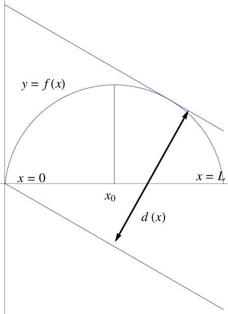
We may present $C$ as the graph of a function $f$ :

C=\{(x,f(x)):0<x<L\}

where $f(x)\geq 0$ , and $f(0)=0=f(L)$ (see Figure 3).

Note that our assumptions in particular imply that the arc is convex, since there are no inflection points (the curvature is nowhere zero) and the total curvature is small. Hence $f^{\prime\prime}<0$ , and the function $f$ has a unique critical point at $x_{0}\in(0,L)$ where $f$ is maximal.

We now note that the assumption of total curvature being at most $1$ implies a bound for the derivative of $f$ :

|f^{\prime}(x)|<2

Indeed, $f^{\prime}(x)=\tan\theta(x)$ where $\theta(x)$ is the angle between the tangent vector to the arc at $(x,f(x))$ and the $x$ -axis. At the point $x_{0}$ we have $\theta(x_{0})=0$ and the total variation of $\theta$ is just the total curvature which is at most $1$ . Hence $|f^{\prime}(\theta)|\leq\tan 1<2$ .

The curvature at the point $(x,f(x))$ is

\kappa(x)=\frac{|f^{\prime\prime}(x)|}{(1+f^{\prime}(x)^{2})^{3/2}}

Since $|f^{\prime}|<1$ , the second derivative $f^{\prime\prime}$ and the curvature $\kappa(x)$ are commensurable and so $|f^{\prime\prime}(x)|$ is commensurate with $\kappa$ :

(3.2)

|f^{\prime\prime}(x)|\approx\kappa

We claim that the width of $C$ is the value of $f$ at the critical point $x_{0}$ :

(3.3)

w(C)=f(x_{0})

To see this, note that the supporting line $L_{1}(t)$ of $C$ at the point $(t,f(t))$ for $0<t<L$ is the tangent line

L_{1}(t):y=f^{\prime}(t)x+f(t)-tf^{\prime}(t)

At $t=x_{0}$ this is the line $y=f(x_{0})$ and the other supporting line $L_{2}(x_{0})$ of $C$ parallel to it is the $x$ -axis $y=0$ , and $f(x_{0})$ is the distance between these two lines. For $0<t<x_{0}$ the other supporting line $L_{2}(t)$ parallel to $L_{1}(t)$ goes through the end point $(L,0)$ of the arc, with equation

L_{2}(t):y=f^{\prime}(t)(x-L),\qquad 0<t<x_{0}

while for $x_{0}<t<L$ , the line $L_{2}(t)$ passes through the origin $(0,0)$ with equation

L_{2}(t):y=f^{\prime}(t)x,\qquad x_{0}<t<L

Hence the distance between $L_{1}(t)$ and $L_{2}(t)$ is

(3.4)

d(t)=\frac{g(t)}{\sqrt{1+f^{\prime}(t)^{2}}},\quad g(t)=\begin{cases}f(t)+(L-t)f^{\prime}(t),&0<t<x_{0}\\ f(t)-tf^{\prime}(t),&x_{0}<t<L\end{cases}

Since $|f^{\prime}(t)|<2$ , this shows that

(3.5)

d(t)\approx g(t)

and it suffices to show that

g(t)\geq g(x_{0})=f(x_{0})

If $0<t<x_{0}$ then $g^{\prime}(t)=(L-t)f^{\prime\prime}(t)<0$ so $g$ is decreasing and so $g(t)>g(x_{0})=f(x_{0})$ , while if $x_{0}<t<L$ then $g^{\prime}(t)=-tf^{\prime\prime}(t)>0$ so $g$ is increasing and so $g(t)>g(x_{0})=f(x_{0})$ .

Having established that $w(C)\approx f(x_{0})$ , it remains to show that

f(x_{0})\approx\kappa\ell^{2}

Assuming say that $x_{0}\leq L/2$ , we expand $f$ in a Taylor series around the endpoint $x=L$ further from $x_{0}$ , finding

(3.6)

0=f(L)=f(x_{0})+f^{\prime}(x_{0})(L-x_{0})+\frac{1}{2}f^{\prime\prime}(y)(L-x_{0})^{2}

for some $x_{0}<y<L$ . Using $f(L)=0$ , $f^{\prime}(x_{0})=0$ and $f^{\prime\prime}<0$ , $|f^{\prime\prime}|\approx\kappa$ and $L/2\leq L-x_{0}\leq L$ we get

f(x_{0})=-\frac{1}{2}f^{\prime\prime}(y)(L-x_{0})^{2}\approx\kappa L^{2}

Now note that $L\approx\ell$ because

\ell=\int_{0}^{L}\sqrt{1+f^{\prime}(t)^{2}}dt\in[L,3L]

using $|f^{\prime}(x)|<2$ . Hence $f(x_{0})\approx\kappa\ell^{2}$ as claimed. ∎

4. Local estimates on the width

4.1. Fourier transforms of arcs

We establish some bounds on the Fourier transform of measures supported by “regular” arcs.

Let $\gamma:[0,\ell]\to C$ be an arc-length parameterization of the regular arc $C$ , so that $|\dot{\gamma}|=1$ , and $\kappa<|\overset{..}{\gamma}|<2\kappa$ . Note that if $\xi\in\mathbb{R}^{2},|\xi|=1$ and $0<\rho<\frac{\ell\kappa}{10}$ , then

(4.1)

I_{\xi}=\{t\in I:|\xi\cdot\dot{\gamma}(t)|<\rho\}

is an interval of size at most $O(\rho/\kappa)$ .

Indeed, the length of $I_{\xi}$ can be computed as

(4.2)

\int_{I_{\xi}}dt=\int_{|u|<\rho}\frac{du}{|\xi\cdot\ddot{\gamma}(t)|}

one using the change of variable $u=\xi\cdot\dot{\gamma}(t)$ . Denoting by $\theta(t)$ the angle between $\xi$ and the unit tangent $\dot{\gamma}(t)$ to the curve, so that by assumption $|\cos\theta(t)|=|\xi\cdot\dot{\gamma}(t)|<\rho$ , we have on noting that $\ddot{\gamma}$ is the normal vector to the curve, that

(4.3)

|\xi\cdot\ddot{\gamma}(t)|=|\ddot{\gamma}(t)||\sin\theta(t)|>\kappa\sqrt{1-\rho^{2}}

and hence

(4.4)

\operatorname{length}I_{\xi}<\frac{2\rho}{\kappa\sqrt{1-\rho^{2}}}\ll\frac{\rho}{\kappa}

since $\rho<\ell\kappa/10<1/10$ .

Lemma 7.

Let $\xi\in\mathbb{R}^{2}\backslash\{0\}$ and assume

(4.5)

\Big|\frac{\xi}{|\xi|}\cdot\dot{\gamma}(t)\Big|>\rho\text{ for all }t\in[0,\ell]\;.

Let $\omega:\mathbb{R}\to\mathbb{R}_{+}$ , $\operatorname{supp}\omega\subset[0,\ell]$ satisfy

(4.6)

\int\omega=1\text{ and }\int|\omega^{\prime}|<\frac{c}{\ell}\;.

Then

(4.7)

\Big|\int e\big(\xi\cdot\gamma(t)\big)\omega(t)dt\Big|<\frac{c}{\rho|\xi|}\Big(\frac{1}{\ell}+\frac{\kappa}{\rho}\Big)

(where $c$ denotes various constants).

Proof.

A change of variables $u=\xi\cdot\gamma(t)$ gives

		$\displaystyle\Big\|\int e\big(\xi\cdot\gamma(t)\big)\omega(t)dt\Big\|\leq\int\Big\|\frac{d}{dt}\Big[\frac{\omega(t)}{\xi\cdot\dot{\gamma}(t)}\Big]\Big\|dt\leq\int\Big\{\frac{\|\dot{\omega}(t)\|}{\|\xi\cdot\dot{\gamma}(t)\|}+\frac{\omega(t)\|\xi\cdot\overset{..}{\gamma}(t)\|}{\|\xi\cdot\dot{\gamma}(t)\|^{2}}\Big\}$
		$\displaystyle\leq\frac{1}{\rho\|\xi\|}\int\|\dot{\omega}(t)\|+\frac{\kappa}{\rho^{2}\|\xi\|}\int\omega(t)<\frac{c}{\rho\ell\|\xi\|}+\frac{\kappa}{\rho^{2}\|\xi\|}$

from the assumptions. ∎

Fix $E\in\mathbb{Z}_{+}$ (large), $\lambda=\sqrt{E}$ and let $\mathcal{E}=\mathbb{Z}^{2}\cap\{|x|=\lambda\}$ . Fix $0<c_{0}<\frac{1}{100}$ and take $\rho=c_{0}\kappa\ell/|\mathcal{E}|^{2}$ . We let $\xi$ run over all vectors $\xi=\frac{\xi_{1}-\xi_{2}}{|\xi_{1}-\xi_{2}|}$ , $\xi_{1}\not=\xi_{2}$ in $\mathcal{E}$ . Excluding the corresponding subintervals $I_{\xi}$ of (4.1) from $I$ , of length $|I_{\xi}|<c_{0}\ell|\mathcal{E}|^{-2}$ , we obtain

Lemma 8.

There is a collection of at most $|\mathcal{E}|^{2}$ disjoint sub-intervals $I_{\tau}\subset I$ with the following properties:

(4.8)

|I_{\tau}|>c_{0}|\mathcal{E}|^{-2}\ell

(4.9)

\sum|I_{\tau}|>(1-2c_{0})\ell

(4.10)

\Big|\dot{\gamma}(t)\cdot\frac{\xi_{1}-\xi_{2}}{|\xi_{1}-\xi_{2}|}\Big|>c_{0}\frac{\kappa\ell}{|\mathcal{E}|^{2}}\quad\text{ for }\xi_{1}\not=\xi_{2}\text{ in $\mathcal{E}$ and $t\in I$}

Let $\omega:\mathbb{R}\to\mathbb{R}_{+}$ , $\operatorname{supp}\omega\subset I_{\tau}$ satisfy

(4.11)

\int\omega=1\text{ and }\int|\dot{\omega}|\lesssim\frac{|\mathcal{E}|^{2}}{c_{0}\ell}\;.

Then for all $\xi_{1}\not=\xi_{2}$ in $\mathcal{E}$

(4.12)

\Big|\int e\big((\xi_{1}-\xi_{2})\cdot\gamma(t)\big)\omega(t)dt\Big|\lesssim\frac{|\mathcal{E}|^{4}}{c_{0}^{2}\omega(C)}\ \frac{1}{|\xi_{1}-\xi_{2}|}

where $\omega(C)=\ell^{2}\kappa$ is the width of $C$ .

The estimate (4.12) follows indeed from (4.7) and the above choice of $\rho$ .

Returning to Theorem 1, we simply replace $I$ by some $I_{\tau}$ and $C$ by $C_{\tau}=\gamma(I_{\tau})$ . Redefining $\ell=|I_{\tau}|$ , we have for all $\xi_{1}\not=\xi_{2}\in\mathcal{E}$ the estimate

(4.13)

\Big|\int e\big((\xi_{1}-\xi_{2})\cdot\gamma(t)\big)\omega(t)dt\Big|\ll\frac{\lambda^{\varepsilon}}{\omega(C)|\xi_{1}-\xi_{2}|}

if $\omega:\mathbb{R}\to\mathbb{R}_{+}$ , $\operatorname{supp}\omega\subset I$ satisfies

(4.14)

\int\omega=1,\quad\int|\dot{\omega}|\lesssim\frac{1}{\ell}\;.

4.2. The exponent $1/6$

As a warm-up, we show how to prove Conjecture 1 for almost all energies $E$ and how to obtain a weaker version of Theorem 1 with the exponent $1/6$ instead of $1/3$ .

Consider the Fourier expansion of $\varphi$ :

(4.15)

\varphi(x)=\sum_{\xi\in\mathcal{E}}\widehat{\varphi}(\xi)e(x\cdot\xi).

Since the Fourier coefficients of $\varphi$ satisfy $\sum_{\xi\in\mathcal{E}}|\widehat{\varphi}(\xi)|^{2}=||\varphi||_{2}^{2}$ , we have $|\widehat{\varphi}(\xi)|\leq||\varphi||_{2}$ for all $\xi\in\mathcal{E}$ and hence there is some $\xi_{0}$ for which

|\widehat{\varphi}(\xi_{0})|\geq\frac{||\varphi||_{2}}{\sqrt{|\mathcal{E}|}}

Replacing $\varphi$ by $\varphi/\widehat{\varphi}(\xi_{0})$ , we may thus assume

(4.16)

\widehat{\varphi}(\xi_{0})=1,\quad||\varphi||_{2}\leq\sqrt{|\mathcal{E}|}

and in particular $|\widehat{\varphi}(\xi)|\ll\lambda^{\epsilon}$ for all $\epsilon>0$ .

Assume $C\subset\mathcal{N}_{\varphi}$ . Since $\varphi\big(\gamma(t)\big)=0$ , we obtain for any weight function $\omega$ as in Lemma 7 that

(4.17)

\begin{split}0&=\int_{I}\varphi\big(\gamma(t)\big)e\big(-\xi_{0}\cdot\gamma(t)\big)\omega(t)dt\\ &=1+\sum_{\xi\neq\xi_{0}}\widehat{\varphi}(\xi)\int_{I}e\big((\xi-\xi_{0})\cdot\gamma(t)\big)\omega(t)dt\end{split}

By Jarnik, there is at most one frequency $\xi_{1}\neq\xi_{0}$ at distance $\ll\lambda^{1/3}$ from $\xi_{0}$ . For all other frequencies we use (4.12) together with $\sum_{\xi}|\widehat{\varphi}(\xi)|^{2}\leq|\mathcal{E}|\ll\lambda^{\epsilon}$ to get

(4.18)

1+\widehat{\varphi}(\xi_{1})\int e\big((\xi_{1}-\xi_{0})\cdot\gamma(t)\big)\omega(t)dt\ll\frac{\lambda^{\epsilon}}{w}\sum_{\xi\neq\xi_{0},\xi_{1}}\frac{|\widehat{\varphi}(\xi)|}{|\xi-\xi_{0}|}\ll\frac{\lambda^{-1/3+\epsilon}}{w}

We may now show that Conjecture 1 holds for almost all $E$ . First choose $E=\lambda^{2}$ satisfying (2.10). Then $\xi_{1}$ does not exist and $|\xi-\xi_{0}|>\lambda^{1-\epsilon}$ for $\xi\neq\xi_{0}$ , hence (4.18) gives $1\ll\lambda^{-1+\epsilon}/w$ , that is $w\ll\lambda^{-1+\epsilon}$ .

Returning to the case of general $E$ , if there is no such $\xi_{1}$ , that is if $\xi_{0}$ is at distance at least $\lambda^{1/3}$ from all other frequencies, then (4.18) implies $w\ll\lambda^{-1/3+\epsilon}$ .

Otherwise, that is if there is a neighbour $\xi_{1}$ , we proceed as follows: Start by performing a rotation $T$ of the plane as to insure

(4.19)

T(\xi_{1}-\xi_{0})=(|\xi_{1}-\xi_{0}|,0)\in\mathbb{R}^{2}.

Denoting $T\gamma$ again by $\gamma=(\gamma_{1},\gamma_{2})$ , we obtain from (4.18) that

(4.20)

1+\widehat{\varphi}(\xi_{1})\int e\big((|\xi_{1}-\xi_{0}|\gamma_{1}(t)\big)\omega(t)dt\ll\frac{\lambda^{-1/3+\epsilon}}{w}

Next we specify $\omega$ . Writing $\dot{\gamma}(s)=e^{i\theta(s)}$ , we have $\dot{\theta}(s)\sim\kappa$ (or $-\kappa$ , which is similar) and

\overset{..}{\gamma}_{1}(s)=-\big(\sin\theta(s)\big)\dot{\theta}(s)\sim-\sqrt{1-\dot{\gamma}_{1}(s)^{2}}\kappa.

Therefore there is a suitable restriction of $s\in I_{1}\subset I$ , $|I_{1}|\sim\ell$ and some $\rho\gtrsim\kappa\ell$ (recall that $\kappa\ell<1$ ) such that

(4.21)

|\dot{\gamma}_{1}(s)-\rho|<c\kappa\ell<\frac{\rho}{10}\text{ for }s\in I_{1}.

Let $s_{0}\in I_{1}$ be the center of $I_{1}$ . Define

(4.22)

\omega(s)=\frac{\dot{\gamma}_{1}(s)\eta\big(\gamma_{1}(s)-\gamma_{1}(s_{0})\big)}{\int_{I_{1}}\dot{\gamma}_{1}(s)\eta\big(\gamma_{1}(s)-\gamma_{1}(s_{0})\big)ds}

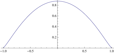
where $\eta$ is a bump-function of the form $\eta(x)=\eta_{0}(\frac{x}{\rho\ell})$ with $\eta_{0}\geq 0$ , $\int\eta_{0}=1$ (see Figure 4),

chosen as to ensure that $\operatorname{supp}\omega\subset I_{1}$ (we use (4.21) here). Also

0\leq\omega<\frac{c}{\ell},\quad\int\omega=1

and

\int|\omega^{\prime}|\lesssim\frac{\kappa}{\rho}+\frac{1}{\ell}\lesssim\frac{1}{\ell}

and (4.14) holds.

With the choice (4.22) and change of variable $u=\gamma_{1}(s)-\gamma_{1}(s_{0})$ , one obtains in (4.38)

(4.23)

\begin{split}\int e\big(|\xi_{1}-\xi_{0}|\gamma_{1}(t)\big)\omega(t)dt&=e\big(|\xi_{1}-\xi_{0}|\gamma_{1}(s_{0})\big)\frac{\int e(|\xi_{1}-\xi_{0}|u)\eta(u)du}{\int\eta(u)du}\\ &=e\big(|\xi_{1}-\xi_{0}|\gamma_{1}(s_{0})\big)\frac{1}{\rho\ell}\int e(|\xi_{1}-\xi_{0}|u)\eta(u)du\\ &=e\big(|\xi_{1}-\xi_{0}|\gamma_{1}(s_{0})\big)\int e(\rho\ell|\xi_{1}-\xi_{0}|t)\eta_{0}(t)dt\end{split}

since $\eta_{0}(t)=\eta(\rho\ell t)$ . Thus we find

(4.24)

1+e\big(|\xi_{1}-\xi_{0}|\gamma_{1}(s_{0})\big)b\ll\frac{\lambda^{-1/3+\epsilon}}{w}

where

(4.25)

b=\widehat{\eta}_{0}(|\xi_{1}-\xi_{0}|\rho\ell)\widehat{\varphi}(\xi_{1})

satisfies $|b|\ll\lambda^{\epsilon}$ .

Note that our choice of $s_{0}\in I_{1}$ allows moving $s_{0}$ within an interval $I_{2}\subset I_{1}$ of size $|I_{2}|=\frac{1}{2}|I_{1}|\sim\ell$ . Since $\gamma_{1}(I_{2})$ contains an interval of size at least $\sim\rho\ell\gtrsim w$ , it follows that

(4.26)

\max_{s_{0}\in I_{2}}\Big|1+be\big(|\xi_{1}-\xi_{0}|\gamma_{1}(s_{0})\big)\Big|\geq\max_{u\in U}\Big|1+be(u)\Big|

where $U\subset\mathbb{R}$ is some interval of size $\sim|\xi_{1}-\xi_{0}|w$ . Then we have

(4.27)

\eqref{3.34'}\geq\frac{1}{2}\min(1,w|\xi_{1}-\xi_{0}|)

Indeed, if $|b|\geq 3/2$ or $|b|\leq 1/2$ then $|1+be(u)|\geq 1/2$ , while if $1/2<|b|<3/2$ then we can bound

\max_{u\in U}|1+be(u)|\geq|b|\max_{u\in U}|\sin u|\geq\frac{1}{4}|U|

Thus we find

(4.28)

\min(1,w|\xi_{1}-\xi_{0}|)\ll\frac{\lambda^{-1/3+\epsilon}}{w}

If the minimum is $1$ , we get $w\ll\lambda^{-1/3+\epsilon}$ . Otherwise (taking into account $|\xi_{1}-\xi_{0}|\geq 1$ ) we get

w\ll\lambda^{-1/6+\epsilon}

4.3. Proof of Theorem 1

Fix some $\xi_{0}\in\mathcal{E}$ and enumerate $\mathcal{E}=\xi_{0},\xi_{1},\ldots$ such that

(4.29)

|\xi_{0}-\xi_{j}|\leq|\xi_{0}-\xi_{j+1}|.

Write

(4.30)

\varphi(x)=\sum_{j}c_{j}e(x\cdot\xi_{j}).

Let $1<r<\frac{1}{10}\lambda$ be a parameter and take $J\in\mathbb{Z}_{+}$ with

(4.31)

|\xi_{0}-\xi_{J}|\leq r,\quad|\xi_{0}-\xi_{J+1}|\geq r\;.

Assume $C\subset\mathcal{N}_{\varphi}$ . Then since $\varphi\big(\gamma(t)\big)=0$ , we obtain for any weight function $\omega$ as in Lemma 7 that

(4.32)		$\displaystyle 0$	$\displaystyle=\int\varphi\big(\gamma(t)\big)e\big(-\xi_{0}\cdot\gamma(t)\big)\omega(t)dt$
(4.32)			$\displaystyle=c_{0}+\sum_{1\leq j\leq J}c_{j}\int e\big((\xi_{j}-\xi_{0})\cdot\gamma(t)\big)\omega(t)dt$

(4.33)

+0\Big(\frac{\lambda^{\varepsilon}}{w}\sum_{j>J}\frac{|c_{j}|}{|\xi_{0}-\xi_{j}|}\Big)

Perform a rotation $T$ of the plane as to insure

(4.34)

T(\xi_{J}-\xi_{0})=(\xi^{\prime}_{J},0),\quad\xi^{\prime}_{J}=|\xi_{J}-\xi_{0}|

and denote

(4.35)

T(\xi_{j}-\xi_{0})=(\xi_{j}^{\prime},\zeta_{j}^{\prime})\in\mathbb{R}^{2}.

Clearly

(4.36)

\xi_{j}^{\prime}\sim|\xi_{j}-\xi_{0}|,\quad j\leq J

and

(4.37)

|\zeta_{j}^{\prime}|<2\frac{r}{\lambda}|\xi_{j}-\xi_{0}|.

Denoting $T\gamma$ again by $\gamma=(\gamma_{1},\gamma_{2})$ , we easily obtain

(4.38)		(4.32)	$\displaystyle=$	$\displaystyle c_{0}+\sum_{1\leq j\leq J}\Big[\int e\big(\xi_{j}^{\prime}\gamma_{1}(t)\big)\omega(t)dt\Big]c_{j}$
(4.39)			$\displaystyle+$	$\displaystyle 0\Big(\frac{r}{\lambda}\sum_{0<j<J}\|c_{j}\|\ \|\xi_{j}-\xi_{0}\|\Big).$

Next we specify $\omega$ as in § 4.2, by picking a subinterval $I_{1}\subset I$ $|I_{1}|\approx\ell$ , such that

(4.40)

|\dot{\gamma}_{1}(s)-\rho|<c\kappa\ell<\frac{\rho}{10}\text{ for }s\in I_{1}.

for some $\rho\gtrsim\kappa\ell$ (recall that $\kappa\ell<1$ ). Let $s_{0}\in I_{1}$ be the center of $I_{1}$ . Define

(4.41)

\omega(s)=\frac{\dot{\gamma}_{1}(s)\eta\big(\gamma_{1}(s)-\gamma_{1}(s_{0})\big)}{\int_{I_{1}}\dot{\gamma}_{1}(s)\eta\big(\gamma_{1}(s)-\gamma_{1}(s_{0})\big)ds}

where $\eta$ is a bump-function of the form $\eta(x)=\eta_{0}(\frac{x}{\rho\ell})$ with $\eta_{0}\geq 0$ , $\int\eta_{0}=1$ , chosen as to ensure that $\operatorname{supp}\omega\subset I_{1}$ (we use (4.40) here). Also

0\leq\omega<\frac{c}{\ell},\quad\int\omega=1

and

\int|\omega^{\prime}|\lesssim\frac{\kappa}{\rho}+\frac{1}{\ell}\lesssim\frac{1}{\ell}

and (4.14) holds.

With the choice (4.41) and change of variable $u=\gamma_{1}(s)-\gamma_{1}(s_{0})$ , one obtains in (4.38)

(4.42)

\begin{split}\int e\big(\xi_{j}^{\prime}\gamma_{1}(t)\big)\omega(t)dt&=e\big(\xi_{j}^{\prime}\gamma_{1}(s_{0})\big)\frac{\int e(\xi_{j}^{\prime}u)\eta(u)du}{\int\eta(u)du}\\ &=e\big(\xi_{j}^{\prime}\gamma_{1}(s_{0})\big)\frac{1}{\rho\ell}\int e(\xi_{j}^{\prime}u)\eta(u)du\\ &=e\big(\xi_{j}^{\prime}\gamma_{1}(s_{0})\big)\int e(\rho\ell\xi_{j}^{\prime}t)\eta_{0}(t)dt\end{split}

since $\eta_{0}(t)=\eta(\rho\ell t)$ .

Therefore

|\eqref{3.27}|<\lambda^{-100}\text{ unless }|\xi_{j}^{\prime}|<\frac{\lambda^{\varepsilon}}{\rho\ell}.

Hence, in (4.38)

(4.43)

\Big|\int e\big(\xi_{j}^{\prime}\gamma_{1}(t)\big)\omega(t)dt\Big|<\lambda^{-100}\text{ unless }|\xi_{j}^{\prime}|<\frac{\lambda^{\varepsilon}}{w(C)}

and from (4.32), (4.33)

(4.44)

\Big|c_{0}+\sum_{0<|\xi_{j}-\xi_{0}|<\frac{\lambda^{\varepsilon}}{w}}c_{j}^{\prime}\Big[\int e(\rho\ell\xi_{j}^{\prime}t)\varphi_{0}(t)dt\Big]\Big|<\eqref{3.18}+\eqref{3.24}+\lambda^{-\frac{1}{100}}

where

(4.45)

c_{j}^{\prime}=e\big(\xi_{j}^{\prime}\gamma_{1}(s_{0})\big)c_{j}.

Arguing by contradiction, assume

(4.46)

w(C)>\lambda^{-\frac{1}{3}+5\varepsilon}\;.

Since $|\xi_{2}-\xi_{0}|\geq\lambda^{\frac{1}{3}}$ , the restriction $0<|\xi_{j}-\xi_{0}|<\frac{\lambda^{\varepsilon}}{w}$ excludes all terms, except possibly $j=1$ . Hence, either

(4.47)

|c_{0}|<\eqref{3.18}+\eqref{3.24}+\lambda^{-100}

(4.48)

\Big|c_{0}+c_{1}^{\prime}\Big[\int e(\rho\ell\xi_{1}^{\prime}t)\varphi_{0}(t)dt\Big]\Big|<\eqref{3.18}+\eqref{3.24}+\lambda^{-100}.

If (4.48), we argue as follows. Recall (4.45) and note that our choice of $s_{0}\in I_{1}$ allows moving $s_{0}$ within an interval $I_{2}\subset I_{1}$ of size $|I_{2}|=\frac{1}{2}|I_{1}|\sim\ell$ . Since $\gamma_{1}(I_{2})$ contains an interval of size at least $\sim\rho\ell\gtrsim w$ , it follows that

(4.49)			$\displaystyle\max_{s_{0}\in I_{2}}\Big\|c_{0}+c_{1}e\big(\xi_{1}^{\prime}\gamma_{1}(s_{0})\big)\Big[\int e(\rho\ell\xi_{1}^{\prime}t)\varphi_{0}(t)dt\Big]\Big\|\geq$
(4.49)			$\displaystyle\max_{u\in U}\Big\|c_{0}+c_{1}e(u)\Big[\int e(\rho\ell\xi_{1}^{\prime}t)\varphi_{0}(t)dt\Big]\Big\|$

where $U\subset\mathbb{R}$ is some interval of size $\sim|\xi_{1}^{\prime}|w=|\xi_{1}-\xi_{0}|w$ . Clearly

(4.50)

\eqref{3.34}>c\min(1,w|\xi_{1}-\xi_{0}|)|c_{0}|.

In summary, we proved that

(4.51)

\min(1,w|\xi_{1}-\xi_{0}|)|c_{0}|<\eqref{3.18}+\eqref{3.24}+\lambda^{-100}.

Taking $r=|\xi_{0}-\xi_{J}|$ in (4.51) gives

Lemma 9.

Fix $\xi_{0}\in\mathcal{E}$ and enumerate $\mathcal{E}=\{\xi_{j}\}$ according to (4.29). Assuming $w(C)>\lambda^{-\frac{1}{3}+5\varepsilon}$ , for $J\geq 1$ , one has the bound

(4.52)			$\displaystyle\min(1,w\|\xi_{1}-\xi_{0}\|)\|c_{0}\|<$
(4.52)			$\displaystyle 0\Big\{\frac{\|\xi_{J}-\xi_{0}\|}{\lambda}\Big(\sum_{0<j<J}\|c_{j}\|\ \|\xi_{j}-\xi_{0}\|\Big)+\frac{\lambda^{\varepsilon}}{w}\Big(\sum_{j>J}\frac{\|c_{j}\|}{\|\xi_{j}-\xi_{0}\|}\Big)\Big\}+\lambda^{-100}$

This is our main estimate.

We apply (4.52) with $J=1$ and $J=2$ , obtaining the inequalities

(4.53)

\min(1,w|\xi_{1}-\xi_{0}|)|c_{0}|<\frac{\lambda^{\varepsilon}}{w}\ \frac{1}{|\xi_{2}-\xi_{0}|}+\lambda^{-100}

and

(4.54)

\min(1,w|\xi_{1}-\xi_{0}|)|c_{0}|<c\frac{|\xi_{1}-\xi_{0}|\ |\xi_{2}-\xi_{0}|}{\lambda}+\frac{\lambda^{\varepsilon}}{w}\sum_{j\geq 3}\frac{|c_{j}|}{|\xi_{j}-\xi_{0}|}+\lambda^{-100}.

Start by taking $\xi_{0}\in\mathcal{E}$ such that $|c_{0}|\geq\frac{1}{|\mathcal{E}|^{1/2}}$ (we normalize $\|\phi\|_{2}=1$ ). From (4.53)

w<\frac{\lambda^{\varepsilon}}{|\xi_{2}-\xi_{0}|}+\frac{\lambda^{\varepsilon}}{(|\xi_{1}-\xi_{0}|\ |\xi_{2}-\xi_{0}|)^{\frac{1}{2}}}

and by (4.46), since $|\xi_{2}-\xi_{0}|\gtrsim\lambda^{1/3}$ , it follows

(4.55)

|\xi_{1}-\xi_{0}|\ |\xi_{2}-\xi_{0}|<\frac{\lambda^{2\varepsilon}}{w^{2}}<\lambda^{\frac{2}{3}-\varepsilon}.

From (4.54), (4.55), either

w<\frac{\lambda^{\varepsilon}}{|\xi_{3}-\xi_{0}|}+\lambda^{-100}<\lambda^{-\frac{1}{3}+\varepsilon}\ \text{(contradicting \eqref{3.31})}

w<\lambda^{\varepsilon}\frac{|\xi_{2}-\xi_{0}|}{\lambda}+\frac{\lambda^{\varepsilon}}{w|\xi_{1}-\xi_{0}|}\Big(\sum_{j\geq 3}\ \frac{|c_{j}|}{|\xi_{j}-\xi_{0}|}\Big)

and therefore

(4.56)

w^{2}<\frac{\lambda^{\varepsilon}|c_{j}|}{|\xi_{1}-\xi_{0}|\ |\xi_{j}-\xi_{0}|}\ \text{ for some $j\geq 3$.}

Next, we apply (4.53) replacing $\xi_{0}$ by $\xi_{j}$ . Enumerate

\mathcal{E}=\{\xi_{j,k};k=0,1,\ldots\}

where $\xi_{j,0}=\xi_{j}$ and

(4.57)

|\xi_{j}-\xi_{j,k}|\leq|\xi_{j}-\xi_{j,k+1}|.

We obtain

\min(1,w|\xi_{j,1}-\xi_{j}|)|c_{j}|<\frac{\lambda^{\varepsilon}}{w}\ \frac{1}{|\xi_{j,2}-\xi_{j}|}+\lambda^{-100}

and

(4.58)

|c_{j}|<\frac{\lambda^{\varepsilon}}{w|\xi_{j,2}-\xi_{j}|}+\frac{\lambda^{\varepsilon}}{w^{2}|\xi_{j,1}-\xi_{j}|\ |\xi_{j,2}-\xi_{j}|}+\lambda^{-10}.

Substituting (4.58) in (4.56), it follows that either

(4.59)

w^{3}<\frac{\lambda^{\varepsilon}}{|\xi_{1}-\xi_{0}|\ |\xi_{j}-\xi_{0}|\ |\xi_{j,2}-\xi_{j}|}

(4.60)

w^{4}<\frac{\lambda^{\varepsilon}}{|\xi_{1}-\xi_{0}|\ |\xi_{j}-\xi_{0}|\ |\xi_{j,1}-\xi_{j}|\ \xi_{j,2}-\xi_{j}|}.

Note that obviously $|\xi_{j,1}-\xi_{j}|,|\xi_{j,2}-\xi_{j}|\leq\max(|\xi_{j}-\xi_{0}|,|\xi_{j}-\xi_{1}|)$ .

We distinguish two cases

Case 1. $\xi_{j,1}\not\in\{\xi_{0},\xi_{1}\}$ .

The points $\xi_{0},\xi_{1},\xi_{j},\xi_{j,1}$ are distinct elements of $\mathcal{E}$ on an arc of size $r<8|\xi_{j}-\xi_{0}|$ . Lemma 2 implies that

(4.61)

|\xi_{1}-\xi_{0}|\ |\xi_{j,1}-\xi_{j}|\ |\xi_{j}-\xi_{0}|\gtrsim\lambda

and therefore $\eqref{3.45}<\lambda^{\varepsilon-1},\eqref{3.46}<\lambda^{\varepsilon-4/3}$ , a contradiction.

Case 2. $\xi_{j,1}\in\{\xi_{0},\xi_{1}\}$ .

Since $|\xi_{1}-\xi_{0}|<\frac{1}{10}\lambda^{\frac{1}{3}}$ by (4.55), it follows that

|\xi_{j}-\xi_{j,2}|\geq|\xi_{j}-\xi_{j,1}|\geq|\xi_{j}-\xi_{0}|-|\xi_{1}-\xi_{0}|>\frac{1}{2}|\xi_{j}-\xi_{0}|.

Hence

(4.62)

\eqref{3.45}<\frac{\lambda^{\varepsilon}}{|\xi_{1}-\xi_{0}|\ |\xi_{j}-\xi_{0}|^{2}}\leq\frac{\lambda^{\varepsilon}}{|\xi_{1}-\xi_{0}|\ |\xi_{2}-\xi_{0}|^{2}}<\lambda^{\varepsilon-1}

by Lemma 1, and

(4.63)

\eqref{3.46}<\frac{\lambda^{\varepsilon}}{|\xi_{1}-\xi_{0}|\ |\xi_{j}-\xi_{0}|^{3}}<\lambda^{\varepsilon-\frac{4}{3}}

which is again a contradiction. This completes the proof of Theorem 1. ∎

Note that (4.62), (4.63) could be saturated, since $\xi_{0},\xi_{1},\xi_{2},\xi_{3}$ could lie on an arc of size $\approx\lambda^{1/3}$ ; cf [C-G2] for a discussion of this phenomenon.

5. Local length estimates and the Donnelly-Fefferman doubling exponent

5.1. The doubling exponent for the torus

We will apply the results from [D-F] in the particular setting $M=\mathbb{T}^{2}$ . An additional ingredient is an estimate on the doubling exponent

(5.1)

\beta(\varphi)=\max_{B}\log\Big(\frac{\max_{B}|\varphi|}{\max_{\frac{1}{2}B}|\varphi|}\Big)

where $B\subset M$ is an arbitrary disc and $\frac{1}{2}B$ denotes the disc with same center and half radius.

As shown in [D-F], assuming $M$ is $C^{\infty}$ -smooth and $-\Delta\varphi=E\varphi$ , $E=\lambda^{2}$ , one has a general bound

(5.2)

\beta(\varphi)<C_{M}\lambda.

It turns out that for $M=\mathbb{T}^{2}$ , (5.2) can be considerably improved.

Lemma 10.

For $M=\mathbb{T}^{2},-\Delta\varphi=\lambda^{2}\varphi$ and $\mathcal{E}=\mathbb{Z}^{2}\cap\{|x|=\lambda\}$ , one has

(5.3)

\beta(\varphi)<C|\mathcal{E}|<\exp c\frac{\log\lambda}{\log\log\lambda}

(taking $\lambda>10$ say).

Based on (5.3), some of the statements in [D-F] may then be strengthened in the situation $M=\mathbb{T}^{2}$ .

Lemma 10 is a consequence of a general principle, an extension of Turan’s lemma, for which we refer to Nazarov [N]:

Lemma 11.

Let $f(t)=\sum^{J}_{j=1}a_{j}e(\xi_{j}t),t\in\mathbb{R}$ , where $\xi_{1}<\xi_{2}<\cdots<\xi_{J}\in\mathbb{R}$ . Let $I\subset\mathbb{R}$ be an interval and $\Omega\subset I$ a measurable subset. Then

(5.4)

\sup_{t\in\Omega}|f(t)|>\Big(c\frac{|\Omega|}{|I|}\Big)^{J-1}\sup_{t\in I}|f(t)|.

A simple argument based on one-dimensional sections allows one to deduce a multivariate version of Lemma 11 (see e.g. [F-M]):

Lemma 12.

Let $f(x)=\sum^{J}_{j=1}a_{j}e(\xi_{j}\cdot x)$ , $x\in\mathbb{R}^{n}$ and $\xi_{1},\cdots,\xi_{J}\in\mathbb{R}^{n}$ be distinct frequencies. Let $I\subset\mathbb{R}^{n}$ be a cube and $\Omega\subset I$ a measurable subset. Then (5.4) holds.

Applying Lemma 12 to $f=\varphi$ with $J\leq\#\mathcal{E}$ , it follows that

(5.5)

\frac{\max_{B}|\varphi|}{\max_{\frac{1}{2}B}|\varphi|}<C^{[\#\mathcal{E}]}

for all discs $B\subset\mathbb{T}^{2}$ and (5.3) follows.

The following upper bound on the length of the nodal set lying in sets of size $\approx\frac{1}{\lambda}$ can be deduced³³ 3 Proposition 6.7 of [D-F] gives an upper bound on the length of the nodal set in terms of the doubling property for a complex ball, at the scale of $1/\lambda$ . To relate this to the doubling exponent $\beta$ of (5.1), one uses a hypo-elliptic estimate [D-F, bottom of page 180] to relate the supremum over a complex ball to that over real balls. Then one can invoke Lemma 10 to bound $\beta$ . from [D-F, Proposition 6.7]:

Lemma 13.

For any disc $B_{\frac{1}{\lambda}}\subset\mathbb{T}^{2}$ of size $\frac{1}{\lambda}$ ,

\operatorname{length}(\mathcal{N}_{\varphi}\cap B_{\frac{1}{\lambda}})<C[\#\mathcal{E}]\frac{1}{\lambda}\ll\lambda^{\varepsilon-1}

We will also need the lower bound [D-F], §7.

Lemma 14.

There are constants $a>0$ , $c>0$ so that if we partition $\mathbb{T}^{2}$ into squares of size $\frac{a}{\lambda}$ ,

(5.6)

\mathbb{T}^{2}=\bigcup_{\nu}Q_{\nu}

then

(5.7)

\operatorname{length}(\mathcal{N}_{\varphi}\cap Q_{\nu})>c\lambda^{-1}

holds for at least half of the $Q_{\nu}$ ’s.

Let us point out that both Lemmas 13 and 14 use methods from analytic function theory and hence require $M$ to be real analytic.

We derive one more consequence of Lemma 12 and Lemma 4.

Lemma 15.

Let $\psi=\sum_{\xi\in\mathcal{E}^{\prime}}\widehat{\psi}(\xi)e(x\cdot\xi)$ (a complex trigonometric polynomial) where $\mathcal{E}^{\prime}\subset\mathcal{E}=\mathcal{E}_{\lambda}$ is contained in an arc of size $\lambda^{\frac{1}{2}-\sigma},\sigma>0$ . Let $\Omega\subset\mathbb{T}^{2}$ be a measurable set. Then

(5.8)

\sup_{x\in\Omega}|\psi(x)|>(c|\Omega|)^{\frac{1}{\sigma}}\|\psi\|_{\infty}.

Note that if Conjecture 2 were true, one could conclude that in the previous setting

(5.9)

\sup_{x\in\Omega}|\psi(x)|>(c|\Omega|)^{C(\sigma)}\|\psi\|_{\infty}

if $\mathcal{E}^{\prime}$ is contained in an arc of size $\lambda^{1-\sigma}$ , $\sigma>0$ .

5.2. A Jensen type inequality

In the spirit of (5.8), (5.9), one can show that eigenfunctions of $\mathbb{T}^{2}$ can not be too small on large subsets of $\mathbb{T}^{2}$ , as a consequence of the following Jensen type inequality.

Lemma 16.

If $\varphi$ is an eigenfunction of $\mathbb{T}^{2}$ , then

(5.10)

\int_{\mathbb{T}^{2}}\log|\varphi(x)|dx\geq\max_{\xi\in\mathbb{Z}^{2}}(\log|\widehat{\varphi}(\xi)|).

This property generalizes to eigenfunctions on higher dimensional tori with the same argument.

Proof.

Let $\Delta\varphi=-\lambda^{2}\varphi$ and $\varphi=\sum_{|\xi|=\lambda}\widehat{\varphi}(\xi)e(x\cdot\xi)$ . Fix $\xi_{0}\in\mathbb{Z}^{2},|\xi_{0}|=\lambda$ and consider

\varphi(x+\xi_{0}\theta)=\widehat{\varphi}(\xi_{0})e(x\cdot\xi_{0})e(|\xi_{0}|^{2}\theta)+\sum_{\xi\not=\xi_{0}}\widehat{\varphi}(\xi)e(x\cdot\xi)e(\xi\cdot\xi_{0}\theta)

as a polynomial in $\theta\in\mathbb{T}$ . Since $\xi\cdot\xi_{0}\in\mathbb{Z}$ , $\xi\cdot\xi_{0}<|\xi_{0}|^{2}$ for $\xi\not=\xi_{0}$ , an application of Jensen’s inequality to $f(\theta)=\varphi(x+\xi_{0}\theta)e(-|\xi_{0}|^{2}\theta)$ with fixed $x$ , gives

\int\log|\varphi(x+\xi_{0}\theta)|d\theta\geq\int\log|f(\theta)|d\theta\geq\log|\widehat{\varphi}(\xi_{0})|\;.

Integration in $x\in\mathbb{T}^{2}$ implies

\int_{\mathbb{T}^{2}}\log|\varphi(x)|dx\geq\log|\widehat{\varphi}(\xi_{0})|

proving (5.10). ∎

If we assume $\|\varphi\|_{2}=1$ , then certainly $\|\widehat{\varphi}\|_{\infty}\geq|\mathcal{E}|^{-\frac{1}{2}}$ . Hence, given any subset $\Omega$ of $\mathbb{T}^{2}$ , Lemma 16 implies

(5.11)

\int_{\Omega}\log|\varphi|\geq\int_{\mathbb{T}^{2}}\log|\varphi|-\int_{\mathbb{T}^{2}}\log^{+}|\varphi|\gg-\log|\mathcal{E}|-1\gg-\frac{\log\lambda}{\log\log\lambda}\;.

6. Proof of Theorems 2 and 3

Given the eigenfunction $\varphi$ , $-\Delta\varphi=\lambda^{2}\varphi$ , let $\{C_{\alpha}\}$ be a collection of disjoint regular sub-arcs of the nodal set $\mathcal{N}_{\varphi}$ , of width

(6.1)

w(C_{\alpha})>\lambda^{-\rho}

where $\rho<1$ (we specify $\rho$ later on).

Define

(6.2)

\mathcal{N}_{0}:=\bigcup_{a}C_{\alpha}

Our goal is to give an upper bound for the length of $\mathcal{N}_{0}$ .

For each $C_{\alpha}$ , perform the construction from Lemma 8, taking $c_{0}>0$ a small constant, to be specified. This gives a collection $\{C_{\alpha,\tau}\}$ of sub-arcs of $C_{\alpha}$ satisfying in particular

(6.3)

\sum_{\tau}|C_{\alpha,\tau}|>(1-2c_{0})|C_{\alpha}|

(6.4)

\Big|\int_{C_{\alpha,\tau}}e\big((\xi_{1}-\xi_{2})\cdot x\big)\frac{ds}{|C_{\alpha,\tau}|}\Big|\lesssim\frac{|\mathcal{E}|^{4}}{c_{0}^{2}w(C_{\alpha})}|\xi_{1}-\xi_{2}|^{-1}\ll\lambda^{\rho+\varepsilon}|\xi_{1}-\xi_{2}|^{-1}

for all $\xi_{1}\not=\xi_{2}$ . Here $ds$ stands for the arc-length measure on $C_{\alpha}$ ; $\varepsilon>0$ is arbitrarily small. We get a subset $\mathcal{N}_{1}\subset\mathcal{N}_{0}$ defined by

(6.5)

\mathcal{N}_{1}:=\bigcup_{\alpha}\bigcup_{\tau}C_{\alpha,\tau}.

Using (6.3) and the Donnelly-Fefferman upper bound (1.3) we see that

(6.6)

\operatorname{length}(\mathcal{N}_{0}\backslash\mathcal{N}_{1})<2c_{0}\sum_{\alpha}|C_{\alpha}|\leq 2c_{0}\operatorname{length}(\mathcal{N}_{\varphi})\lesssim c_{0}\lambda

Fix $\rho<\rho_{1}=\rho+3\delta<1$ and introduce a partition

(6.7)

\mathcal{E}=\bigcup_{\beta}\mathcal{E}_{\beta}

of the lattice points $\mathcal{E}=\mathbb{Z}^{2}\cap\{|\xi|=\lambda\}$ , satisfying

(6.8)

\operatorname{dist}(\mathcal{E}_{\beta},\mathcal{E}_{\beta^{\prime}})>\lambda^{\rho_{1}}\text{ for }\beta\not=\beta^{\prime}

(6.9)

\text{diam\,}\mathcal{E}_{\beta}\ll\lambda^{\rho_{1}+\varepsilon}\text{ for each }\beta.

The construction is straightforward: If we introduce a graph on $\mathcal{E}$ , defining $\xi\sim\xi^{\prime}$ if $|\xi-\xi^{\prime}|\leq\lambda^{\rho_{1}}$ , its connected components $\mathcal{E}_{\beta}$ are obviously of diameter at most $\lambda^{\rho_{1}}\cdot\#\mathcal{E}\ll\lambda^{\rho_{1}+\varepsilon}$ and (6.8) holds.

Let

\varphi=\sum\varphi_{\beta},\quad\|\varphi\|_{2}=1

be the corresponding decomposition of our eigenfunction $\varphi$ . Thus $\operatorname{supp}\widehat{\varphi}_{\beta}\subset\mathcal{E}_{\beta}$ . For each $\alpha,\tau$ we have by (6.4)

(6.10)

0=\int_{C_{\alpha,\tau}}|\varphi(x)|^{2}=\sum_{\beta}\int_{C_{\alpha,\tau}}|\varphi_{\beta}|^{2}\\ +O\Big(\sum_{\beta\not=\beta^{\prime}}\sum_{\begin{subarray}{c}\xi,\in\mathcal{E}_{\beta}\\ \xi^{\prime}\in\mathcal{E}_{\beta^{\prime}}\end{subarray}}|\widehat{\varphi}_{\beta}(\xi)||\widehat{\varphi}_{\beta^{\prime}}(\xi^{\prime})|\frac{\lambda^{\rho+\varepsilon}|C_{\alpha,\tau}|}{|\xi-\xi^{\prime}|}\Big)

and (6.8) implies the bound $\lambda^{\rho-\rho_{1}+\varepsilon}|C_{\alpha,\tau}|$ on the last term of (6.10). Summing (6.10) over all $\alpha$ , $\tau$ gives

(6.11)

\sum_{\beta}\int_{\mathcal{N}_{1}}|\varphi_{\beta}|^{2}\ll\lambda^{1+\rho-\rho_{1}+\varepsilon}.

Since $\sum_{\beta}\|\varphi_{\beta}\|^{2}_{2}=1$ , one can specify some $\beta$ such that $||\varphi_{\beta}||\geq 1/\sqrt{|\mathcal{E}|}$ and hence

\psi:=\frac{\varphi_{\beta}}{\|\varphi_{\beta}\|_{2}}

has $\|\psi\|_{2}=1$ and satisfies

(6.12)

\int_{\mathcal{N}_{1}}|\psi|^{2}\ll\lambda^{1+\rho-\rho_{1}+\varepsilon}.

and

\psi=\sum_{\xi\in\mathcal{E}^{\prime}}\widehat{\psi}(\xi)e(x\cdot\xi)

with $\mathcal{E}^{\prime}=\mathcal{E}_{\beta}\subset\mathcal{E}$ contained in an arc of size $r<\lambda^{\rho_{1}+\epsilon}$ .

Now define

(6.13)

\mathcal{N}^{\prime}:=\{x\in\mathcal{N},|\psi(x)|<\lambda^{-\delta}\},\qquad\mathcal{N}_{1}^{\prime}:=\mathcal{N}_{1}\cap\mathcal{N}^{\prime}

(recall $\delta=\frac{\rho_{1}-\rho}{3}$ ). It follows from (6.12) that

(6.14)

\operatorname{length}(\mathcal{N}_{1}\backslash\mathcal{N}_{1}^{\prime})<\lambda^{1-\delta+\epsilon}.

Consider a partition of $\mathbb{T}^{2}$ in squares $Q_{\nu}$ of size $\frac{1}{\lambda}$ and let

\Omega=\bigcup_{Q_{\nu}\cap\mathcal{N}^{\prime}\not=\phi}Q_{\nu}\subset\mathbb{T}^{2}.

We wish to bound the area $|\Omega|$ .

First, observe that in general for $x,y\in\mathbb{T}^{2}$

\big|\psi(x)-\psi(y)\big|\leq\|\widehat{\psi}\|_{1}[\operatorname{diam}(\operatorname{supp}\widehat{\psi})]|x-y|

and hence

(6.15)

\sup_{x,y\in Q_{\nu}}\left||\psi(x)|-|\psi(y)|\right|\lesssim|\mathcal{E}^{\prime}|^{\frac{1}{2}}r\lambda^{-1}<\lambda^{-\frac{1-\rho_{1}}{2}}.

It follows that

(6.16)

\sup_{\Omega}|\psi|<\lambda^{-\delta}+\lambda^{-\frac{1-\rho_{1}}{2}}

6.1. Proof of Theorem 2 ( $\rho<\frac{1}{2}$ ).

Let $\rho=\frac{1}{2}-5\delta$ , $\rho_{1}=\frac{1}{2}-2\delta$ for some $\delta>0$ , so that

(6.17)

r<\lambda^{\frac{1}{2}-\delta}

and

\sup_{\Omega}|\psi|<\lambda^{-\delta}

From (5.8) and the preceding

\lambda^{-\delta}>(c|\Omega|)^{1/\delta}

implying

(6.18)

|\Omega|<\lambda^{-\delta^{2}}.

Thus $\Omega$ contains at most $\lambda^{2-\delta^{2}}$ boxes $Q_{\nu}$ , and Lemma 13 implies

(6.19)

\operatorname{length}(\mathcal{N}^{\prime})=\sum_{Q_{\nu}\cap\mathcal{N}^{\prime}\neq\emptyset}\operatorname{length}(\mathcal{N}\cap Q_{\nu})\ll\lambda^{1-\delta^{2}+\varepsilon}<\lambda^{1-\frac{\delta^{2}}{2}}

for $\lambda$ large enough. Thus

(6.20)

\operatorname{length}(\mathcal{N}_{1}^{\prime})<\lambda^{1-\frac{\delta^{2}}{2}}.

Using (6.14), we therefore get

(6.21)

\operatorname{length}(\mathcal{N}_{1})<\lambda^{1-\frac{\delta}{2}}

and since $\operatorname{length}(\mathcal{N}_{0}\backslash\mathcal{N}_{1})<\frac{1}{2}\operatorname{length}(\mathcal{N}_{0})$ , if we take $c_{0}<\frac{1}{4}$ in (6.6), we get

(6.22)

\operatorname{length}(\mathcal{N}_{0})<2\lambda^{1-\frac{\delta}{2}}\;.

This proves Theorem 2. ∎

As pointed out earlier, the validity of Conjecture 2 would allow to replace the restriction $\rho<\frac{1}{2}$ by $\rho<1$ .

6.2. Proof of Theorem 3 ( $\rho<1$ )

For general $\rho<1$ , write $\rho=1-5\delta$ , take $\rho_{1}=\rho+3\delta=1-2\delta$ , and apply (5.11) to bound $|\Omega|$ , getting

(6.23)

-\delta(\log\lambda)|\Omega|>-\frac{\log\lambda}{\log\log\lambda}

that is

(6.24)

|\Omega|<\frac{1/\delta}{\log\log\lambda}

and hence in this case from (6.24) and Lemma 14, we clearly get

(6.25)

\operatorname{length}(\mathcal{N}_{\varphi}\backslash\mathcal{N}^{\prime})=\sum_{Q_{\nu}\cap\Omega=\phi}\operatorname{length}(\mathcal{N}_{\varphi}\cap Q_{\nu})>c_{1}\lambda

where $c_{1}$ is some absolute constant. Hence, from (6.6), (6.14), (6.25)

	$\displaystyle\operatorname{length}(\mathcal{N}_{\varphi}\backslash\mathcal{N}_{0})$	$\displaystyle\geq\operatorname{length}(\mathcal{N}_{\varphi}\backslash\mathcal{N}_{1}^{\prime})-\operatorname{length}(\mathcal{N}_{0}\backslash\mathcal{N}_{1})-\operatorname{length}(\mathcal{N}_{1}\backslash\mathcal{N}_{1}^{\prime})$
		$\displaystyle>c_{1}\lambda-c_{0}\lambda-\lambda^{1-\delta+\epsilon}>\frac{1}{2}c_{1}\lambda$

if we choose $c_{0}$ small enough. This proves Theorem 3. ∎

Appendix A Higher order regularity - An example

The purpose of what follows is to show that ‘regular arcs’ need not satisfy higher order smoothness bounds, even for $\kappa$ small.

Consider the eigenfunction

(A.1)

\varphi(x,y)=\sin(ky+x)+\varepsilon\sin(ky-x)+\delta\sin(y+kx)

with eigenvalue $E=1+k^{2}$ , where

\varepsilon=10^{-10}\text{ and }\delta=10^{-100}k^{-2}.

We restrict $x\in I=-\frac{\pi}{4}+[-10^{-3},10^{-3}]$ and consider the curve $C\subset\{\varphi=0\}$ parameterized by $y=y(x),x\in I$ , such that

(A.2)

|ky(x)+x|=0(\varepsilon).

Evaluate $y^{\prime},y^{\prime\prime},y^{\prime\prime\prime}$

\cos(ky+x)(ky^{\prime}+1)+\varepsilon\cos(ky-x)(ky^{\prime}-1)+\delta\cos(y+kx)(y^{\prime}+k)=0

(A.3)

y^{\prime}=\frac{\cos(ky+x)-\varepsilon\cos(ky-x)+\delta k\cos(y+kx)}{k[\cos(ky+x)+\varepsilon\cos(ky-x)]+\delta\cos(y+kx)}=-\frac{1}{k}+0\Big(\frac{\varepsilon}{k}+\delta\Big)

and

		$\displaystyle[k\cos(ky+x)+k\varepsilon\cos(ky-x)+\delta\cos(y+kx)]y^{\prime\prime}=$
		$\displaystyle\sin(ky+x)(ky^{\prime}+1)^{2}+\varepsilon\sin(ky-x)(ky^{\prime}-1)^{2}+\delta\text{ sin}(y+kx)(y^{\prime}+k)^{2}=$

(since $\varphi=0$ )

		$\displaystyle\varepsilon\sin(ky-x)[(ky^{\prime}-1)^{2}-(ky^{\prime}+1)^{2}]+\delta\sin(y+kx)[(y^{\prime}+k)^{2}-(ky^{\prime}+1)^{2}]$
		$\displaystyle=-4k\varepsilon\sin(ky-x)y^{\prime}-\delta(k^{2}-1)\sin(y+kx)\big((y^{\prime})^{2}-1\big)$

and

	$\displaystyle y^{\prime\prime}$	$\displaystyle=\frac{-4k\varepsilon\big(\sin 2x+0(\varepsilon)\big)\big(\frac{1}{k}+0(\frac{\varepsilon}{k})\big)+0(\delta k^{2})}{k\big(1+0(\varepsilon+\frac{\delta}{k})\big)}$
		$\displaystyle=-\frac{4\varepsilon}{k}\sin 2x+0\Big(\frac{\varepsilon^{2}}{k}+\delta k\Big)$
		$\displaystyle\sim\frac{4\varepsilon}{k}$

from the choice of $\varepsilon$ , $\delta$ and $I$ .

Thus $C$ is convex with curvature $\sim\frac{1}{k}$ .

Next, from the preceding

	$\displaystyle k\big(1+0(\varepsilon)\big)y^{\prime\prime\prime}+0(k\varepsilon\|y^{\prime\prime}\|)$	$\displaystyle=0(k\varepsilon\|y^{\prime}\|+k\varepsilon\|y^{\prime\prime}\|+k^{2}\delta\|y^{\prime}\|\,\|y^{\prime\prime}\|)+$
		$\displaystyle\delta(k^{2}-1)\big(1-(y^{\prime})^{2}\big)(k+y^{\prime})\cos(y+kx)$

and

\big(1+0(\varepsilon)\big)y^{\prime\prime\prime}=\delta(k^{2}-1)\cos(y+kx)+0\Big(\frac{\varepsilon}{k}+\delta\Big)=\delta k^{2}\cos kx+0\Big(\frac{1}{k}\Big)

where $\delta k^{2}=10^{-100}$ . It follows that $\|y^{(iv)}\|_{\infty}\sim k$ for large $k$ .

References

[Be] M. Berry Statistics of nodal lines and points in chaotic quantum billiards: perimeter corrections, fluctuations, curvature, J. Phys. A 35 (2002), no 13, 3025–3038.
[CL] M. Castrillón López, V. Fernández Mateos and J. Muñoz Masqué. Total curvature of curves in Riemannian manifolds. Differential Geom. Appl. 28 (2010), no. 2, 140-–147.
[Ch] S. Y. Cheng Eigenfunctions and nodal sets. Comment. Math. Helv. 51 (1976), no. 1, 43-–55.
[C-C] J. Cilleruelo, A. Cordoba Trigonometric polynomials and lattice points, Proc. AMS, 115 (4) (1992), 899–905.
[C-G] J. Cilleruelo, A. Granville Lattice points on circles, squares in arithmetic progressions and sumsets of squares, CRM Proc. LN, Vol. 43, AMS 2007, 241–262.
[C-G2] J. Cilleruelo, A. Granville Close lattice points on circles, Canad. J. Math. 61 (2009), no 6, 1214–1238.
[D-F] H. Donnelly, C. Fefferman Nodal sets of eigenfunctions of Riemannian manifolds, Inventiones math. 93 (1988), no 1, 161–183.
[F-M] N. Fontes-Merz A multidimensional version of Turán’s lemma. J. Approx. Theory 140 (2006), no. 1, 27–-30.
[J] V. Jarnik Uber die Gitterpunkte auf konvexen Kurven, Math. Z. 24 (1) (1926), 500–518.
[M] J. W. Milnor, On the total curvature of knots. Ann. of Math. (2) 52, (1950). 248–-257.
[N] F. Nazarov Local estimates for exponential polynomials and their applications to inequalities of the uncertainty principle type. Algebra i Analiz 5 (1993), no. 4, 3–66; translation in St. Petersburg Math. J. 5 (1994), no. 4, 663–-717.
[Ra] D. S. Ramana Arithmetical applications of an identity for the Vandermonde determinant. Acta Arith. 130 (2007), no. 4, 351–359.
[R] J. Risler On the curvature of the real Milnor fiber, Bull. London Math. Soc. 35 (2003), 445–454.

On the Geometry of the Nodal Lines of Eigenfunctions of the Two-Dimensional Torus

Abstract.

1. Introduction

1.1. The width of nodal lines

Definition 1.

Conjecture 1.

Theorem 1.

Theorem 2.

Theorem 3.

1.2. Total curvature

1.3. Remarks

2. Lattice points on circles

Lemma 1.

Proof.

Lemma 2.

Proof.

Lemma 3.

Lemma 4 ([C-C]).

Conjecture 2.

Lemma 5.

Proof.

3. The width of a regular arc

Lemma 6.

Proof.

4. Local estimates on the width

4.1. Fourier transforms of arcs

Lemma 7.

Proof.

Lemma 8.

4.2. The exponent 1/61/6

4.3. Proof of Theorem 1

Lemma 9.

5. Local length estimates and the Donnelly-Fefferman doubling exponent

5.1. The doubling exponent for the torus

Lemma 10.

Lemma 11.

Lemma 12.

Lemma 13.

Lemma 14.

Lemma 15.

5.2. A Jensen type inequality

Lemma 16.

Proof.

6. Proof of Theorems 2 and 3

6.1. Proof of Theorem 2 (ρ<12\rho<\frac{1}{2}).

6.2. Proof of Theorem 3 (ρ<1\rho<1)

Appendix A Higher order regularity - An example

References

4.2. The exponent $1/6$

6.1. Proof of Theorem 2 ( $\rho<\frac{1}{2}$ ).

6.2. Proof of Theorem 3 ( $\rho<1$ )