An elementary construction of Khovanov-Rozansky type link homology

In this chapter we review the state sum construction of the quantum $sl(n)$ link invariant associated with the vector representation.

We call the wide edge obtained by the 1-resolution of positive crossing and the 0-resolution of negative crossing the singular edge. Edges of a resolution of the diagram $D$ except singular edges will be called the normal edges. We call the two edges coming to the singular edge the legs and two edges going out the singular edge the heads.

Fix a nonnegative integer $n$ and denote by $N$ the set of $n$ elements $\{1,\cdots,n\}$. For two different elements $a$ and $b$ of $N$ we define a number $\pi(a,\ b):=1$ if $a>b$, $\pi(a,\ b):=0$ if $a<b$. Let $G$ be an oriented, trivalent, planar graph obtained by the resolution of $D$. A state $\sigma$ is an assignment of an element of $N$ to each normal edge $e$. It should satisfy the conditions that for each singular edge the set of the elements of $N$ attached to the legs of the singular edge is equal to the set of the elements of $N$ attached to the heads of the singular edge and the elements attached to the heads (or legs) of singular edge must be different from each other.

Given a state $\sigma$ of $G$, we define the weight $\mathrm{wt}(v,\ \sigma)$ of a vertex $v$ of a singular edge to be

where $q$ is an indeterminate, and $e_{1}$ and $e_{2}$ are the left and right legs (resp. heads) respectively with respect to the orientation of $G$.

Let $E$ be a singular edge of $G$ and $v_{1},\ v_{2}$ be vertices of $E$ as in the figure 4. We define a weight of a singular edge as $wt(E):=wt(v_{1})wt(v_{2})$.

The singular edge can take three values according to the state around the singular edge.

If we delete every singular edge of $G$ and identify the heads and the legs of the singular edges which were connected by singular edges( in other words, collapse the singular edges to points), we obtain an union of oriented closed curves each of which is equipped with the element of $N$.

Then we define the rotation number of the state to be

where the sum is over all closed curves $C$ equipped with $\sigma(C)\in N$ and $\mathrm{rot}(C)$ is the rotation number of $C$. (It is $1$ if $C$ is counterclockwise and $-1$ otherwise.) Now we define a Laurent polynomial${\langle G\rangle}_{n}$ as follows.v

Denote by $Cr$ the set of crossings of $D$. Given a crossing of a diagram, we can resolve it in two possible ways. A $resolution$ of $D$ is a resolution of each crossing of $D$. Thus, $D$ admits $2^{\#\{Cr\}}$ resolutions. There is a one-to-one correspondence between resolutions of $D$ and subsets of the set $Cr$ of crossings. Namely, to $cr\subset Cr$ we associate a resolution of $D$, denoted $D(cr)$, by taking a 1-resolution of each crossing that belongs to $cr\subset Cr$ and a 0-resolution if the crossing does not lie in $cr$. Let $N_{0}^{+},\ N_{1}^{+}$ be the number of 0-resolutions, 1-resolutions of positive crossings respectively, and $N_{0}^{-},\ N_{1}^{-}$ be the number of 0-resolutions, 1-resolutions of negative crossings respectively. We denote the writhe number of $D$ as $wr(D)$. Following these notations, we can state the theorem [5]. These definitions are just based on the representation theory of quantum groups.

We review the cube structure according to [1]. Let $A$ be a finite set. Denote by $r(A)$ the set of all pairs $(B,\ a)$ where $B$ is a subset of $A$ and $a$ an element of $A$ that does not belong to $B$. To simplify notation we often denote
(a) a one element set $\{a\}$ by $a$,
(b) a finite set $\{a,\ b\cdots c\}$ by $ab\cdots c$,
(c) the disjoint union $A\sqcup B$ of two sets $A$, $B$ by $AB$; for example, we denote by $Aa$ the disjoint union of a set $A$ and a one element set $\{a\}$; similarly, $Aab$ means $A\sqcup\{a\}\sqcup\{b\}$, and so on.

Let $R$ be an arbitrary commutative ring and we will consider only cube structure over an additive category $R-mod$ unless stated otherwise. Given $A$-cubes or skew $A$-cubes $V$ and $W$ over $R$-mod, their tensor product is defined to be an $A$-cube(if $V$ and $W$ are both cubes or skew cubes)or a skew cube(if one of $V$, $W$ is a cube and the other is a skew cube), denoted $V\otimes W$, given by
$(V\otimes W)(X)=V(X)\otimes W(X)$
${\xi}_{a}^{V\otimes W}(X)={\xi}_{a}^{V}(X)\otimes{\xi}_{a}^{W}(X)$
where tensor products are taken over $R$.

For a finite set $\mathcal{L}$, denote by $o(\mathcal{L})$ the set of complete orderings or elements of $\mathcal{L}.$ For $x,\ y\in o(\mathcal{L})$ let $p(x,\ y)$ be the parity function. $p(x,\ y)=0$ if $y$ can be obtained by $x$ via an even number of transpositions of two neighboring elements in the ordering, otherwise, $p(x,y)=1$. To a finite set $\mathcal{L}$, associate a $R$-module $E(\mathcal{L})$ defined as the quotient of the $R$-module, freely generated by elements $x$ for all $x\in o(\mathcal{L})$, by relations $x=(-1)^{p(x,\ y)}y$ for all pairs $x,y\in o(\mathcal{L})$. The module $E(\mathcal{L})$ is a free $R$-module of rank $1.$ For $a\not\in\mathcal{L}$ there is a canonical isomorphism of graded $R$-modules $E(\mathcal{L})\to E(\mathcal{L}a)$ induced by the map $o(L)\to o(La)$ that takes $x\in o(L)$ to $xa\in o(La).$ Moreover, for $a,\ b,\ a\not=b,$ the diagram below anticommutes

Denote by $E_{I}$ the skew $I$-cube with $E_{I}(\mathcal{L})=E(\mathcal{L})$ for $\mathcal{L}\subset\ I$ and the structure map $E_{I}(\mathcal{L})\to E_{I}(\mathcal{L}a)$ being canonical isomorphism $E(\mathcal{L})\to E(\mathcal{L}a).$

We will use $E_{I}$ to pass from $I$-cubes over $R$-mod to skew $I$-cubes over $R$-mod by tensoring an $I$-cube with $E_{I}.$

Let $V$ be a skew $I$-cube over an abelian category $C.$ To $V$ we associate a complex $C(V)=(C^{i}(V),d^{i}),\ i\in Z$ of objects of $C$ by

The differential $d^{i}:C^{i}(V)\to C^{i+1}(V)$ is given on an element $x\in V(\mathcal{L}),|\mathcal{L}|=i$ by

In practice we shall habitually drop $E(\mathcal{L})$ from the notations of skew cube and cube complex which are derived from commutative cube because they are only a choice of sign.

We give a definition of our chain complex of link diagram using cube structure. From now on, we shall always assume that $L$ means a link and $D$ mean a link diagram of the closure of a clockwise oriented braid representing $L$. By restricting our attention to braid closure diagram, we will prove the invariance under the Markov-moves instead of the Reidemeister-moves.

We will depict the colored graph around the singular edge whose grading is $0$ as in the left hand side of the figure 6 and the colored graph whose grading is not $0$ as in the right hand side of figure 6 . In the figure 6, we depict the singular edge whose grade is equal to $0$ as a simple crossing but we will treat as an singular edge.

We will associate a $Cr$-cube to $D$ as follows. Given a crossing of a diagram $D$, we can resolve it in two possible ways as in Section2. A $resolution$ of $D$ is a resolution of each crossing of $D$. Thus, $D$ admits $2^{\#\{Cr\}}-$resolutions. There is a one-to-one correspondence between resolutions of $D$ and subsets $cr$ of the set of crossings $Cr$ . Namely, to $cr\subset Cr$ we associate a resolution of $D$, denoted $D(cr)$, by taking a 1-resolution of each crossing that belongs to $cr$ and a 0-resolution if the crossing does not lie in $cr$ and assign the colored graph space $C(D(cr))$ to $D(cr)$.

Take a crossing $a$ of $D$ and a subset $A$ of $Cr$ which does not contain $a$. Resolve crossings of $D$ by the $1$-resolutions of the crossings $A$ and the $0-$resolutions of the complement of $A$ except $a$. If we take a resolution of $a$ which replace the crossing $a$ to parallel normal edges, we will denote this resolution of $D$ as $\Gamma^{0}$. If we take a resolution of $a$ which replace the crossing $a$ to a singular edge, we will denote this resolution of $D$ as $\Gamma^{1}$. The difference between $\Gamma^{0}$ and $\Gamma^{1}$ is depicted in the figure 7. To define the cube structure, we must define morphisms between them. We define degree $0$ morphisms $\chi_{0}$ , $\chi_{1}$ between colored graph spaces as follows. Let $E$ be a singular edge of $\Gamma^{1}$ depicted in the figure7. We will call colorings of singular edges as positive type (resp. negative) if the degree of the singular edge is equal to $1$ (resp. $-1$). We define the morphisms $\chi_{0}$, $\chi_{1}$ as follows.

First we will define $\chi_{1}$ morphism. $\chi_{1}$ morphisms are morphisms from $0-$resolution to $1-$resolution of a negative crossing. Take a colored graph $\sigma\in C(\Gamma^{1})$ and depict $\sigma$ as a colored oriented trivalent planar graph. If we delete all the singular edges of $\sigma$ and identify the vertices of heads and legs of same singular edge as in the Fig. 8 ,

we will obtain a new colored oriented graph. We will call this new graph as colored circles of $\sigma$ and consider them as simple closed oriented curves with colorings. We can also regard the colored circles as the union of oriented colored normal edges of $\sigma$ because we deleted only the singular edges of $\sigma$. We will say that a colored circle $C$ goes through a singular edge $S$ ( or a singular edge $S$ is on a colored circle $C$), if a normal edge of the colored circle is the head or the leg of the singular edge $S$.

Take a colored circle $C$ and singular edges $S$, $S^{\prime}$ on $C$. We can take an oriented path on $C$ which is outgoing from $S$ and incoming to $S^{\prime}$. We will call this subgraph of $C$ as colored path from $S$ to $S^{\prime}$ and call these singular edges a source singular edge $S$ and a target singular edge $S^{\prime}$. We can regard a colored path on $C$ as a subset of normal edges of $C$. (We do not assume $S\neq S^{\prime}$. If $S=S^{\prime}$, the colored path from $S$ to $S^{\prime}$ is equal to the colored circle itself. )

If there exist two distinct colored paths which start from the same singular edge and end at the same singular edge, they consist a circle and can be seen as an oriented colored planar subgraph. If this subgraph does not have self-intersections and does not have a path which crosses this subgraph whose intersection points with this subgraph are positive singular edges or negative singular edges, we call them as distinguished circle. By definition, it is trivial that the normal edges of distinguished circle have just $2$ distinct colorings. Exchanging the colorings of colored paths of distinguished circle will introduce a new distinguished circle and a new colored oriented graph. We will call this coloring exchanging procedure as exchanging colorings of distinguished circle (or short, color exchange ).

Suppose the singular edge $E$ of $\Gamma^{1}$ in the Fig. 7 has degree$=1$ and there exist distinguished circles which contain the leg or the head of $E$ and its source and target singular edges are not positive types. If color exchanging of the distinguished circle shifts the degree of the source and the target vertices $+1$ and does not change the degrees of singular edges on the distinguished circle except $3$ singular edges ”the source singular edge” ”the target singular edge” and $E$, we will exchange the colorings of colored paths of the distinguished circle then replace the singular edge $E$ to the parallel normal edges as in the Fig. 11. We can consider it as an element of $C(\Gamma^{0})$.

We will modify and add other term as the special case. We must add and consider exceptional terms to $\chi_{1}$ which is related to the Reidemeister1-move. If the normal edge which is the head or leg of $E$ does not intersect with other normal edges (i.e., the head and the leg of singular edge $E$ consist a simple loop), delete the singular edge and replace to parallel normal edges and change the coloring of simple closed curve as to preserve the grade as in the Fig. 10.

If the subgraph does not permit these procedure, we send them to $0$. If there are some possibilities of taking distinguished circles and exchanging the colorings, sum up all of them. If there are no possibilities of taking distinguished circles and exchanging the colorings which satisfies the conditions, we will send to $0$.

In the case when the singular edge $E$ has degree$=-1$, replace the singular edge $E$ to parallel normal edges and we can naturally consider colorings of them as in the Fig. 11. We will consider them as an element of $C(\Gamma^{0})$. We will denote it as $\tilde{\sigma}$ and consider as an element of $C(\Gamma^{0})$. The relation between $\sigma$ and $\tilde{\sigma}$ is $\mathrm{gr}(\sigma)=\mathrm{gr}(\tilde{\sigma})$.

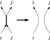
If the singular edge $E$ has degree $=0$, take two colored paths outgoing from $E$ and incoming to the same singular edge ( or incoming to $E$ and outgoing from the same singular edge). If the degrees of the singular edges on the colored paths except the source and target vertices are not changed by exchanging the colorings of these colored paths, exchange the colorings of the colored paths. These conditions implies that the source or the target singular edge which is not $E$ must not be positive type and the degree of its singular edge must be shifted $+1$, and the degree of the singular edge $E$ is changed to $-1$. So we can replace the singular edge $E$ to the parallel normal edges and consider it as an element of $C(\Gamma^{0})$. We denote it as $\sigma^{\prime}\in C(\Gamma^{0})$. We only permit color exchanging which satisfies $\mathrm{gr}(\sigma)=\mathrm{gr}(\sigma^{\prime})$. If there are some possibilities of exchanging the colorings, sum up all of them. If there are no possibilities of changing which satisfy the conditions, we consider the value as $0$.

In the $\chi_{0}$ case, we would like to construct a morphism $C(\Gamma^{0})\longrightarrow C(\Gamma^{1})$ which is similar to $\chi_{1}$. Fix an element $\sigma\in C(\Gamma^{0})$ and consider $\sigma$ as colored oriented trivalent planar graph.

Assume that the parallel normal edges of $\sigma$ have colorings $i\geq j$ depicted as in the Fig. 15 and put a dotted circle around the parallel normal edges. This putted circle can be seen as a dotted line as in the left-hand side of the figure {fig. We may treat a dotted circle like a singular edge. Take two colored paths which start from same singular edge (or the dotted circle around the parallel edges) and end at same singular edge (or the dotted circle around the parallel normal edges). We assume that one of the colored paths contains the normal edge of parallel edges colored $i,\ or\ j$. These two path can be seen as a colored subgraph of $\sigma$ and we impose them not to have self-intersections and not to have a path which crosses this subgraph whose intersection points with this subgraph are positive singular edges or negative singular edges. So paths which traverse the subgraph are allowed to have only degree zero intersection points. We also call them as distinguished subgraph. (By considering the dotted circle as singular edge, a distinguished subgraph can be seen as a distinguished circle which is used in the $\chi_{1}$ case.) Exchanging colorings of colored paths of a distinguished subgraph will introduce a new distinguished subgraph and a new colored oriented graph.

Take a distinguished circle of $\sigma$ whose source and terminal singular edges are not positive. If exchanging colorings of the distinguished subgraph does not change the degrees of the singular edges on the distinguished subgraph except the source and target singular edges (or the dotted circle as source or target singular edge of distinguished subgraph), we will exchange the colorings of colored paths of the distinguished subgraph and replace the parallel normal edges to the singular normal edge $E$ by the natural way as in the Fig. 11. We can consider it as an element of $C(\Gamma^{1})$. We will modify and add other term as the special case. We must add and consider exceptional terms to $\chi_{0}$ which is related to the Reidemeister 1-move. If the normal edges of parallel edges colored $i$ or $j$ consist a simple loop, replace the parallel normal edges to singular edges and change the coloring of simple closed curve as to preserve the grade as in the $\chi_{1}$ case.

If the subgraph does not permit these procedure (or there are no such subgraph satisfying the conditions), we send them to $0$. If there are some possibilities of taking distinguished subgraphs and exchanging the colorings, sum up all of them.

Suppose the parallel edges of $\sigma$ colored $i,\ j$ depicted in the Fig. 15 has a relation $i<j$, replace the parallel normal edges to a singular edge $E$ and naturally extend its colorings. This singular edge $E$ has the degree $1$ and we will consider them as an element of $C(\Gamma^{1})$.

So, $\chi_{0}$ and $\chi_{1}$ change some gradings of singular edges and colorings of normal edges. They are degree$=0$ morphisms by definitions.

Let $k$ be an integer. We denote by $\{k\}$ the grading shift up by $k$. (i,e. Let $\sigma\in C(G)$ be a colored graph and $\mathrm{gr}(\sigma)=n$, then $\sigma\{k\}\in C(G)\{k\}$ has the grading $\mathrm{gr}(\sigma)=n+k$.) We denote the some propositions which are called MOY relations developed by Murakami, Ohtsuki and Yamada [5].

These propositions are the consequence of [5], derived from the representation of quantum group and its $R$-matrix , also have close connection to the theory of Kazhdan-Lusztig basis of Hecke algebras but we shall not pursue this line of thought. We omit the proofs.

For a link diagram $D$ and $Cr\supset cr$ be a crossing set, we have constructed a complex associated with $C(D(cr)),\ \chi_{0},\ \chi_{1}$. We assume to locate $C(D(cr))$ at the cohomological degree$=N_{1}^{+}-N_{0}^{-}$, and we will denote by $C^{*}(D)$ the complex associated with the diagram constructed by the shifted cube structure. We state the main theorem whose proof is stated in the next section.

Consider the type-I Reidemeister move.

Consider diagrams $D$ and $D^{\prime}$ depicted in the figure21.

Consider diagrams $D,\ D^{\prime}$ which is almost same but different only in the small area depicted in the Fig. 23.

We will prove the following proposition.

References

- [1] M. Khovanov, Categorification of the Jones polynomial, Duke J. of Math. (2000), 359–426.
- [2] M. Khovanov, L. Rosansky, Matrix factorizations and link homology, Fundamenta Mathematicae. vol.199 (2008), 1-91.
- [3] M. Khovanov, L. Rozansky, Matrix factorizations and link homology 2, Geometry and Topology. vol.12 (2008), 1387-1425.
- [4] M. Khovanov, L. Rozansky, Triply-graded link homology and Hochschild homology of Soergel bimodules, International Journal of Math. vol.18, no.8 (2007), 869-885.
- [5] C. Manolescu, Link homology theories from symplectic geometry, Advances in Mathematics, Vol. 211 (2007), 363-416
- [6] H. Murakami, T. Ohtsuki, S. Yamada, Homfly polynomial via an invariant of colored plane graphs, Enseign.Math. (2) 44 (1998), 325–360.
- [7] V.G. Turaev, The Yang-Baxter equation and invariants of links, Invent. Math. 92 (1988), 527–553.
- [8] H. Wu, Generic deformations of the colored -homology for links. preprint.
Osaka City University
E-mail address: d07sag0702@ex.media.osaka-cu.ac.jp