Thermal leptogenesis and the gravitino problem in the
Asaka-Yanagida axion/axino dark matter scenario

The only relevant MSSM parameters for our analysis are the $\widetilde{Z}_{1}$ and $\widetilde{G}$ masses $m_{\widetilde{Z}_{1}}$ and $m_{\widetilde{G}}$, the $\widetilde{Z}_{1}$ bino component $v_{4}^{(1)}$ in the notation of [6], and the $\widetilde{Z}_{1}$ abundance after freeze-out $\Omega_{\widetilde{Z}_{1}}$. The remaining of the MSSM parameters only impact the running of the gauge couplings and the value of $\Omega_{\widetilde{G}}$, which depend on all the gaugino masses (see Eq. (6) below). However, as shown below, in the AY scenario with $T_{R}\gtrsim 10^{9}$ GeV, the contribution from $\widetilde{G}\rightarrow a\tilde{a}$ decay to the dark matter relic density is negligible. Thus the dependence on the entire SUSY spectrum is very mild.

For illustration we will use a generic mSUGRA scenario with $m_{0}=1000$ GeV, $m_{1/2}=1000$ GeV, $A_{0}=0$, $\tan\beta=55$ and $\mu>0$, which gives $m_{\widetilde{Z}_{1}}=430$ GeV and $\Omega_{\widetilde{Z}_{1}}=0.04$, but treat $m_{\widetilde{Z}_{1}}$ and $\Omega_{\widetilde{Z}_{1}}$ as free parameters throughout most of the numerical analysis. The bino component of the $\widetilde{Z}_{1}$ wavefunction is important, since it determines the $\widetilde{Z}_{1}-\tilde{a}$ coupling. For simplicity we will assume a purely bino neutralino, which is valid for a large portion of the mSUGRA parameter space. We also take $m_{\widetilde{G}}=m_{\widetilde{Z}_{1}}/2$ and $m_{\tilde{a}}<m_{\widetilde{G}}$ in order to have an axino LSP with a gravitino NLSP.

Here, we consider four mechanisms for dark matter production in the AY scenario.

• •

  If the reheat temperature $T_{R}$ exceeds the axino decoupling temperature

  $$T_{dcp}=10^{11}\ {\rm GeV}\left(\frac{f_{a}/N}{10^{12}\ {\rm GeV}}\right)^{2}\left(\frac{0.1}{\alpha_{s}}\right)^{3},$$

  (2)

  axinos will be in thermal equilibrium, with an abundance given by

  $$\Omega_{\tilde{a}}^{TE}h^{2}\simeq 0.38\left(\frac{m_{\tilde{a}}}{1\ {\rm keV}}\right).$$

  (3)

  To avoid overproducing axino dark matter, the RTW bound [25] then implies that $m_{\tilde{a}}<0.3$ keV.

  In the case where $T_{R}<T_{dcp}$, the axinos are never in thermal equilibrium in the early universe. However, they can still be produced thermally via radiation off of particles that are in thermal equilibrium [27, 28]. Here, we adopt a recent calculation of the thermally produced (TP) axino abundance from Strumia [29]:

  $$\Omega_{\tilde{a}}^{\rm TP}h^{2}=1.24g_{3}^{4}F(g_{3})\frac{m_{\tilde{a}}}{{\rm GeV}}\frac{T_{R}}{10^{4}\ {\rm GeV}}\left(\frac{10^{11}}{f_{a}/N}\right)^{2},$$

  (4)

  with $F(g_{3})\sim 20g_{3}^{2}\ln\frac{3}{g_{3}}$, and $g_{3}$ is the strong coupling constant evaluated at $Q=T_{R}$.

• •

  In supersymmetric scenarios with a quasi-stable neutralino, the $\widetilde{Z}_{1}$s will be present in thermal equilibrium in the early universe, and will freeze out when the expansion rate exceeds their interaction rate, at a temperature roughly $T_{fo}\sim m_{\widetilde{Z}_{1}}/20$. The present day abundance can be evaluated by integrating the Boltzmann equation. Several computer codes are available for this computation. Here we use the code IsaReD [30], a part of the Isajet/Isatools package [31, 32].

  In our case, each neutralino will undergo decay to the stable axino LSP, via decays such as $\widetilde{Z}_{1}\rightarrow\tilde{a}\gamma$. Neutralinos may also decay via e.g. $\widetilde{Z}_{1}\rightarrow\widetilde{G}\gamma$, but these modes are suppressed by $1/m_{Pl}^{2}$ rather than $1/(f_{a}/N)^{2}$, and so the decay to gravitinos is suppressed (one of the hallmarks of the AY scenario). Thus, the non-thermally produced (NTP) axinos will inherit the thermally produced neutralino number density, and we will simply have [27]

  $$\Omega_{\tilde{a}}^{\widetilde{Z}}h^{2}=\frac{m_{\tilde{a}}}{m_{\widetilde{Z}_{1}}}\Omega_{\widetilde{Z}_{1}}^{TP}h^{2}.$$

  (5)

• •

  Since here we are attempting to generate reheat temperatures $T_{R}\gtrsim 10^{9}$ GeV, we must also include in our calculations the thermal production of gravitinos in the early universe. We adopt the calculation of Pradler and Steffen in Ref. [33], who have estimated the thermal gravitino production abundance as

  $$\Omega_{\widetilde{G}}^{\rm TP}h^{2}=\sum_{i=1}^{3}\omega_{i}g_{i}^{2}(T_{R})\left(1+\frac{M_{i}^{2}(T_{R})}{3m_{\widetilde{G}}^{2}}\right)\ln\left(\frac{k_{i}}{g_{i}(T_{R})}\right)\left(\frac{m_{\widetilde{G}}}{100\ {\rm GeV}}\right)\left(\frac{T_{R}}{10^{10}\ {\rm GeV}}\right),$$

  (6)

  where $\omega_{i}=(0.018,0.044,0.117)$, $k_{i}=(1.266,1.312,1.271)$, $g_{i}$ are the gauge couplings evaluated at $Q=T_{R}$ and $M_{i}$ are the gaugino masses also evaluated at $Q=T_{R}$. For the temperatures we are interested in, this agrees within a factor of about 2 with the more recent calculation by Rychkov and Strumia [33], which is sufficient for our purposes.

  Since the only kinematically allowed gravitino decay mode is to an axion plus an axino LSP, the abundance of axinos from gravitino production is given by

  $$\Omega_{\tilde{a}}^{\widetilde{G}}h^{2}=\frac{m_{\tilde{a}}}{m_{\widetilde{G}}}\Omega_{\widetilde{G}}^{TP}h^{2},$$

  (7)

  while the abundance of axions from gravitino production is given by

  $$\Omega_{a}^{\widetilde{G}}h^{2}=\frac{m_{a}}{m_{\widetilde{G}}}\Omega_{\widetilde{G}}^{TP}h^{2}.$$

  (8)

  For axino masses in the MeV range and gravitino masses in the TeV range, the prefactor above is extremely small, making the contribution from gravitino decays to the axino relic abundance negligible, what allows us to evade overproduction of dark matter via thermal gravitino production.

• •

  Here, we consider the scenario where the PQ symmetry breaks before the end of inflation, so that a nearly uniform value of the axion field $\theta_{i}\equiv a(x)/(f_{a}/N)$ is expected throughout the universe. The axion field equation of motion implies that the axion field stays relatively constant until temperatures approach the QCD scale $T_{QCD}\sim 1$ GeV. At this point, the temperature-dependent axion mass term turns on, and a potential is induced for the axion field. The axion field rolls towards its minimum and oscillates, filling the universe with low energy (cold) axions. The expected axion relic density via this vacuum mis-alignment mechanism is given by [34]

  $$\Omega_{a}h^{2}\simeq 0.23f(\theta_{i})\theta_{i}^{2}\left(\frac{f_{a}/N}{10^{12}\ {\rm GeV}}\right)^{7/6}$$

  (9)

  where $0<\theta_{i}<\pi$ and $f(\theta_{i})$ is the so-called anharmonicity factor. Visinelli and Gondolo [34] parametrize the latter as $f(\theta_{i})=\left[\ln\left(\frac{e}{1-\theta_{i}^{2}/\pi^{2}}\right)\right]^{7/6}$. The uncertainty in $\Omega_{a}h^{2}$ from vacuum mis-alignment is estimated as plus-or-minus a factor of three.

In this paper, we will evaluate the mixed axion/axino relic density from the above four sources:

Over much of parameter space, if $m_{\tilde{a}}$ is taken to be of order the MeV scale or below, then the contributions $\Omega_{\tilde{a}}^{\widetilde{G}}$, $\Omega_{\tilde{a}}^{\widetilde{Z}_{1}}$ and $\Omega_{a}^{\widetilde{G}}$ are subdominant.

In Fig. 1, we illustrate in frame a) the relative importance of the four individual contributions as a function of $f_{a}/N$, for $\Omega_{\widetilde{Z}_{1}}h^{2}=10$, $m_{\widetilde{Z}_{1}}=430$ GeV and $m_{\widetilde{G}}=0.5m_{\widetilde{Z}_{1}}$. For the axion/axino sector we take $\theta_{i}=0.05$ and $m_{\tilde{a}}=100$ keV. The value of $T_{R}$ is adjusted such that $\Omega_{a\tilde{a}}h^{2}=0.1123$. Low values of $\theta_{i}$ suppress axion production and allow higher values of $f_{a}/N$ to be probed; the higher values of $f_{a}/N$ suppress thermal axino production, thus allowing for higher $T_{R}$ values to compensate.

For low $f_{a}/N$ values, the TP axino contribution is dominant. But as $f_{a}/N$ increases, the axion component grows. For higher values of $f_{a}/N$, the vacuum-misalignment produced axion component dominates, and the dark matter is predominantly composed of cold axions. The contribution of axino dark matter from $\widetilde{Z}_{1}$ and $\widetilde{G}$ decays are always negligible in this case.

In frame b) of Fig. 1, we show the value of $T_{R}$ which is needed to enforce the total abundance of mixed axion/axino dark matter to be $\Omega_{a\tilde{a}}h^{2}=0.1123$. We show cases for $m_{\tilde{a}}=0.1$ and 1 MeV. As $f_{a}/N$ increases, the axino-matter coupling decreases, and one would expect the thermal production of axinos to decrease. Since we enforce $\Omega_{a\tilde{a}}h^{2}=0.1123$, then higher values of $T_{R}$ are needed to compensate and enhance the thermal production of axinos[35] (and gravitinos). We see that the value of $T_{R}$ can be pushed to over $10^{9}$ GeV for $m_{\tilde{a}}=1$ MeV, and to over $10^{10}$ GeV for $m_{\tilde{a}}=0.1$ MeV, thus allowing high enough $T_{R}$ for thermal leptogenesis.

Depending on its mass, the axino might constitute warm (WDM) or hot (HDM) dark matter; the latter possibilities are severely constrained by the matter power spectrum and reionization [27, 36] (see also [37, 38]). We consider axinos with mass $1-100$ keV as mostly WDM, and axinos with mass $<1$ keV as mostly HDM. Since these bounds on the amount of WDM/HDM are model dependent [36], we do not impose strict WDM/HDM constraints on our results. However, for guidance, we will keep track of PQMSSM parameter points with potentially too large WDM and/or HDM components¹¹ 1 Axions produced from gravitino decay will also constitute HDM. However, since this contribution to the total DM density is suppressed by $m_{a}/m_{\widetilde{G}}$, it can be safely neglected.: As in [12], we disfavour points with

where $\Omega_{\tilde{a}}=\Omega_{\tilde{a}}^{TP}+\Omega_{\tilde{a}}^{\widetilde{G}}+\Omega_{\tilde{a}}^{\widetilde{Z}}$. This is rather conservative. A rough estimate based on the neutrino mass limit [38] from cosmological data, $\sum m_{\nu}<0.41$ to $0.44$ eV, gives that up to 4–5% HDM contribution could be acceptable. Moreover, Boyarsky et al. in [37] found that in case of a thermal relic (TR), 100% WDM is allowed for $m_{\rm TR}\geq 1.7$ keV, while for $m_{\rm TR}=1.1$ keV as much as 40% WDM is allowed at 95% CL. We will also indicate these bounds, which are considerably weaker than Eq. (11).

The AY scenario naturally avoids BBN constraints on late decaying gravitinos by assuming the mass relation $m({\rm sparticle})>m_{\widetilde{G}}>m_{\tilde{a}}$, so that the $\widetilde{G}$ decays inertly 100% of the time into $a\tilde{a}$. However, by searching for PQMSSM parameters which allow $T_{R}\gtrsim 2\times 10^{9}$ GeV while avoiding overproduction of mixed axino/axion dark matter (the latter requires large $f_{a}/N\sim 10^{12}$ GeV and small $\theta_{i}$), we have pushed the $\widetilde{Z}_{1}$ lifetime uncomfortably high, so that its hadronic decays in the early universe now have the potential to disrupt BBN. The $\widetilde{Z}_{1}$ lifetime and hadronic branching fraction is calculated in Ref. [27, 12].

Constraints from BBN on hadronic decays of long-lived neutral particles in the early universe have been calculated in Ref’s [39, 40, 41]. Here, we adopt the results from Jedamzik [41]. The BBN constraints arise due to injection of high energy hadronic particles into the thermal plasma during or after BBN. The constraints depend on three main factors:

• •

  The abundance of the long-lived neutral particles. In Ref. [41], this is given by $\Omega_{X}h^{2}$ where $X$ is the long-lived neutral particle which undergoes hadronic decays. In our case, where the long-lived particle is the lightest neutralino which decays to an axino LSP, this is just given by the usual thermal neutralino abundance $\Omega_{\widetilde{Z}_{1}}h^{2}$, as calculated by IsaReD [30].

• •

  The lifetime $\tau_{X}$ of the long-lived neutral particle. The longer-lived $X$ is, the greater its potential to disrupt the successful BBN calculations. In our case $\tau_{X}=\tau_{\widetilde{Z}_{1}}\propto(f_{a}/N)^{2}/m_{\widetilde{Z}_{1}}^{3}$.

• •

  The hadronic branching fraction $B_{h}$ of the long-lived neutral particle. If this is very small, then very little hadronic energy will be injected, and hence the constraints should be more mild.

From the above list, we see that BBN directly constrains the MSSM parameters ($\Omega_{\widetilde{Z}_{1}}h^{2}$ and $m_{\widetilde{Z}_{1}}$) of the PQMSSM model. The constraints also depend on $f_{a}$, since its value directly affects $\tau_{\widetilde{Z}_{1}}$. The BBN constraints are shown in Fig. 9 (for $m_{X}=1$ TeV) and Fig. 10 (for $m_{X}=100$ GeV) of Ref. [41], as contours in the $\tau_{X}\ vs.\ \Omega_{X}h^{2}$ plane, with numerous contours for differing $B_{h}$ values ranging from $10^{-5}$ to 1. For $B_{h}\sim 0.1$, for instance, and very large values of $\Omega_{X}h^{2}\sim 10-10^{3}$, the lifetime $\tau_{X}$ must be $\lesssim 0.1$ sec, or else the primordial abundance of ${}^{4}\rm He$ is disrupted. If $\Omega_{X}h^{2}$ drops below $\sim 1$, then much larger values of $\tau_{X}$ up to $\sim 100$ sec are allowed. If one desires a long-lived hadronically decaying particle in the early universe with $\tau_{X}\gtrsim 100$ sec, then typically much lower values of $\Omega_{X}h^{2}\sim 10^{-6}-10^{-4}$ are required.

We have digitized the constraints of Ref. [41], implementing extrapolations for cases intermediate between values of parameters shown, so as to approximately apply the BBN constraints to the AY scenario with a long-lived neutralino decaying during BBN. The results are shown in Fig. 2, as a function of $m_{\widetilde{Z}_{1}}$. From Fig. 1b), we have $T_{R}>10^{9}$ GeV for $f_{a}/N\sim 10^{13}$ GeV. From Fig. 2, we see that, for $m_{\widetilde{Z}_{1}}\sim 400$ GeV and $f_{a}/N=10^{13}$ GeV, we need $\Omega_{\widetilde{Z}_{1}}h^{2}<0.4$ in order to satisfy the BBN bounds. In particular, the assumed value for $\Omega_{\widetilde{Z}_{1}}h^{2}$ (=10) in Fig. 1 only satisfies the BBN constraints for $f_{a}/N\lesssim 2\times 10^{12}$ GeV or $T_{R}\lesssim 3\times 10^{8}$ GeV. Therefore we see that the AY scenario with $T_{R}\gtrsim 10^{9}$ GeV requires quite low values of $\Omega_{\widetilde{Z}_{1}}h^{2}$ and/or a heavy $\widetilde{Z}_{1}$.

The results of the last section were for a specific choice of the axino mass and $\theta_{i}$ values. Next, we examine which values of $T_{R}$ are possible for arbitrary values of $f_{a}$, $m_{\tilde{a}}$ and $\theta_{i}$. For now we keep the MSSM parameters ($\Omega_{\widetilde{Z}_{1}}h^{2}$ and $m_{\widetilde{Z}_{1}}$) fixed. As discussed in the previous section, the BBN constraints in general require low $\Omega_{\widetilde{Z}_{1}}h^{2}$ and high $m_{\widetilde{Z}_{1}}$. We therefore assume $\Omega_{\widetilde{Z}_{1}}h^{2}=0.04$ and $m_{\widetilde{Z}_{1}}=430$ GeV, which are values consistent with, e.g., an mSUGRA point near the apex of the Higgs funnel region. To probe the full PQ parameter space we perform a random scan over the PQ parameters in the range

and calculate the value of $T_{R}$ which is needed to enforce $\Omega_{a\tilde{a}}h^{2}=0.1123$. The results of our scan are shown in Fig. 3, where we plot the derived value of $T_{R}$ versus PQ breaking scale $f_{a}/N$. In the plot, dark blue and dark red points have mainly CDM with at most 20% WDM and at most 1% HDM admixture, c.f. Section 2.3. The light blue and light red points have higher values of WDM or HDM. The red points are excluded by bounds derived from Ref. [41] on late decaying neutralinos which could destroy the succesful predictions of BBN. Blue points are allowed by BBN constraints. Applying the WDM bounds of Boyarsky et al.[37] for a thermal relic and allowing up to 5% HDM, the boundary between dark and light blue points moves left to the dashed blue line.

We do see that a number of dark blue points with mainly CDM, and which also respect BBN bounds, can be generated with $T_{R}>2\times 10^{9}$ GeV. These thermal leptogenesis-consistent points all require $f_{a}/N\gtrsim 10^{12}$ GeV (or $f_{a}/N\gtrsim 6\times 10^{11}$ GeV with weaker WDM/HDM requirements).

In Fig. 4, we show the same scan in the $\theta_{i}\ vs.\ T_{R}$ plane. Here, we see that the CDM/BBN consistent points with high $T_{R}$ all need rather small values of axion mis-alignment angle $\theta_{i}\lesssim 0.5$. This is needed since, at large $T_{R}$, large $f_{a}/N$ is necessary to suppress overproduction of axinos, while small $\theta_{i}$ is needed to suppress over-production of axions.

In Fig. 5, we show the same PQMSSM parameter scan for $m_{\widetilde{Z}_{1}}=430$ GeV and $\Omega_{\widetilde{Z}_{1}}h^{2}=0.04$, but in the $\Omega_{a}h^{2}\ vs.\ T_{R}$ plane. Here, we see that the CDM/BBN consistent points with high $T_{R}$ can have both large and small values of $\Omega_{a}h^{2}$. Solutions with $\Omega_{a}h^{2}\sim 0.1$ usually have very light axinos (to suppress $\Omega_{\tilde{a}}h^{2}$) and moderate $\theta_{i}$ values. Solutions with $\Omega_{a}h^{2}\lesssim 0.1$ usually have heavier axinos and small $\theta_{i}$.

While the results of the previous figures are restricted to specific values of $m_{\widetilde{Z}_{1}}$ and $\Omega_{\widetilde{Z}_{1}}h^{2}$, the overall scheme is much more general. The lesson here is that the AY scenario for reconciling thermal leptogenesis with the gravitino problem can work provided certain conditions on SUSY models are met. These conditions are rather similar to those needed by the large $m_{3/2}$ scenario put forth in Ref. [12]. After adopting a model with a sparticle mass hierarchy of $m({\rm sparticles})>m_{\widetilde{G}}>m_{\tilde{a}}$, with $m_{\tilde{a}}\sim$MeV scale and $m_{\widetilde{G}}\sim M_{{\rm weak}}$, one needs the following features:

• •

  To allow for $T_{R}>2\times 10^{9}$ GeV, one must suppress thermal production of axinos via a large value of $f_{a}/N\gtrsim 10^{12}$ GeV.

• •

  To suppress overproduction of axions one must adopt a lower range of mis-alignment angle $\theta_{i}\lesssim 0.5$ (or $\theta_{i}\lesssim 0.8$ taking into account the factor 3 uncertainty in Eq. (9)) .

• •

  The large value of $f_{a}/N$ increases the $\widetilde{Z}_{1}$ lifetime, which brings in BBN constraints on late-decaying neutral particles. To avoid BBN bounds, it helps to invoke 1. a bino-like $\widetilde{Z}_{1}$ so that $v_{4}^{(1)}\sim 1$, 2. a low apparent neutralino relic abundance $\Omega_{\widetilde{Z}_{1}}^{app}h^{2}\lesssim 1$ and 3. a large value of $m_{\widetilde{Z}_{1}}$ to help suppress the $\widetilde{Z}_{1}$ lifetime.

As mentioned above, if $T_{R}$ exceeds $T_{dcp}$ in the early universe, saxions are produced in thermal equilibrium such that

where $s=2\pi^{2}g_{*}T^{3}/45$ is the plasma entropy density and $Y_{s}$ is the saxion yield. For $T_{R}<T_{dcp}$, saxions can still be produced thermally, although to our knowledge a full calculation is not yet available. In Ref’s [22] and [45], thermal saxion production is estimated to be

which we will adopt for our calculations.

In addition, saxions can be produced via coherent oscillations of the saxion field in the early universe. Although the exact mechanism depends on the saxion potential near the SUSY breaking scale, the energy density associated with the coherent oscillations can be parametrized by the initial saxion field strength, $s_{i}$. Natural values for $s_{i}$ are $s_{i}\sim f_{a}$ or $s_{i}\sim M_{Pl}$. Unless stated otherwise, we will assume $s_{i}=f_{a}/N$. The saxion energy density is estimated for the case of very high values of $T_{R}$ with $\Gamma_{I}>m_{s}$ (here, $T_{R}$ is related to the inflaton decay width $\Gamma_{I}$ as $T_{R}=(3/g_{*}\pi^{3})^{1/4}(M_{Pl}\Gamma_{I})^{1/2}$) as [45]

while for $\Gamma_{I}<m_{s}$,

The summed saxion abundance is then given by the thermal production if $T_{R}>T_{dcp}$ or by the sum of thermal production plus the abundance from coherent oscillations, if $T_{R}<T_{dcp}$.

As an example, we show in Fig. 7 the saxion yield $Y_{s}$ versus $f_{a}/N$ for $m_{s}=0.1$ and 1 TeV and for $T_{R}=10^{9}$ GeV. At low $f_{a}/N$, $T_{R}>T_{dcp}$, and saxions are produced in thermal equilibrium. Once $T_{dcp}$ rises above $T_{R}$, thermal saxion production dominates, but decreases with increasing $f_{a}/N$ until the point where saxion production from coherent oscilations dominates.

The saxion is an $R$-parity even state which is expected to dominantly decay into two gluons: $s\rightarrow gg$. The saxion decay width differs by factors of two in Ref’s [46], [22] and [45]. By an independent calculation, we find

in agreement with [22]. The saxion may also decay (or not, model dependently) via $s\rightarrow aa$, and in the DFSZ[16] model, into $q\bar{q}$ or $\ell\bar{\ell}$. These latter decays are suppressed in the KSVZ model[15]. Saxion may also decay to $\widetilde{Z}_{i}\widetilde{Z}_{j}$, $\gamma\gamma$ and $\tilde{g}\tilde{g}$. For saxion decay to gluino pairs, we calculate the interaction as²² 2 Our saxion-gluino-gluino interaction differs by a factor of 2 from Ref. [29].

and then find

The two widths are compared in Fig. 8, where the $s\rightarrow gg$ decay is found to always dominate.

The temperature associated with saxion decay and entropy injection is given by [47]

All the saxion decays essentially finish entropy injection by the time the universe cools to this value[47]. For simplicity, here we will assume the $\Gamma_{s}=\Gamma(s\rightarrow gg)$ so that our results are independent of $m_{\tilde{g}}$. Folding in the additional strong decay $s\rightarrow\tilde{g}\tilde{g}$ will result typically in a small increase in $T_{s}$. In Fig. 9, we plot the value $T_{s}$ as a function of $f_{a}/N$ for three different values of the saxion mass.

Armed with expressions for the saxion production rate in the early universe, we next calculate the temperature $T_{e}$ at which the saxion energy density in the universe equals the plasma energy density:

Using $\rho_{s}=m_{s}Y_{s}s$ and $s=\frac{2\pi^{2}}{45}g_{*}T^{3}$, we find

If $T_{e}$ exceeds $T_{s}$ (i.e. if saxion domination occurs before saxion decay), then saxions dominate the energy density of the universe for $T_{s}\lesssim T\lesssim T_{e}$. In this case, saxion decays may inject significant entropy and dilute whatever abundances are present at temperature $T_{s}$. The situation is shown in Fig. 10, where we show the value of $T_{s}$ (blue horizontal lines) and the value of $T_{e}$ (red lines) for $f_{a}/N=10^{12}$ and $10^{14}$ GeV. For $T_{R}$ greater than the $r=1$ intersection points, significant entropy injection can occur.

If $r>1$, $T_{s}$ must satisfy $T_{s}\gtrsim 10$ MeV, so the universe becomes radiation dominated before BBN starts. On the other hand, if $r<1$, the early universe is always radiation dominated and the usual BBN constraints on late decaying particles can be applied[41], as in the case of neutralino decays. If the conditions $10\ {\rm MeV}<T_{s}$ and $T_{e}>T_{s}$ hold, then saxion decay can inject substantial entropy and dilute whatever relics are present and decoupled from the thermal plasma at the time of saxion decay ($T=T_{s}$). The ratio of entropy injection before and after a quasi-stable particle decay, for a matter dominated universe ($T_{e}>T_{s}$), has been calculated in Scherrer and Turner[47], and is given by

where $\bar{g}_{*}$ is the number of relativistic degrees of freedom averaged over the saxion decay period, which we approximate by $g_{*}(T_{s})$. The above expression for $r$ is only valid for $T_{e}>T_{s}$ (saxion dominated universe) or $r>1$. However, if the saxion energy density never dominates the universe, the entropy injection is negligible[47]. Therefore we assume $r=1$ (no entropy injection), if $T_{e}<T_{s}$.

Assuming $\Gamma_{s}$ is dominated by the $s\rightarrow gg$ decay, we plot in Fig. 11a) the value of $r$ in the $(f_{a}/N)\ vs.\ T_{R}$ plane for $m_{s}=0.1,\ 1\ {\rm and}\ 10$ TeV, assuming $s_{i}/(f_{a}/N)=1$ (for production from coherent oscillations). The solid lines all maintain $T_{s}>10$ MeV, while dashed lines violate this constraint. We see first that for $m_{s}=100$ GeV, significant entropy production only occurs for $f_{a}/N\lesssim 4\times 10^{11}$ GeV; for larger $f_{a}/N$, $\Gamma_{s}$ is suppressed and the saxion lives long enough to decay during or after BBN. For $m_{s}=1$ TeV, entropy injection can occur for $f_{a}/N\lesssim 10^{13}$ GeV.

If $T_{R}$ lies below the $r=1$ contours, then not much entropy is injected, but for high $T_{R}$, large entropy injection is possible and must be accounted for. The various contours of constant $r$ initially increase with $T_{R}$. In this case, the saxion production is dominantly thermal. When the curves turn over, saxion production is dominated by coherent oscillations. In this case, as $f_{a}/N$ increases, the saxion field strength also increases (since $s_{i}/(f_{a}/N)$ is fixed to 1), and much lower $T_{R}$ values are allowed for substantial entropy production. Another noteworthy feature is that the contours of entropy production increase with $T_{R}$ as $m_{s}$ increases. Thus, the dilution of DM from saxion decay can be reduced by requiring rather heavy saxions. Finally, when we compare Fig. 3 to Fig. 11, we see that the range of $T_{R}\sim 10^{9}-10^{11}$ GeV for $f_{a}/N\sim 10^{12}-10^{14}$ implies that entropy dilution from saxion decay needs to be accounted for in our calculations for the case where $s_{i}/(f_{a}/N)\sim 1$ and $m_{s}=m_{0}=1$ TeV.

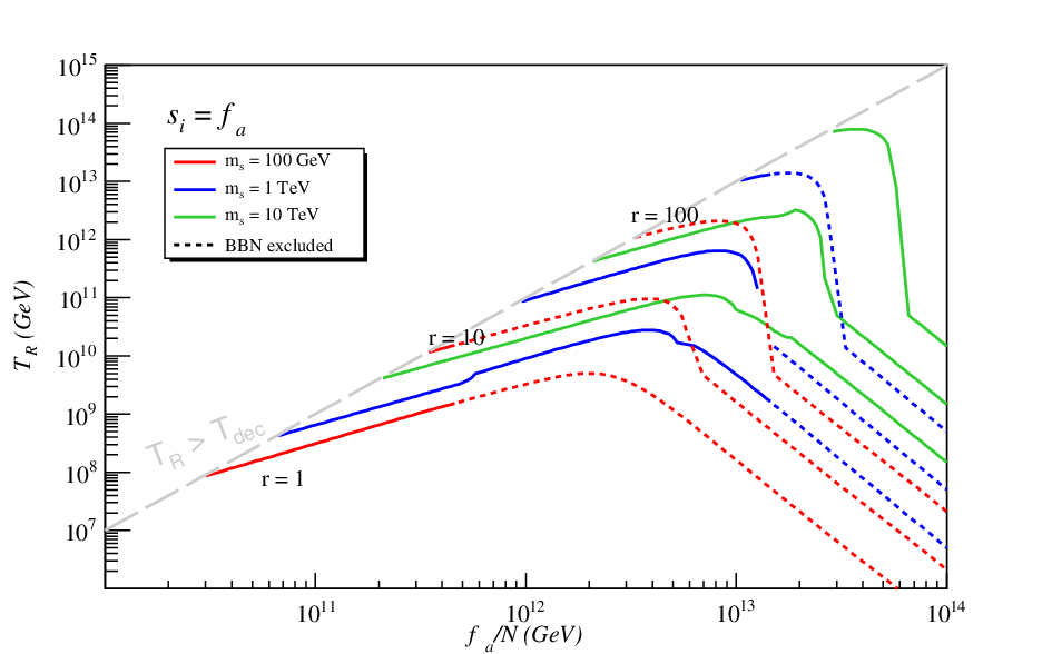
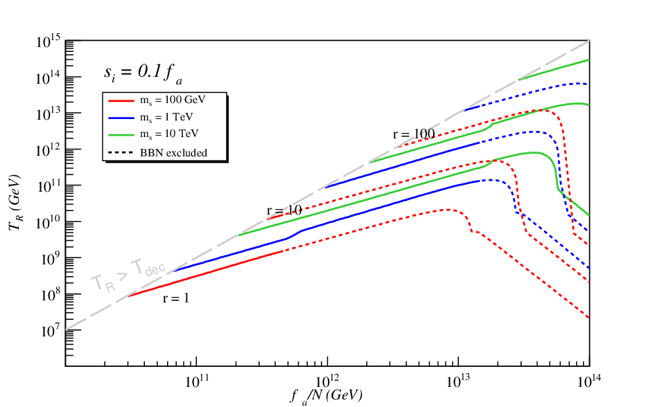
In Fig. 11b), we plot again the entropy ratio contours, but this time taking $s_{i}/(f_{a}/N)=0.1$. In this case, saxion production from coherent oscillations is suppressed by the smaller initial saxion field strength value. This expands the range of large $T_{R}$ at high $f_{a}/N$ where entropy injection is negligible. In cases such as these, the results of the previous section (and also Ref. [12]) remain viable, and entropy injection from saxion decay would be a negligible effect. From here on, we will assume $s_{i}/(f_{a}/N)=1$.

As mentioned before, the entropy injection from late decaying saxions will dilute the number density of any particle decoupled from the thermal plasma at $T=T_{s}$. Therefore, depending on $T_{s}$, the saxion production and decay may dilute thermally produced axinos, gravitinos, the quasi-stable $\widetilde{Z}_{1}$s, sometimes the axions and of course the matter-antimatter asymmetry itself. In this latter case, the baryon-to-photon ratio $\eta_{B}\equiv n_{B}/n_{\gamma}$ is diluted to a value $\eta_{B}/r$.

To accommodate the latter possibility, we note that the lepton asymmetry and consequently the baryon assymetry is proportional to the mass of the lightest right-handed neutrino, $M_{1}$ (assuming $M_{1}\ll M_{2,3}$)[48]. Therefore, to compensate the saxion dilution, heavier neutrinos are necessary. Since thermal leptogenesis requires $T_{R}>M_{1}$, in the case of saxion entropy injection, we need $T_{R}>r\times(2\times 10^{9})$ GeV.

To include the above effects into our new analysis, we adopt the following procedure:

• •

  Calculate the thermal plus coherent oscillation yield of saxions $Y_{s}$ in the early universe.

• •

  Calculate the saxion decay temperature $T_{s}$.

• •

  Calculate $T_{e}$ and determine if saxions can dominate the universe ($T_{e}>T_{s}$).

• •

  Calculate the final/initial entropy ratio $r$.

• •

  If $r<1$, then the entropy injection is negligible and we require the saxion lifetime and relic density to satisfy the BBN bounds for late decaying particles in a radiation dominated universe,

• •

  If $T_{s}<10$ MeV and $r>1$, then the point is excluded due to entropy injection during or after BBN.

• •

  If $T_{s}>10$ MeV and $r>1$,

  • –

    dilute thermally produced axinos by factor $r$.

  • –

    dilute thermally produced gravitinos by $r$.

  • –

    If $T_{s}<T_{QCD}=1$ GeV, dilute mis-alignment produced axions by $r$.

  • –

    If $T_{s}<T_{fo}=m_{\widetilde{Z}_{1}}/25$, dilute quasi-stable neutralinos by $r$. This condition can dilute axinos produced by neutralino decay, but also impacts the quasi-stable neutralino BBN bounds from Fig. 2.

Our first results are shown in Fig. 12 for the same PQMSSM parameters used in Fig. 1, but including saxion entropy injection with $m_{s}=1$ TeV. In frame a), we plot the relic abundance of thermally produced axinos (red), axions (blue), gravitino produced axinos (lavender) and neutralino produced axinos (magenta). The value of $T_{R}$ is always adjusted to maintain $\Omega_{a\tilde{a}}=0.1123$, and so $T_{R}/r$ is shown in frame b) for $m_{\tilde{a}}=0.1$ and 1 MeV.

For low values of $f_{a}/N$, the relic abundance curves track the values shown in Fig. 1. In this case, $T_{R}$ is much lower than the leptogenesis value $2\times 10^{9}$ GeV, and the thermal yield of saxions is too low for significant entropy production. As $f_{a}/N$ increases, the thermal axino production drops, and the value of $T_{R}$ must compensate by increasing the thermal yield of axinos so that $\Omega_{a\tilde{a}}h^{2}=0.1123$ is maintained. At around $f_{a}/N\sim 10^{13}$ GeV, the value of $T_{s}$ drops below $T_{e}$, and significant entropy production from saxion decay occurs. The entropy injection dilutes the thermal axino and also axion production, so that a sharp increase in $T_{R}$ is needed to offset the dilution effect: the dark matter abundance remains dominated by thermal axino production. However, the axion abundance is independent of $T_{R}$, and so its dilution due to saxion decay is plain to see in frame a). Since the entropy injection from saxion decay also dilutes the matter-antimatter asymmetry, we also show the trajectory of $T_{R}/r$ once entropy injection is started.

The value of $T_{R}$ needed to maintain $\Omega_{a\tilde{a}}h^{2}=0.1123$ increases sharply until the regime $T_{R}>f_{a}/N$ is reached. For such high values of $T_{R}$, the PQ symmetry is restored during re-heat, and re-broken during subsequent cooling. The universe should break into domains of different $\theta_{i}$ and $s_{i}$ values (see e.g. M. Turner in Ref. [34]), and a modified treatment of dark matter will be needed. Therefore we neglect such solutions and impose the condition $T_{R}<f_{a}/N$ to our solutions.

As $f_{a}/N$ increases even further, we move into the range where $T_{s}<10$ MeV, and saxion decay might disrupt BBN. In this excluded region, two solutions to the restriction $\Omega_{a\tilde{a}}h^{2}=0.1123$ appear. The first has dark matter dominated by thermal axinos and ultra-high $T_{R}\gg f_{a}/N$ wherein the axinos and axions are severely diluted by saxion entropy production; these solutions are not exhibited on the plot. The second solution allows for much lower $T_{R}$ values in which case dark matter is dominated by axion production, albeit with some dilution due to coherent oscillation production of saxions. These high $f_{a}/N$ solutions, however intriguing, are all excluded because such high values of $f_{a}/N$ suppress the saxion and $\widetilde{Z}_{1}$ lifetimes, so their decays will affect BBN.

The upshot of Fig. 12 is that, for $f_{a}/N$ slightly below $10^{13}$ GeV, the value of $T_{R}$ has increased to over $10^{11}$ GeV while maintaining $\Omega_{a\tilde{a}}h^{2}=0.1123$. Although the saxion entropy injection leads to higher values of $T_{R}$ (when compared to Fig.1), the allowed range for the relevant temperature for leptogenesis ($T_{R}/r$) is actually reduced, due to the BBN bounds on the decaying saxion. For the case of $m_{\tilde{a}}=0.1$ MeV, the value of $T_{R}/r$ reaches to $\sim 10^{10}$ GeV for $f_{a}/N\sim 10^{13}$ GeV, thus potentially reconciling thermal leptogenesis with the gravitino problem in the AY scenario. However, the solution with $m_{\tilde{a}}=1$ MeV never reaches as high as $T_{R}/r\sim 2\times 10^{9}$ GeV before entering the BBN-excluded region, and so in this case does not lead to a reconciliation of themal leptogenesis with the gravitino problem. Comparing Figs. 1 and 12 we can see that, at least for this case, the range of $f_{a}$ values which accomodates thermal leptogenesis is actually reduced when the saxion entropy injection effect is included.

While Fig. 12 holds for particular values of the PQMSSM parameters, save for $f_{a}/N$, we will now scan over the remaining PQ parameters $m_{\tilde{a}}$ and $\theta_{i}$, as well as $f_{a}/N$, as in Section 2.5. This time, we will adopt $m_{s}=m_{0}=1$ TeV and $s_{i}/(f_{a}/N)=1$, and allow for saxion-induced entropy dilution of mixed axion/axino DM according to the procedure described in the last section. The results for $\Omega_{\widetilde{Z}_{1}}h^{2}=0.04$ and $m_{\widetilde{Z}_{1}}=430$ GeV are shown in Fig. 13, where we plot the value of $T_{R}/r$ needed to maintain $\Omega_{a\tilde{a}}h^{2}=0.1123$ versus PQ breaking scale $f_{a}/N$. The line where $r=S_{f}/S_{i}=1$ is shown in magenta. The red points violate BBN bounds due to late decaying $\widetilde{Z}_{1}$, while the green points violate BBN bounds due to late-time saxion decays ($T_{s}<10$ MeV). The light blue points have $>20\%$ WDM or $>1\%$ HDM, while the dark blue points satisfy all constraints. The WDM/CDM bound following Boyarsky[37] is again indicated as a dashed blue line. By including dilution of DM from saxion production and decay, the allowed points can reach to $T_{R}$ as high as $\sim 10^{13}$ GeV for $f_{a}/N\sim 1.5\times 10^{13}$ GeV although the value of $T_{R}/r$ reaches only as high as $\sim 10^{11}$ GeV. These points with $T_{R}/r\gtrsim 2\times 10^{9}$ GeV evidently reconcile thermal leptogenesis with the gravitino problem even in the presence of entropy injection from saxion decay.

In Fig. 14, we plot the axion mis-alignment angle $\theta_{i}$. Unlike the previous results in Fig. 4 with no entropy injection, the allowed values of $\theta_{i}$ with $T_{R}/r>2\times 10^{9}$ GeV span a range from $0$ to $\sim 1.5$ radians: for higher values of $T_{R}$, larger values of $\theta_{i}$ can be tolerated since the relic abundance of axions is now diluted by saxion decay. Therefore, in this case, the axion mis-alignment angle is not required to take unnaturally small values, as opposed to the case without the saxion dilution, shown in Fig.3.

To see whether axinos or axions dominate the DM density including entropy from saxions, in Fig. 15 we plot the same points, but this time versus axion relic density $\Omega_{a}h^{2}$. We see that the bulk of points with $T_{R}/r>2\times 10^{9}$ GeV that are BBN-allowed indeed have mainly axion CDM. Note that the point shown in Fig. 12, which has $\theta_{i}=0.05$ and mainly axino DM (at $T_{R}>2\times 10^{9}$ GeV), corresponds to the few points of Fig. 15 at low $\Omega_{a}h^{2}$ and is not the most common scenario, since it requires quite small values of the mis-alignment angle. Given that $f_{a}/N\sim 3-15\times 10^{12}$ GeV, we expect the axion mass $m_{a}\sim 0.4-2$ $\mu$eV, somewhat below the range where ADMX is searching[49].

Next, we generalize our results for a general PQMSSM model, where we now allow $\Omega_{\widetilde{Z}_{1}}$ and $m_{\widetilde{Z}_{1}}$ to be free parameters included in our scan, as in Fig. 6. For simplicity we keep the saxion mass fixed at $m_{s}=1$ TeV. We keep only points with $T_{R}/r>2\times 10^{9}$ GeV, which potentially reconcile thermal leptogenesis with the gravitino problem. The result is shown in Fig. 16, where the red points are excluded due to the BBN constraints on $\widetilde{Z}_{1}$ decays; no green points due to constraints from BBN on saxion decay are visible. By comparing Figs. 6 and 16, we see that due to the saxion dilution of the neutralino relic density, the BBN bounds on $\Omega_{\widetilde{Z}_{1}}$ are less severe and a larger portion of the MSSM parameter space can be consistent with thermal leptogenesis.

As a last point of this study, let us apply our general results to the showcase mSUGRA model in the $m_{0}\ vs.\ m_{1/2}$ plane. In order to make our results independent of a particular choice of PQ parameters, we consider the bounds on $\Omega_{\widetilde{Z}_{1}}h^{2}$ obtained from the general PQMSSM scan in Sections 2.5 and 3.4 (for the case with saxion entropy injection). These bounds are represented by the dashed lines in Figs. 6 and 16. We may then translate this into a contour in the $m_{0}\ vs.\ m_{1/2}$ plane of mSUGRA for $A_{0}=0$, $\mu>0$ and constant $\tan\beta$, as shown for the cases of $\tan\beta=10$, $50$ and $55$ in Fig. 17. The gray regions are excluded because they violate the LEP2 limits on Higgs or sparticle masses³³ 3 The LEP2 limit on a SM-like Higgs scalar $h$ is $m_{h}>114.4$ GeV. Here, we use $m_{h}>111$ GeV allowing for an approximate 3 GeV error on the theory calculation of $m_{h}$. For the SUSY mass limits we use those implemented in SuperIso [50]. or have a stau as next-to-next-to-lightest SUSY particle (NNLSP); this latter case requires special treatment as for example in Ref. [51].

In frame a), we show the mSUGRA $m_{0}\ vs.\ m_{1/2}$ plane for $\tan\beta=10$. The strips of dark blue and purple points show the regions that allow for $T_{R}>T_{R}^{min}=2\times 10^{9}$ GeV, while maintaining $\Omega_{a\tilde{a}}h^{2}=0.1123$ and respecting bounds from BBN. The subset of purple points at low $m_{1/2}$ satisfies in addition the following constraints on low energy (LE) observables:

1. 1.

   $\Delta a_{\mu}^{SUSY}=(7.90-37.39)\times 10^{-10}$ ,

2. 2.

   $BR(b\rightarrow s\gamma)=(2.79-4.3)\times 10^{-4}$,

3. 3.

   $BR(B_{s}\rightarrow\mu^{+}\mu^{-})<4.7\times 10^{-8}$,

4. 4.

   $0.55<BR(B_{u}\rightarrow\tau^{+}\nu_{\tau})^{\rm MSSM}/BR(B_{u}\rightarrow\tau^{+}\nu_{\tau})^{\rm SM}<2.71$