10C Survey of Radio Sources at 15.7 GHz: I – Observing, mapping and source extraction Thanks: We request that any reference to this paper cites ‘AMI Consortium: Franzen et al. 2010’
Abstract
We have observed an area of deg2 to an rms noise level of at 15.7 GHz, using the Arcminute Microkelvin Imager Large Array. These observations constitute the most sensitive radio-source survey of any extent ( deg2) above 1.4 GHz. This paper presents the techniques employed for observing, mapping and source extraction. We have used a systematic procedure for extracting information and producing source catalogues, from maps with varying noise and uv-coverage. We have performed simulations to test our mapping and source-extraction procedures, and developed methods for identifying extended, overlapping and spurious sources in noisy images. In an accompanying paper, AMI Consortium: Davies et al. (2010), the first results from the 10C survey, including the deep 15.7-GHz source count, are presented.
1 Introduction
The 9C survey (Waldram et al., 2003; Waldram et al., 2010) mapped 29 deg2 of sky to 5.5 mJy completeness at 15 GHz, in addition to several larger and shallower areas. The Ryle Telescope (RT), which carried out the survey, has subsequently been reconfigured and re-equipped to form the Large Array (LA) of the Arcminute Microkelvin Imager (AMI Consortium: Zwart et al., 2008, AMI;). As part of this metamorphosis, three of the RT’s eight antennas were moved to the north of the (almost) east-west line on which they originally stood, providing the telescope with north-south baselines. In addition, new front-end receivers and back-end electronics, including a new correlator, were installed. The result is a telescope with much larger bandwidth and improved flux-density sensitivity, allowing us to extend our 15-GHz-band survey work to much deeper flux-density levels.
The 9C survey was conceived to provide information regarding the foreground radio sources that contaminated the Cosmic Microwave Background radiation observations of the Very Small Array (Watson et al., 2003). Similarly, the 10C source survey has been designed to complement the other AMI science programmes, which also require knowledge of contaminating radio sources.
This paper is focussed on the techniques employed for observing, mapping and source extraction in the 10C survey. In an accompanying paper (AMI Consortium: Davies et al., 2010, hereafter Paper II) the first results from the 10C survey, including the deep 15.7-GHz source count, are presented.
2 The Arcminute Microkelvin Imager Large Array
The AMI consists of two separate telescopes – the LA and Small Array (SA). The 10C-survey data were collected using only the LA. Before proceeding further, the LA’s vital statistics are summarised.
The LA is an interferometer comprising eight 13-metre-diameter, equatorially-mounted dishes, with a range of baselines of 18–110 m. It operates at frequencies between 13.9 and 18.2 GHz with the passband divided into six channels of 0.72-GHz bandwidth. It has a primary beam at 15.7 GHz of arcmin full width at half-maximum (FWHM) and a typical resolution of arcsec (this varies depending on the precise uv-coverage of any observation). The telescope measures a single, linear polarisation (Stokes ) and has a flux-density sensitivity of mJy for an integration time of one second.
Accurate pointing is important for high-frequency observations because of the relatively small telescope primary beams for such observations. The LA pointing is calibrated using five-point observations of bright point sources, which are carried out on a monthly basis. The data from five-point observations are used to construct a pointing model which provides the HA and Dec. offset of each antenna at any point in the sky. After applying these empirical corrections to the data, there is a residual rms antenna pointing error of arcsec. In practice, this is small enough compared with the primary beam size to have no significant effect on the accuracy of source flux densities measured from the raster maps.
3 Flux-density calibration
It is standard practice, whilst observing using the LA, to visit a bright ( mJy), unresolved source close (within a few degrees, if possible) to the target of interest for one in every 11 minutes. The majority of these sources are found in the catalogue of the Jodrell-VLA Astrometic Survey (Patnaik et al., 1992; Browne et al., 1998; Wilkinson et al., 1998, JVAS;) and are used for phase and amplitude calibration of the data.
The LA is not yet sufficiently stable to rely on daily LA measurements of the primary calibrator sources for flux-density calibration, and so the secondary calibrators are used for flux-density calibration. The flux densities, in each channel, assumed for these secondary calibrator sources are obtained from SA measurements. The closest (in time) SA observation of the source is selected and the flux densities measured in each channel are adopted as the assumed values for calibrating the LA observation. As many of the secondary calibrator sources have varying flux densities, the SA observations are made within 10 days of the relevant LA observation. In turn, the SA observations are calibrated by using SA observations of the AMI primary calibration sources – 3C286 and 3C48 – each of which are usually observed daily.
The flux densities assumed for 3C286 and 3C48, in each of the AMI frequency channels, are shown in Table 1. The flux densities for 3C286 were converted from total-intensity measurements provided by R. Perley (private communication) and made by the Very Large Array, and are consistent with the Rudy et al. (1987) model of Mars transferred on to absolute scale, using results from the Wilkinson Microwave Anisotropy Probe. Values for 3C48 were obtained by measuring the ratios of the flux densities of 3C48 to 3C286 using SA observations carried out between 2008 January and 2010 May.
Finally, in order to account for phase errors, a correction factor of 1.082 is applied to raster flux densities. This correction factor was determined using self-calibrated maps of of the brightest sources in the survey fields – the data were collected using pointed observations, which were carried out to check the raster maps’ flux-density scale and are described in Paper II.
| Channel | /GHz | /Jy | |
|---|---|---|---|
| 3C286 | 3C48 | ||
| 3 | 13.9 | 3.74 | 1.89 |
| 4 | 14.6 | 3.60 | 1.78 |
| 5 | 15.3 | 3.47 | 1.68 |
| 6 | 16.1 | 3.35 | 1.60 |
| 7 | 16.9 | 3.24 | 1.52 |
| 8 | 17.6 | 3.14 | 1.45 |
4 Observations and rastering techniques

The 10C survey covers a total area of deg2 divided into 10 fields. The area within the FWHM of the LA primary beam ( deg2) is a small fraction of the total survey area. As a result, a rastering technique, similar to that used for the 9C survey, has been used.
Each survey field is observed using a set of telescope pointings which lie on a 2-D hexagonally-gridded lattice, projected on to the plane of the sky. The fields are observed with the lattice rows running along lines of constant declination at date. Since the telescope is equatorially mounted, this is the natural way to observe in order to minimise time lost to slewing between pointings.
Maps are created for each of the pointings and combined as described below. No attempt has been made to recover spatial scales larger than the primary beam by jointly deconvolving data from separate pointings and, in this respect, the mosaicing technique employed here is different from that of Cornwell (1988) and Sault et al. (1996).
The spacing between pointing centres was chosen as 4 arcmin, as this was found (initially from simulations, but also in practice) to provide an acceptable compromise between the desire to minimise variations in sensitivity across the final map (achieved by increasing the number of pointing directions) and to minimise observing time lost to telescope slewing.
The spacing between pointing centres chosen for the 10C survey (4.0 arcmin) is smaller than for the 9C survey (5.0 arcmin) in consequence of the LA’s higher maximum observing frequency compared to the RT. Had the same spacing been used the variation in sensitivity across the raster maps at the high-frequency-end of the AMI observing band would have been unacceptably greater than that on the RT raster maps (owing to the scaling of the primary beam with frequency).
The time spent observing each field has been apportioned so as to create two distinct levels: the ‘central’, with lower noise, and the ‘outer’, with a noise level about twice that of the central level. This scheme dovetails well with the SA observing programme. Surveying the outer areas to higher flux-density levels is also advantageous from the point of view of improving the source-count statistics at the brighter end of the survey. Fig. 1 shows the noise map for one of the 10C survey fields. The outer and central areas are readily apparent.
Each of the fields was divided into smaller ‘sub-fields’, which come in two varieties: ‘extended’ which, taken together, cover the entirety of the field and ‘core’ which lie on the central area. Since the fields have different sizes, the number of pointings within each sub-field and the number of sub-fields vary between fields – the core sub-fields range between 54 and 72, and the extended between 110 and 200, pointings.
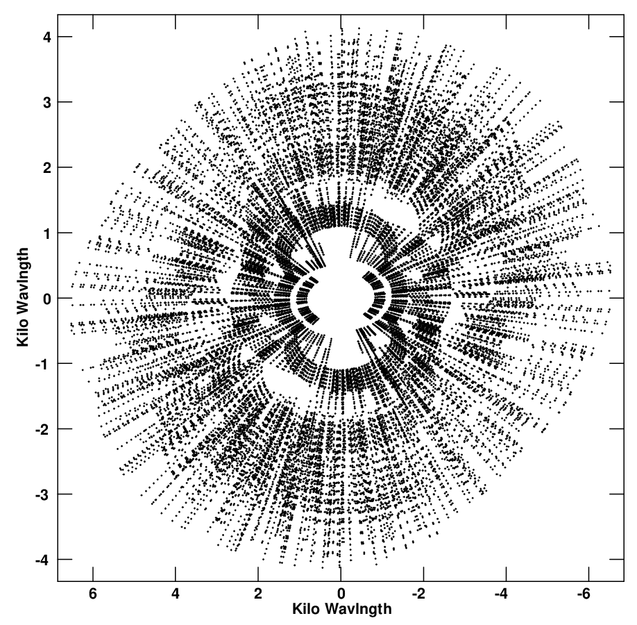
The sub-fields were each observed several times, typically for h at a time, until the desired noise levels were reached. The telescope dwell time per pointing was 30 s for the extended and 60 s for the core sub-fields. The dwell times were chosen so that in an observing run of typical length, each pointing was visited several times, serving to improve the uv-coverage. Fig. 2 shows the uv-coverage for a typical pointing in a final raster map. Owing to flagging of the data, for example due to poor weather conditions during observing, the noise was sometimes found to be higher than desired over small areas of the final map; these areas were targeted with additional, small rasters or with individual pointings to ensure more uniform coverage over the field.
5 Mapping
Raw data files from individual observing runs had various checks and calibrations applied using in-house, data-reduction software, reduce. A fuller explanation of the steps carried out in reduce, including the weighting of data depending on the weather conditions, can be found in AMI Consortium: Davies et al. (2009). The data were then output as multisource uv-fits files, which were, in turn, combined into a single multisource uv-fits file per field, again using in-house software.
Depending on the precise nature of the flagging applied, it is possible that data belonging to individual telescope pointings are constituted from different frequency channels in slightly varying proportions. As a consequence, when the data were combined into a single uv-fits file, the data weights were adjusted, on a pointing by pointing basis, so that the continuum maps would always have the same centre frequency: 15.7 GHz. This causes a small loss of sensitivity.
The uv-fits data were exported into the aips11 1 astronomical image processing system – www.aips.nrao.edu/ package and individual, continuum maps created for each telescope pointing using the imagr task. Each component map is 512 by 512 pixels, where the pixels are arcsec2 in size. Natural weighting was used to maximise signal-to-noise.
Each component map was cleaned using an elliptical Gaussian fitted to the central region of the dirty beam as the restoring beam. As a result, the restoring beam for each component map is slightly different – the implications of this for source extraction are discussed in Section 6.3. cleaning was stopped after the first negative clean component was reached, as real negative features are not expected to be present in the 10C maps. Negative clean components are in some cases necessary to best recover the true sky brightness distribution. However, we have chosen to adopt a conservative approach in order to avoid the so-called ‘clean bias’ (aips cookbook; www.aoc.nrao.edu/aips/cook.html), where real source flux is underestimated as a result of attributing clean components to noise fluctuations. The noise on each component map was then estimated using the imean task, which fits a Gaussian, centred on zero, to the distribution of pixel values.
Following a method similar to that of Waldram et al. (2003), the component maps were combined to form a single ‘raster’ map for each field, using the flatn task. Only data above the 0.1 power-point of the primary beam from each component map were used. The mapping was also attempted using a cut-off of 0.3, since the uncertainties in the primary beam increase with distance from its centre. However, this was found to produce significant discontinuities in the map, which in turn caused spurious source detections (see Section 8). Using a cut-off of 0.1 is found to make negligible difference to the source flux-densities and to the map noise and avoids the problem of sharp discontinuities in the map. For any point on the final raster map, data from between one and seven component maps contribute.
The map value at any point on the raster map is derived from the individual map, , primary beam, , and noise, , values of the relevant overlapping constituent maps, at that point. The maps are added, correcting for the primary beam, , and weighted according to the noise, , such that
A noise map, which provides an estimate of the noise at the same point on the raster map () is also computed, such that
Pixel values on both sky and noise maps are in Janskys per beam. The noise maps are found to provide an accurate representation of the noise. In particular, they are found to provide a better estimate of the true thermal noise close to sources, than would be found by considering the pixel values in the vicinity of sources on the real maps. Noise estimates computed using the latter method tend to be biased high.
Given the 4.0-arcmin spacing of the pointing centres and the 0.1 cutoff of the primary beam, if the noise level, , was the same on each component map then the noise in the main area of the raster map would vary between and . Fig. 3 is a small section of the noise map for one of the survey fields and shows the structure of the noise. There is necessarily a sharp increase in the noise at the edges of the map, as seen in Fig. 1.

6 Source extraction
Sources are detected in each survey field through analysis of the relevant raster map. For the 9C survey, candidate sources were followed up with pointed observations to allow identification of genuine sources. Observational time constraints meant that it was not possible to follow up each 10C source with a dedicated pointed observation. However, the 10C-survey noise maps provide much better estimates of the noise variation across the survey maps than were available as part of the 9C survey. Therefore, the noise maps were used to assess the reliability of each detection. Nevertheless, as described in Paper II, pointed observations were carried out towards of the brightest sources detected as part of the survey, providing a vital check of the raster maps’ flux-density scale.
In this section the steps in building a source catalogue are described. The methods employed are able to deal with noise levels and synthesised beams which vary across the maps. The source extraction is carried out using a combination of in-house software and aips. At the end of each subsection the parameters entered into the catalogue, at each of these steps, are provided. Source positions are quoted using equatorial coordinates (J2000).
6.1 Source identification and peak measurement
Source finding is carried out for each survey field making use of the noise map, which allows sources to be identified on the basis of their signal-to-noise ratios (SNRs). If one wishes to search for sources above , where is the value of the noise map at the pixel position and is a constant usually chosen to be 5.0, an initial search for pixels greater than is conducted. The value of 0.6 was found to be sufficiently low so as to identify all peaks that have values greater than after pixel interpolation. Pixels selected must have values greater than or equal to the surrounding eight pixels. Pixels at the map boundary are not considered as potential sources.
Since the synthesised beam is fully sampled ( 6 pixels per FWHM of the beam), for each candidate source a peak value, corresponding to a position interpolated between the grid points, is calculated. This is done by calculating the local map values on a successively finer grid (up to 128 times finer), by repeated convolution with a Gaussian-graded sinc function of the form
where has units of pixels (Rees, 1990). Interpolated peak values that are greater than or equal to are stored.
At this stage, the entries in the catalogue are (the interpolated peak flux density), and and (the interpolated peak position). The errors, , on the source peak-flux-densities are also provided. They are assumed to consist of a 5 per cent calibration error added in quadrature with the thermal noise estimate, because these are uncorrelated. Thus, the total error is . The source names contained in the catalogue are constructed from their respective coordinates.
6.2 Identifying overlapping/complex sources
Following a method similar to that of Waldram & Riley (1993), in-house software is used to identify overlapping sources. The integration area of a source is taken to consist of contiguous pixels down to a lowest contour level of 2.5. We begin by measuring the integration area of the source with the lowest value of . The source is classified as ‘single’ if its integration area contains no other peaks. Where more than one peak lies within the integration area, they are all classified as ‘overlapping’ and the name of the brightest peak, as well as the number of peaks, contained within the area are inserted in the ‘group’ column.
The above procedure is repeated for each of the sources that remain unclassified, in order of increasing . Considering the sources in this order avoids sources being classified as single when they actually lie within the contour of another source.
Sources can be separated by several synthesised beam widths, yet still share the same integration area because of the presence of faint extended emission linking them. Overlapping sources are therefore a good indicator of complex structure as well as point sources close together on the sky.
6.3 Gaussian-fitting
Next, the aips task, jmfit is used to fit a 2D elliptical Gaussian, by an iterative least-squares process, to each source. Angular sizes and integrated flux densities can be estimated from these Gaussian fits. For each source, the fitted Gaussian is compared to the point-source response. This enables the morphology of resolved sources to be characterised. This also provides a check for ‘over-narrow’ sources, which appear significantly smaller than the point-source response and are likely to be spurious. Such ‘sources’ can be caused by discontinuities in the map, for instance at the boundary of a constituent map. According to Condon (1997) they can also occur at the positions of noise bumps and between the peaks of overlapping or complex sources.
The comparison is complicated by the fact that the restoring beam is slightly different for each component map, as explained in Section 5. As most points on the raster map result from a combination of several constituent maps, the point-source response varies across the raster and cannot, in general, be characterised by a single 2-D elliptical Gaussian. In principle, this problem could be avoided by regrading the constituent maps with a single beam, having dimensions that encompass all the individual restoring beams. However, since in practice the beam areas vary significantly – by up to a factor of 2.24 for the most extreme field – this approach has not been adopted, as this would lead to a substantial loss of resolution. Rather, the point-source response belonging to the pointing with the highest weight at the position of the source is used in the comparison, as this proves to be a good approximation for the great majority of sources.
Due to the large number of sources detected in the 10C survey, the Gaussian-fitting has been automated. Six parameters are fitted for each single source: the peak value, peak RA and Dec., major axis, minor axis and position angle of the major axis. The fitting area consists of pixels inside a square centred on the source (peak) with a half-width of six pixels. Given the pixel size, this is sufficiently large to encompass point sources (for point sources at low SNR the 2.5- integration area is not sufficiently large). An exception is made if part of the integration area lies outside the box, in which case the size of the box is increased such that it encompasses the integration area, allowing correct fitting of extended sources. The fitted parameters are initialised as , , , , and (, and are the parameters of the restoring beam belonging to the pointing with the highest weight at the position of the source). A maximum number of 25 iterations is allowed to reach convergence. Even at low SNR, in real maps very few sources did not converge within this number of iterations. Those sources that failed to converge were found to lie on the sidelobes of bright sources and were often overlapping – they were excluded from the catalogue.
For overlapping sources of components, Gaussians are fitted simultaneously. The peak value, peak position, major axis, minor axis and position angle of the major axis of each component are allowed to vary. The fitting area consists of pixels within a box encompassing squares with half-widths of six pixels, one centred on each source (peak). Again, an exception is made if part of the integration area lies outside the box, in which case the size of the box is increased such that it encompasses the integration area. The values of , , , , and for each source are used to initialise the fit. A maximum number of 25 iterations is allowed to reach convergence.
Providing that the Gaussian-fitting achieves convergence, an integrated flux density, , is obtained. This is given by the peak height of the fitted Gaussian multiplied by the ratio of the area of the fitted Gaussian to that of the point-source response. For complex sources that are many times the size of the synthesised beam, a more accurate integrated flux density can be obtained simply by summing pixel values from the peak down to some SNR, normalising with respect to the beam. However, this method has not been implemented here, since there are no believable sources in the 10C survey for which the Gaussian-fitting does not converge. The Gaussian-fitting also provides useful additional information.
In addition, and , the fitted peak position is recorded. Following the method of Condon (1997), who has derived approximate and semi-empirical expressions for Gaussian-fitting errors in images with correlated noise, jmfit also provides an estimate of the error, , on , due to the thermal noise. The thermal noise, , is used by the task in estimating . Following Section 6.1, the total error on is taken as .
An estimate of the source size is obtained by deconvolving the point-source response from the fitted Gaussian (both represented by 2-D elliptical Gaussians). The sky brightness distribution is represented by the resulting 2-D elliptical Gaussian, the major and minor axes, and , and position angle, , of which are measured. For a point source in the limit of an infinite SNR this Gaussian will converge to a delta function. However, in the presence of noise the major axis will tend to be biased high (have a value greater than 0) and the minor axis low. In practice, axes for which the fitted value is negative are set to zero, as negative physical source sizes are not plausible. Table 2 summarises the interpretation of the major and minor axes, after deconvolution.
| Interpretation | ||
|---|---|---|
| +ve | +ve | Fitted Gaussian larger than point- |
| source response in all dimensions. | ||
| +ve | 0 | Fitted Gaussian larger than point- |
| source response in some dimension. | ||
| 0 | 0 | Fitted Gaussian equal to or smaller than |
| point-source response in all dimensions. |
The results of the deconvolution can be used to classify each source as point-like or extended. The classification criteria are justified fully in Section 7. Briefly, the source is classed as extended if is greater than or equal to some critical value, , given by Equation 7.
The catalogue entries for the Gaussian-fitting are, therefore, , , , , , , and . A flag, , is also included to denote one of two source types: point-like (P) or extended (E). As an additional check, for each source, the integrated flux density is normalised using the weighted sum of the areas of the point-source responses which contribute at the position of the source. If the resultant integrated flux density lies outside the range to then a ‘*’ is inserted in the ‘flag’ column. This indicates that the results obtained from the Gaussian-fitting must be treated with caution, since the error from the approximation of the point-source response is significant. In practice, this has been found to be the case for less than 1 per cent of sources above 5 detected in all survey fields.
6.4 Example catalogue
A contour plot of a small section of one of the survey fields, chosen since it provides a particularly interesting example, is shown in Fig. 4. A subset of the catalogue entries for the sources detected in this region are provided in Table 3. Table 4 lists the parameters which appear in the final source catalogues.

| Source | Group | (mJy) | (mJy) | () | () | () | (∘) | |||||
|---|---|---|---|---|---|---|---|---|---|---|---|---|
| 10CJ002209+312803 | 48.9 | 9.0 | P | |||||||||
| 10CJ002212+312317 | 27.5 | 8.6 | P | |||||||||
| 10CJ002223+312509 | 10CJ002224+312409(3) | 25.0 | 5.3 | P | ||||||||
| 10CJ002224+312409 | 10CJ002224+312409(3) | 25.0 | 9.1 | P | ||||||||
| 10CJ002227+312520 | 10CJ002224+312409(3) | 36.5 | 4.3 | P | ||||||||
| 10CJ002238+312622 | 31.0 | 7.1 | P | |||||||||
| 10CJ002246+313113 | 25.0 | 42.9 | 9.0 | 145.3 | E | |||||||
| Source | 10C source designation J2000 (6.1) |
|---|---|
| Group | 10C group designation J2000 (6.2) |
| RA (peak), in h, min, s (J2000) (6.1) | |
| Dec. (peak), in °, ′, ″ (J2000) (6.1) | |
| Peak flux density, in mJy (6.1) | |
| Error on peak flux density, in mJy (6.1) | |
| RA (fitted peak), in h, min, s (6.3) | |
| Dec. (fitted peak), in °, ′, ″(6.3) | |
| Integrated flux density, in mJy (6.3) | |
| Error on integrated flux density, in mJy (6.3) | |
| Critical component size, in ″(6.3) | |
| Major axis after deconvolution, in ″(6.3) | |
| Minor axis after deconvolution, in ″(6.3) | |
| Position angle after deconvolution, in °, | |
| measured from North through East (6.3) | |
| Source type (P = point-like, E = extended) (6.3) | |
| Flag | A star indicates that the approximation error for |
| the point-source response is significant (6.3) |
7 Classifying sources as point-like or extended
As noted in Section 6.3, criteria for classifying sources as point-like or extended have been developed. One approach would be to use the residuals from 3-parameter fits, where only the peak brightness, and peak RA and Dec. are allowed to vary, to identify extended sources; for extended sources the fit is expected to be poor. However, even for point sources the quality of the fit will vary with SNR and quantifying this dependence is difficult. An empirical approach might be possible. However, a method, based on theory, which makes use of the angular size after deconvolution has been found to provide a straightforward test applicable to a wide range of SNRs.
Maps containing point sources and noise were simulated in order to investigate the distribution of that would be expected for point sources as a function of SNR. Simulated visibilities were generated for point sources using uv-coverage from real observations of a survey field. After simulating the sources and noise in the uv-plane, the resultant multisource uv-fits file was mapped as described in Section 5 and source extraction was carried out as in Section 6.
Point sources were simulated in the uv-plane using a real multisource uv-fits file as a template. The visibility associated with the pointing, , was set to
where is the total number of sources, is the primary-beam-corrected flux density of the source, is a phase factor given by
| (6) |
and are the uv-coordinates of , and and are the RA and Dec. separations between the source and pointing centre respectively.
A source was only added to any individual pointing if it fell within 15 arcmin of the pointing centre. Beyond this distance its contribution was negligible owing to the fall-off in the primary beam. Gaussian noise was also simulated, such that the noise on each of the component maps was identical, by adding random numbers drawn from a Gaussian distribution to the real and imaginary parts of each visibility.
We note that point sources can alternatively be inserted into real raster maps by adding to real multisource uv data. Such simulations were carried out in order to assess the completeness of the 10C survey (see Paper II).
Our source extraction techniques were applied to a map of 3.2 deg2 containing 780, 100-mJy, simulated point sources – one at each pointing centre. The rms noise on each component map was simulated to be 10 mJy per beam. Once the component maps had been added together, as described in Section 5, the resulting rms noise varied between 8.6 and 9 mJy per beam over the central area of the raster map. For illustration, a section of this map is shown in Fig. 5.

Fig. 6 shows the distribution of for the simulated point sources with SNRs of approximately 10. It can be seen that it is very rare for a point source to have 40 arcsec at this SNR. However, as the SNR decreases, the distribution was found by doing runs with different source flux densities to move further away from zero and become wider and, as a result, 40 arcsec would not be a suitable dividing line between point and extended sources at all SNRs.

The minimum component size, , that can be measured is proportional to the FWHM of the synthesised beam and inversely proportional to the square root of the SNR (Fomalont, 2006). Fig. 7 shows the median value of versus , where , for artifical point sources with SNRs ranging between 7 and 1000. It can be seen that the expected relation is obtained for . The relation starts breaking down at higher SNRs. This is probably due to the limited level of accuracy with which we are able to simulate data, produce maps and recover source parameters. For instance, the maps have a finite pixel resolution which will affect the accuracy with which angular sizes can be measured. In any case, calibration errors are the dominant source of error for .

These results indicate that ought to be a useful indicator of source extension. Fig. 8 shows the distribution of for the point sources with SNRs of approximately 10. Fewer than 1.2 per cent of sources have . In addition, the distributions of for sources with SNRs ranging between 7 and 100 were investigated. In each case, less than 1.5 per cent of sources were found to have . As noted above, at high SNRs, calibration errors will become the main source of uncertainty. As a result, sources with arcsec are never considered to be extended, no matter how high the SNR. This value corresponds approximately to the critical value at a SNR of 20, above which calibration errors begin to dominate. On the basis of our findings, a source is classified as extended if , where

Clearly, there is no sharp dividing line between point and extended sources, and no single method for making the distinction. However, the above procedure for estimating source sizes is simple and robust, and is able to deal with sources with a wide range of SNRs. The expected percentage of point sources which are misclassified as extended in this scheme is per cent. The minimum angular size that can be measured is estimated as a function of both the telescope resolution and the SNR. The median value of for each survey field varies between 32.5 and 42.6 arcsec.; it is generally lower for a field lying at a higher declination. Fig. 9 shows how varies with SNR for arcsec.

The method for distinguishing between point and extended sources can be used to establish how best to measure the total flux density of a source. Clearly, should be used to estimate the total flux density of an extended source. Both and can be used to describe a point source. However, at low SNR, the results obtained using will be significantly less accurate given the fact that the source is not assumed to be point-like when measuring . In summary, should be used to describe all sources except those that are classified as extended, for which should be used.
8 Application of source extraction techniques to real data


To illustrate the source extraction procedures outlined above they were applied to one of the survey fields, covering an area of about 2.5 ; the results are presented here. The noise levels in the core and extended field areas are typically 50 and respectively. In total, 158 sources were detected above , of which 10 are classed as overlapping.
The Gaussian-fitting converged successfully for all sources within 25 iterations. Fig. 10 shows how compares with for all sources, 10 of which are classified as extended.
No over-narrow sources were detected. However, when using a primary beam cut-off of 0.3 to map the data several sources were found to have integrated flux-densities significantly smaller than their peak flux-densities. This is indicative of a spurious source. These detections were found to be separated from other sources (spurious or real) by a distance much smaller than a synthesised beam FWHM. This is implausible and resulted from the edge of a component map passing through a genuine source – this resulted in a sharp discontinuity in pixel values (Fig. 11).
9 Conclusions
In order to investigate the high-frequency-radio sky we have observed 10 survey fields, covering deg2 to an rms noise level of , using the AMI LA at 16 GHz. In an accompanying paper, AMI Consortium: Davies et al. (2010), we present the first results from the survey, including the deep 15.7-GHz source count. Here, we have concentrated on developing techniques for producing and analysing the survey raster maps. In particular, we have:
- (1)
developed systematic, automated methods for identifying and characterising sources in maps with varying noise levels and sythesised beams.
- (2)
proposed a straightforward and robust method for distinguishing between point and extended sources over a wide range of SNRs. Our method has been tested using maps including simulated sources and noise, and has been shown to be successful in identifying extended emission.
- (3)
applied our techniques to real sky maps and demonstrated that our automated techniques are useful for identifying and chracterising complex structure (see, for example, Fig. 4).
Acknowledgments
We are grateful to the staff of the Mullard Radio Astronomy Observatory for the maintenance and operation of the AMI. We thank the referee, Elaine Sadler, for helpful comments. We are also grateful to the University of Cambridge and PPARC/STFC for funding and supporting the AMI. MLD, TMOF, MO, CRG, TWS and MPS are grateful for support from PPARC/STFC studentships.
References
- Browne et al. (1998) Browne I. W. A., Wilkinson P. N., Patnaik A. R., Wrobel J. M., 1998, MNRAS, 293, 257
- Cornwell (1988) Cornwell T. J., 1988, A&A, 202, 316
- Condon (1997) Condon J. J., 1997, PASP, 109, 166
- AMI Consortium: Davies et al. (2009) AMI Consortium: Davies M. L. et al., 2009, MNRAS, 400, 984
- AMI Consortium: Davies et al. (2010) AMI Consortium: Davies M. L et al., 2010, in preparation
- Fomalont (2006) Fomalont E., 2006, Lecture at Tenth Summer Synthesis Imaging Workshop, University of New Mexico, USA
- Patnaik et al. (1992) Patnaik A. R., Browne I. W. A., Wilkinson P. N., Wrobel J. M., 1992, MNRAS, 254, 655
- Rees (1990) Rees N., 1990, MNRAS, 244, 233
- Rudy et al. (1987) Rudy D. J., Muhleman D. O., Berge G. L., Jakosky B. M., Christensen P. R., 1987, Icarus, 71, 159
- Sault et al. (1996) Sault R. J., Staveley-Smith L., Brouw W. N., 1996, A&AS, 120, 375
- Waldram & Riley (1993) Waldram E. M., Riley J. M., 1993, MNRAS, 265, 853
- Waldram et al. (2003) Waldram E. M., Pooley G. G., Grainge K. J. B., Jones M. E., Saunders R. D. E., Scott P. F., Taylor A. C., 2003, MNRAS, 342, 915
- Waldram et al. (2010) Waldram E. M., Pooley G. G., Davies M. L., Grainge K. J. B., Scott P. F., 2010, 404, 1005
- Watson et al. (2003) Watson R.A. et al., 2003, MNRAS, 341, 1057
- Wilkinson et al. (1998) Wilkinson P. N., Browne I. W. A., Patnaik A. R., Wrobel J. M., Sorathia B, 1998, MNRAS,300, 790
- AMI Consortium: Zwart et al. (2008) AMI Consortium: Zwart J. T. L. et al., 2008, MNRAS, 391, 1545